A Study of the Afterglows of Four GRBs: Constraining the Explosion and Fireball Model

Abstract

We employ a fireball model of the gamma-ray burst explosion to constrain intrinsic and environmental parameters of four events with good broadband afterglow data; GRB 970508, GRB 980329, GRB 980703, and GRB 000926. Using the standard assumptions of constant circumburst density and no evolution of the fraction of the explosion energy in the post-shock magnetic field, we investigate the uniformity of the derived explosion and shock physics parameters among these events. We find a variety of parameters: densities that range from those of the ISM to diffuse clouds, energies comparable to the total GRB $\gamma$-ray energy, collimations from near-isotropy to 0.04 radians, substantial electron energy fractions of 10-30% with energy distribution indices of 2.1-2.9 and magnetic energy fractions from 0.2-25%. We also investigate the level to which the data constrain the standard model assumptions, such as the magnetic field evolution, and the allowed density profiles of the medium. Fits generally improve slightly with an increasing magnetic energy fraction $\epsilon_{B}$. Good fits can be produced with magnetic energy accumulating or decaying with the shock strength over the afterglow as $\epsilon_{B}\propto\gamma^{x}$; $-2\leq x\leq+1$ . The data are not very sensitive to increasing density profiles, allowing good fits even with density $\propto r^{10}$. Some parameter values change by up to an order of magnitude under such altered assumptions; the parameters of even good fits cannot be taken at face value. The data are sensitive to decreasing densities; $r^{-2}$ profiles may produce reasonable fits, but steeper profiles, even $r^{-2.5}$, will not fit the data.

1 Introduction

Afterglow emission, spanning from radio to X-ray, and observable from minutes to weeks after the event, appears to be a ubiquitous feature of long-duration gamma-ray burst explosions. Afterglows result from radiation emitted by electrons accelerated in a relativistic shock produced by the explosion of a progenitor (e.g., Paczyński & Rhoads, 1993; Katz, 1994). As the shock propagates outward into the surrounding medium, the resulting broadband synchrotron radiation evolves in a manner dependent on a number of fundamental characteristics of the explosion, as well as on the details of the shock evolution and the density profile of the medium it expands into (for a review of the theory, see Mészáros, 2002).

The physics of relativistic shocks, the mechanism of collisionless shock acceleration, and the means by which magnetic fields can be amplified to levels needed to produce the observed synchrotron emission are poorly understood. Basic understanding of these elements will eventually result from improved magnetohydrodynamic simulations, which may ultimately prescribe such factors as the appropriate electron energy distribution, what fraction of shock energy goes into magnetic field, and how this evolves with the shock expansion. Additional uncertainties arise from the fact that the outflow geometry, and the structure of the circumburst medium are unobservable, and could potentially be complex.

In spite of the lack of detailed understanding, the basic features of the GRB afterglow can be described by relatively simple theoretical models for the outflow and shock (e.g. with relativistic flow as in Blandford & McKee, 1976). Simple assumptions about the shock microphysics and geometry appear to fit the basic features of the afterglow in a number of cases (e.g., Wijers & Galama, 1999; Chevalier & Li, 2000; Harrison et al., 2001; Panaitescu & Kumar, 2001b, a, 2002). In addition, many events appear consistent with the expansion of the shock into a medium with either a constant or a simple $r^{-2}$ powerlaw in density.

Ideally, high-quality broadband afterglow observations, interpreted in the context of basic theoretical models, could be used to constrain the explosion parameters, geometry, and the structure of the surrounding medium. In addition, if the data are of sufficiently high quality, it should be possible to test the validity of the basic model assumptions; or at least the range over which they may be varied and still describe the data. Given a relatively large number of model parameters, however, only a few data sets are of sufficient quality to provide interesting constraints.

In this paper, we examine four high-quality broadband afterglow data sets, fitting them to a basic afterglow model. We investigate the similarity of the derived explosion, shock, and environmental parameters. In addition, we investigate selected model assumptions and the range over which they can be varied. In particular, we consider whether the fraction of energy in the post-shock magnetic field can evolve as some power of the bulk Lorentz factor, and the range of possible matter density gradients. Finally, we consider which future observations provide the most promise for better constraining both the model and its physical parameters.

2 The Afterglow Framework

We adopt a standard fireball scenario for the GRB afterglow, where a relativistic shock with Lorentz factor $\gamma$ expands into the circumburst medium (CBM). Blandford & McKee (1976) describes the flow. The shock may be spherical or initially confined to a cone (i.e., be jet-like). The afterglow flux arises from the radiation (synchrotron and possibly also inverse Compton) emitted by relativistic electrons accelerated in the shock. To describe its evolution we model the shock dynamics, adopting assumptions for the density profile of the CBM, the shock geometry, and the shock microphysics including the distribution of electron energies, as described below. We also account for the effects of the medium through which the radiation passes en route to the observer.

2.1 The Basic Afterglow Model

For the dynamics, we make simple assumptions about the event’s geometry and environment. We consider a constant circumburst matter density $n$, the “ISM-like” case, as well as the possibility the CBM could be dominated by a wind outflow from the progenitor. As a constant mass-loss rate and wind speed gives an $r^{-2}$ profile, we consider this the “Wind-like” case. Into either CBM form we allow for isotropy or a simple collimation of the ejecta, a top-hat distribution in solid angle with half-opening angle $\theta$. The shock behaves as though isotropic until it slows down sufficiently to expand in its rest frame (Rhoads, 1999; Sari, Piran & Halpern, 1999). We calculate the time $t_{jet}$ at which collimation is evident as $\theta$ = 1/$\gamma$ ($\gamma$ the shock Lorentz factor; this assumes the observer is nearly along the line of sight). We calculate the expected radiative losses, which can modify the shock dynamics (Sari, 1997), in the manner detailed further below.

For the microphysics governing the emission it is standard to assume several things. First, that the shock imparts a constant fraction of its energy ($\epsilon_{e}$) to the swept-up electrons, and a constant fraction ($\epsilon_{B}$) goes into amplifying magnetic fields. These fractions are capped at 100%, where all the shock’s energy would be in one of these. A reasonable limit could have been the ejecta-$\epsilon_{e}$-$\epsilon_{B}$ equipartition value of 33%, but the model’s calculations are not perfectly known. The equations used have some uncertainties; we allow each of $\epsilon_{e}$ and $\epsilon_{B}$ to vary up to the limit of taking all the shock energy. It is also assumed that the electrons are accelerated into a simple powerlaw distribution of energies above a minimum value (P($\gamma_{e}$)$\propto\gamma_{e}^{-p}$, $\gamma_{e}>\gamma_{m}$), with a constant index $p$.

These are our basic assumptions for the fireball model. They will be tested in further sections.

2.2 The Emission calculation

Given this electron spectrum, we get a broken powerlaw radiation spectrum, with three break frequencies that evolve in a manner that depends upon the dynamics (Sari, Piran & Narayan, 1998): the injection break $\nu_{m}$ for the minimal energy of the radiating electrons, the cooling break $\nu_{c}$ corresponding to energies at which radiative losses over the shock’s lifetime are significant and the self-absorption break $\nu_{a}$ where the spectrum becomes optically thick at low frequencies. If the minimum energy electrons emit at a peak frequency above the self-absorbed regime, the spectrum below $\nu_{a}$ is $\propto\nu^{2}$, ressembling a blackbody with effective temperature corresponding to that minimum energy; if electrons are emitting within the optically thick regime, the effective temperature is a function of frequency and the spectrum is $\propto\nu^{5/2}$ (Rybicki & Lightman, 1979). We use a smooth shape with factors of (1 + $(\nu/\nu_{break})^{\beta_{1}-\beta_{2}}$)^-1 ($\beta_{1,2}$ are the indices before and after the break) for $\nu_{m}$ and $\nu_{c}$, and for $\nu_{a}$ we use the physically motivated prescription of Granot, Piran & Sari (1999a).

For the model with basic assumptions we employ the previously published fireball model calculations for the spectral breaks. The isotropic case is taken from Sari, Piran & Narayan (1998)’s relativistic near-adiabatic case, with normalizations from Granot & Sari (2002) (their canonical order, Table 2) for a Wind-like CBM, and from Sari, Piran & Narayan (1998); Granot, Piran & Sari (1999a, b) for an ISM-like CBM. These normalizations account for the post-shock spatial distribution of electrons and emission from equal arrival-time surfaces. The resulting equations are:

$$\begin{array}[]{lccc}F_{\nu}^{max}&=&1.6\,(z+1)\,D_{28}^{-2}\,\epsilon_{B,-2}^{0.5}\,E_{52}\,n^{0.5}&{\rm mJy}\\ \nu_{a}&=&4.2\times 10^{8}\,(z+1)^{-1}\,f_{I}(p)\,\bar{\epsilon}_{e}^{\,-1}\,\epsilon_{B,-2}^{0.2}\,E_{52}^{0.2}\,n^{0.6}&{\rm Hz}\\ \nu_{m}&=&3.3\times 10^{14}\,(z+1)^{0.5}\,\epsilon_{B,-2}^{0.5}\,\bar{\epsilon}_{e}^{2}\,E_{52}^{0.5}\,t_{d}^{-1.5}&{\rm Hz}\\ \nu_{c}&=&6.3\times 10^{15}\,(z+1)^{-0.5}\,\epsilon_{B,-2}^{-1.5}\,E_{52}^{-0.5}\,n^{-1}\,t_{d}^{-0.5}&{\rm Hz}\\ \end{array}$$ (1)

For the ISM-like CBM, where $f_{I}(p)=(\,(p+2)(p-1)/(3p+2)\,)^{0.6}$ and $\bar{\epsilon}_{e}=\epsilon_{e}(p-2)/(p-1)$. For the Wind-like CBM:

$$\begin{array}[]{lccc}F_{\nu}^{max}&=&7.7\,(p+0.12)\,(z+1)^{1.5}\,D_{28}^{-2}\,\epsilon_{B,-2}^{0.5}\,E_{52}\,A_{*}\,t_{d}^{-0.5}&{\rm mJy}\\ \nu_{a}&=&3.3\times 10^{9}\,(z+1)^{-0.4}\,f_{W}(p)\,\bar{\epsilon}_{e}^{\,-1}\,\epsilon_{B,-2}^{0.2}\,E_{52}^{-0.4}\,A_{*}^{1.2}\,t_{d}^{-0.6}&{\rm Hz}\\ \nu_{m}&=&4.0\times 10^{14}\,(p-0.69)\,(z+1)^{0.5}\,\epsilon_{B,-2}^{0.5}\,\bar{\epsilon}_{e}^{2}\,E_{52}^{0.5}\,t_{d}^{-1.5}&{\rm Hz}\\ \nu_{c}&=&4.4\times 10^{13}\,(3.45-p)e^{0.45p}\,(z+1)^{-1.5}\,\epsilon_{B,-2}^{-1.5}\,E_{52}^{0.5}\,A_{*}^{-2}\,t_{d}^{0.5}&{\rm Hz}\\ \end{array}$$ (2)

where $f_{W}(p)=(\,(p-1)/(3p+2)\,)^{0.6}$. The units are: $D_{28}$ = luminosity distance in 10²⁸ cm, $\epsilon_{B,-2}$ = $\epsilon_{B}$ in %, $n$ = density in cm^-3, $A_{*}$ = density scaling for the Wind-like profile so that $\rho=5\times 10^{11}\,A_{*}\,r^{-2}$ g cm^-1 ($r$ in cm; a standard reference for a mass loss of 10${}^{-5}\;$M${}_{\odot}\;$yr^-1 at a wind speed of 1000 km s^-1), $E_{52}$ = isotropic-equivalent energy in units of 10⁵² ergs, $t_{d}$ = observed time post-burst in days. The electron energy partition $\epsilon_{e}$ is given as a fraction.

The post-$t_{jet}$ evolution with laterally expanding ejecta uses the time-dependences of Sari, Piran & Halpern (1999) (eqs. 2-5), and is connected to the pre-jet behaviour without smoothing (i.e., a sharp jet break).

Using the relativistic equations for the shock energy, $E=M\gamma^{2}$, we calculate the time at which $\gamma=1$ as the nonrelativistic transition, $t_{nr}$. This would be equivalent to using the Blandford & McKee (1976) approximation for the energy, $E=M\gamma^{2}\beta^{2}$, and defining the nonrelativistic transition condition as $\gamma\beta=1$. We again employ a sharp transition to the post-$t_{nr}$ behaviour.

We adjust this evolving synchrotron spectrum with self-consistent corrections to the cooling rate, based upon the parameters already enumerated. We calculate the effects of synchrotron photon upscatters (inverse Compton scatters, IC) off the shocked electrons as in Sari & Esin (2001). When IC dominates the cooling we adjust the cooling break $\nu_{c}$ (by $(1+Y)^{-2}\approx Y^{-2}$ when $Y>1$; $Y$ the IC to synchrotron luminosity ratio $\approx$ (max[$(\gamma_{c}/\gamma_{m})^{2-p}$,1]$\epsilon_{e}/\epsilon_{B}$)^1/2). The upscattered photons can produce a high-frequency secondary source of flux; for it we adopt the spectral breaks as in Sari & Esin (2001) and use our synchrotron spectral shape (a good approximation except for an ignored logarithmic correction between $\nu_{m}^{IC}$ and $\nu_{c}^{IC}$ and the slope for $\nu<\nu_{a}^{IC}$, where IC never dominates the data).

We also treat radiative corrections self-consistently, from the model parameters. Instantaneously, we treat the shock as adiabatic. The energy is calculated for each time from the solution of $dE/E$ (Cohen, Piran & Sari, 1998). It depends upon the ratio $\nu_{c}/\nu_{m}$ in slow cooling ($\nu_{c}>\nu_{m}$) as the losses quench out and we use the synchrotron-only rate of change in $\nu_{c}$, allowing a simple analytic solution for $E(t)$. As this is when $E(t)$ changes are becoming unimportant, the approximation has little effect. We scale the shock’s energy to the value at the change from fast- to slow-cooling regimes ($\nu_{c}=\nu_{m}$, fairly early).

This spectrum is modified on the way to the observer, and we must account for extinction, interstellar scintillation (ISS) and the host’s flux. ISS in the Galaxy distorts the flux at low (radio) frequencies; we estimate its fractional flux variations as outlined in Walker (1998) for point sources, using the map of scattering strengths by Taylor & Cordes (1993), and scalings for extended sources as explained in Narayan (1992). The growing angular size quenches the scintillations; we assume initial parameters in the model to get angular size as a function of time for the ISS model. These are not iterated, but used as an additional uncertainty in the model flux, added in quadrature to the data’s uncertainties when estimating $\chi^{2}$.

For extinction, we first deredden for Galactic effects using Schlegel, Finkbeiner & Davis (1998)’s method for estimating A_λ in the optical. As most GRBs are at high Galactic latitudes, this term is small. Then, as the extinction curves in high-$z$ galaxies are unknown, we use known local extinction curves redshifted to the host restframe to fit for host contributions. We use Weingartner & Draine (2001)’s Large Magellanic Cloud (LMC) in general, but for the GRB 980329 event we used the Small Magellanic Cloud Bar’s law due to evidence that the host’s extinction law is steep. We do not subtract host fluxes as the decay slope is sensitive to small differences in the host value; host fluxes are added to the model in the fit. In the optical and near-IR, when there is evidence for a host component, we fit a value for the particular band(s) involved. As submillimeter hosts have been detected in other bursts (Hanlon et al., 2000; Berger, Kulkarni & Frail, 2001; Berger et al., 2001; Frail et al., 2002; Berger et al., 2003), we allowed for this possibility (scaled to 350 GHz as $\nu^{3}$), but none was required for the four events under consideration and this component was not included in the best fits. Finally, we see in 2 datasets evidence for underlying flux in the radio. 980703 has sufficient data that a spectral index (-0.32, Berger, Kulkarni & Frail, 2001) was determined and we fit the radio host flux scaled to 1.43 GHz (where it is brightest). For 980329 we use a canonical spectral index of $\nu^{-0.8}$, again scaled to 1.43 GHz.

Two other groups have performed full analyses similar to ours, as described in Chevalier & Li (2000); Li & Chevalier (2001) and Panaitescu & Kumar (2001b, a, 2002). There are some differences in each group’s approach to the fireball model. Chevalier & Li develop an $r^{-2}$ CBM model, including analytic solutions to the hydrodynamics, but they do a numerical solution to get the full smooth spectral shape. They assume an extra break in the electron energy distribution but do not, however, account for energy losses, IC cooling or ISS effects. Panaitescu & Kumar numerically solve the dynamics (whereas we use analytic asymptotic forms), numerically calculate the spectrum from equal arrival-time surfaces (whereas we use equations adjusted to account for equal arrival-time surfaces and the electron distribution behind the shock, and a simple smoothing) and calculate IC scatters and energy losses directly from the model’s radiated spectrum (whereas we use the theoretically expected levels from the parameters). They use the simplest electron energy distribution when it provides a good solution but also allow for two (rather than one) indices in the injected spectrum if needed. They pre-account for host effects by subtracting fluxes and fixing extinction levels, instead of including these in the fits.

3 The Sample of Four GRBs

We selected four events with rich datasets (radio, optical-NIR and X-ray at a minimum) for which the fireball model with simple assumptions provides a good description of the lightcurves. These are GRB 970508, detected by the BeppoSAX GRBM instrument, with its X-ray afterglow found by the BeppoSAX WFC (Costa et al., 1997), GRB 980329, its afterglow detected in the X-rays by In ’t Zand et al. (1998), GRB 980703, detected by BATSE (Kippen et al., 1998) with its afterglow identified by the Rossi X-Ray Timing Explorer (Levine, Morgan & Muno, 1998) and GRB 000926, located by the IPN (Hurley et al., 2000; Hurley, 2000), with its afterglow first identified in the optical (Gorosabel et al., 2000; Dall et al., 2000).

We compiled and described the afterglow data for the 980329, 980703 and 000926 events in previous papers. The summaries presented here chiefly point the reader to the relevant papers. As we have not compiled the 970508 data elsewhere, we provide full details here.

GRB 970508 was the second burst with a detected afterglow, and it has a rich broadband dataset. We use the X-ray fluxes of Piro et al. (1998), converting to flux densities and frequency assuming $\nu^{-1.1}$ over their quoted band. For the optical/NIR, we use BVI data from Sokolov et al. (1998) and Zharikov, Sokolov & Baryshev (1998), R from the table compiled in Garcia et al. (1998), and K_s from Chary et al. (1998). We converted magnitudes to flux densities with the information in Tokunaga (2000) for K_s and Bessell (1979) for BVRI. We included the 12-$\mu$m mid-IR measurement by Hanlon et al. (1999). We used Bremer et al. (1998) in the submillimeter (86 & 232 GHz), and the 15 GHz data of Taylor et al. (1997) and the 1.43, 4.86 and 8.46 GHz dataset of Frail, Waxman & Kulkarni (2000) in the radio.

GRB 970508’s afterglow was unusual - a sudden brightening in (at least) the optical occurred at $\sim$ 1 day, followed by the usual powerlaw decays at $t\geq 2$ days, and the dataset shows an intrinsic “scatter” even at later times in at least the optical and radio. No simple model can account for the rise. Various possible explanations for a sudden rise in afterglow flux include a refreshed shock from slower material in the relativistic flow catching up to the slowing forward shock (Panaitescu, Mészáros & Rees, 1998; Sari & Mészáros, 2000; Kumar & Piran, 2000), a sudden jump in the encountered density (Wang & Loeb, 2000; Dai & Lu, 2002; Nakar, Piran & Granot, 2003), or even the “patchy shell” model where there are hot and cold spots in the shock and as the shell slows a hot spot may come into the observable area (Nakar, Piran & Granot, 2003). These models can provide a single rise that will not affect the emission substantially later. To avoid such complications we used only the data at $t\geq 2$ days, after the rise, for the modelling dataset.

The 980329 event has data in the X-ray, optical, submillimeter and radio regimes. Initial searches in the optical were unsuccessful, and Taylor et al. (1998) first identified the afterglow in the radio. Early epoch optical data where the afterglow dominates over host emission is therefore somewhat sparse. The excess $t<3$ days emission at 8.46 GHz is thought to be due to a reverse shock (Sari & Piran, 1999b) and therefore we excluded it from our analysis. Yost et al. (2002) gives full details concerning the dataset. No redshift has been determinable for this event (the only such case in our sample) due to faint host emission and a lack of prominent emission lines; we adopt z=2 here, roughly the middle of the potential redshift range.

The 980703 afterglow data includes radio, optical/NIR (with good frequency coverage: BVRIJHK) and X-ray. The utility of the opt-NIR data is limited to a few days postburst by a bright host (which is also visible in the late radio data). Frail et al. (2003) give the details.

The 000926 afterglow data includes radio data from 1.43 to 98 GHz, ground-based and HST optical and NIR observations and Chandra X-ray observations. The first 8.46 GHz point ($\approx$ 1.2 days postburst) was excluded from the analysis as abnormally high and possibly associated with reverse shock emission. We use all available BVRHK data and divide the X-ray into a soft and a hard band. This is further described in Harrison et al. (2001).

4 Fits to the Basic Model

970508 shows a “scatter” in its lightcurves in all frequency regimes and timescales. It is not clear how much of the scatter may be due to real physical effects (such as clumpiness in the circumburst medium), and how much could be attributed to cross-calibration uncertainties. While we performed our fits as in §2, the best fit, passing through the data, has $\chi^{2}$/DOF $\approx$ 2.5. (We do not attempt an analysis with increased error bars to reduce $\chi^{2}$ to the DOF, as this would require much larger uncertainties.) We have adopted this fit, a nearly-isotropic solution ($t_{jet}=183$ days) with an ISM-like CBM of somewhat low density (0.2 cm^-3) and $\epsilon_{e}$ and $\epsilon_{B}$ near equipartition, as our best solution.

Yost et al. (2002) fit 980329 as detailed in §2. Our best model is collimated, with a significant density (n $\sim$ 20 cm^-3) and host extinction. We found no need for a submillimeter host component, and that a radio host improves the fit with marginal significance. The best fit was not a unique solution; Yost et al. (2002) noted an isotropic, extremely radiative (all the shock’s energy in radiating electrons) solution fit as well. We reject that solution on the basis of its unphysical parameters.

Frail et al. (2003) gives results of 980703’s fits as in §2. The best fit is a collimated jet into a constant density CBM, its jet break hidden in the optical by the host’s dominance. It was not a unique solution; a collimated jet in an $r^{-2}$ CBM fit the data equally well. That fit required extreme parameters: 70% of the shock’s energy is imparted to the electrons and the energy during the afterglow is $\mathrel{\hbox{\hbox to0.0pt{\lower 2.36806pt\hbox{$\sim$}\hss}\kern 0.0pt\raise 1.72218pt\hbox{$<$}}}$ 1/10 that of the prompt $\gamma$-ray emission, requiring an extremely high $\gamma$-ray conversion efficiency. We reject the $r^{-2}$ fit.

The model we employ (§2) for the 000926 fits has changed since the work done in Harrison et al. (2001). Before, estimated host fluxes were subtracted instead of fitted for. As there was a galaxy “arc” nearby contaminating the ground-based data, the host components fitted for are merely the persistent underlying flux common to both ground- and space-based observations; the “arc” flux removal remains as before. Moreover, the model now employs radiative corrections to the energy, which were not yet incorporated in the previous analysis. We refit the dataset; the best fit from the improved model is in Table 1. It is still a high-IC ISM model with a substantial density, but the $\chi^{2}$ has increased. The previous fit had a nonnegligeable $\epsilon_{e}$ and no radiative corrections; with radiative corrections correlated with $\epsilon_{e}$, these are incompatible, $\epsilon_{e}$ drops and the fit worsens. In particular, while the X-ray still requires flux above the synchrotron’s level, the parameter changes cause the IC flux estimate to no longer match the data as well.

4.1 Comparisons of the Four Bursts

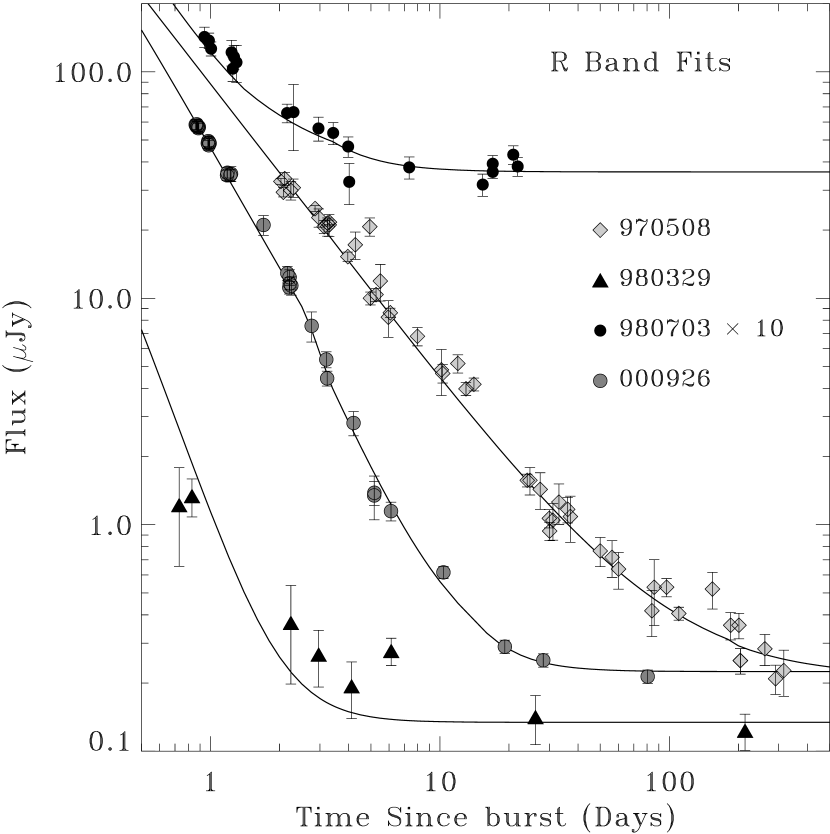
Figure 1: Subsets of the optical data from the best fits - the R band light curves for the four events. For data selection, see §3. The fits shown are to the full broadband datasets, with typically 100+ DOF, and are detailed in Table 1. The GRB 980329 optical data is not very constraining for the decay rate - a late optical detection (the early points were found on reanalysis) did not allow deep followup over the first week. The scatter in the GRB 970508 data cannot be explained in any simple model, and otherwise the fits are quite good.

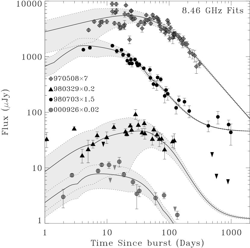
Figure 2: 8.46 GHz light curves of the 4 events, with the best fits (see Table 1). The light grey envelopes show the estimate of the model uncertainty due to interstellar scintillation, and data that is not statistically significant at the 2-$\sigma$ are presented as 2-$\sigma$ upper limits (downward triangles). As explained in §3 the data for GRB 980329 prior to day four likely contains an excess contribution from the reverse shock and was therefore not included in the fit. The 980329 radio host component only marginally improves the fit, due to a 1.43 GHz average excess, which may indicate a weak radio host flux. The fits are overall quite good, although ISS cannot fully account for the scatter in the 970508 dataset (there is, moreover, inexplicable scatter at other frequencies).

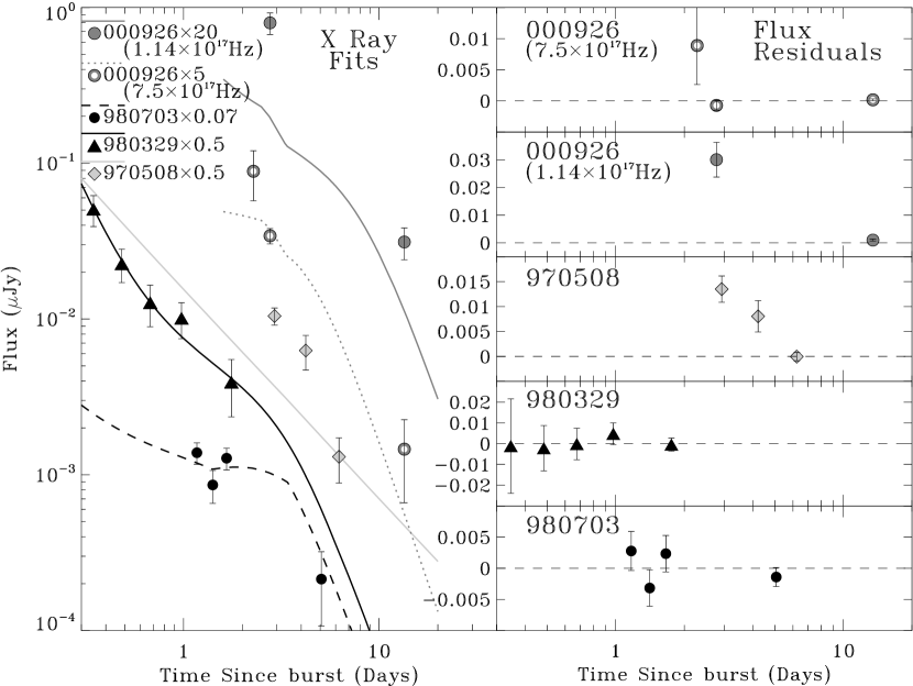
Figure 3: The X-ray data of the 4 events, with the best fits (see Table 1). To parse out which model goes with each dataset, the line style is indicated above the symbol labels, and linearly-scaled residuals are on the right. The GRB 000926 data is divided into a soft (solids) and a hard (open circles with dotted line) band. The broadband fit (with relative flux levels and decay rates) indicates an extra flux component in the X-ray, possibly Inverse Compton upscatters, but our estimate of this component does not completely fit the data. Better sampled X-ray lightcurves, such as those expected from Swift, may clarify deficiencies in the X-ray flux model. There is additionally a minor IC flux component in the GRB 980329 model, and IC dominates the early GRB 980703 X-ray model, providing the flat initial flux and slow decay to match the data.

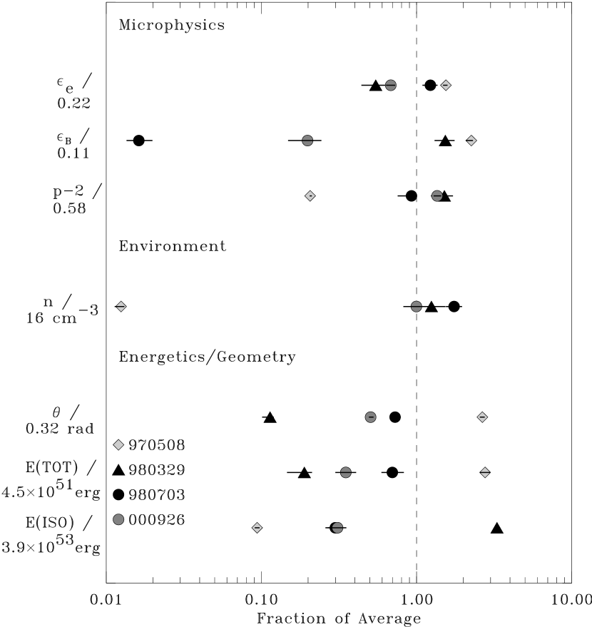
Figure 4: Parameters from the best fits with the simple model assumptions (see Table 1). They are divided into 3 categories: energy & geometry (kinetic energy, collimation half-opening angle $\theta$), environment (density) and microphysics (energy partitions: $\epsilon_{e}$ for electrons, $\epsilon_{B}$ for magnetic fields, and electron energy distribution index $p$). See §2 for further details concerning the fireball model’s parameters. They are presented relative to a nominal value as indicated; the error bars are statistical only, 68.3% intervals calculated via Monte Carlo bootstraps. The model uncertainties are larger, as seen in the Tables’ range of parameters that produce reasonable fits under various assumptions. The diversity in energy, geometry and environment is not unexpected for some variation in progenitor properties. Shock physics, however, is expected to depend only on shock strength. The variation of these parameters by orders of magnitude suggests that some effect is unaccounted for in the model.

Table 1 presents the best fits using the basic assumptions described in §2.1 (also see Figure 4). The table includes statistical 68.3% confidence intervals for the parameters, calculated from (non-Gaussian) distribution histograms generated by over 1000 Monte Carlo bootstraps. The results show a great deal of diversity in the values, similar to other efforts (e.g. Panaitescu & Kumar, 2001b). The fits can be seen in Figures 1, 2, 3.

Neither the variation in nor the values of the energy/geometry and environmental parameters is surprising. Variation is seen in the energies of the prompt GRB emission (Frail et al., 2001). Moreover, if GRBs are related to the deaths of massive stars (see the review by Mészáros, 2002, and references therein) then we would not expect such parameters to be identical due to variations in progenitor mass, angular momentum and environment.

The densities are comparable to the Milky Way’s ISM density at the low end, and to the density of diffuse clouds for the three $\sim$ 20 cm^-3, typical of other efforts with significant radio data (which constrains the synchrotron self-absorption) (e.g., Panaitescu & Kumar, 2001a). The values are not inconsistent with the core-collapse GRB progenitor hypothesis, despite the expectation of a stellar birth environment, and molecular cloud cores having $n\gg 10^{4}$ cm^-3. Diffuse clouds are also associated with star-forming regions, and such densities are found in the interclump medium that dominates molecular cloud volumes in the Galaxy (Chevalier, 1999, and its references). Moreover, massive stars modify their environment making direct interactions with the dense cloud cores unlikely (Chevalier, 1999).

The total kinetic energies inferred in the fits (10⁵¹-10⁵² ergs) are roughly comparable, though at the high end, with the range of total $\gamma$-ray energies expected from the studies by (Frail et al., 2001). On a case-by-case basis, we check if they are reasonable by comparison with the $\gamma$-ray energies, employing the isotropic-equivalent k-corrected 20-2000 keV fluences of Bloom, Frail & Sari (2001). The ratio of the isotropic-equivalent kinetic (at 1 day post-burst) and $\gamma$ (over the GRB) energies varies from 0.5 to 5. However, the modelled energy corrections would give fireball energies 3 to 10 times higher at the end of the burst; the implied $\gamma$-ray efficiency would then be 3-10% in three cases, and 40% for GRB 000926. The lower efficiency values are quite compatible with theoretical expectations; 000926’s is near the high end of the predictions (see Beloborodov, 2000; Spada, Panaitescu & Mészáros, 2000; Kobayashi & Sari, 2001).

Thus the environmental and energy parameters are quite reasonable in the present framework. What is somewhat unexpected is the lack of universality in the microphysical parameters. Values of $\epsilon_{e}$ are fairly uniform, only varying by a factor of 2, but the values of $\epsilon_{B}$ vary by a factor of 100. The index $p$ is expected to be in the range of 2.2-2.3 (see, e.g., Kirk et al., 2000; Achterberg et al., 2001) but its values span from 2.1 to 2.9. While relativistic shocks are not well-understood (neither fully modelled from first principles, nor measured in the lab), the physics occurring at a shock boundary should only be a function of the shock strength, or equivalently here for a relativistic shock, its Lorentz factor. A spread by two decades in $\epsilon_{B}$ would therefore be unexpected if everything is properly accounted for in the model. We would expect the microphysical parameters to be near-universal.

If the spread in the microphysical parameters does indeed exist then highly relativistic shocks behave nonintuitively. (However, the apparent spread could be due to the overall uncertainty in the model, a parameter such as the viewing angle that is not fully accounted for or nonuniqueness of the model fits.) We have already noted that there are at least two nonunique fits: GRB 980329 with a highly radiative fit, and GRB 980703 with an $r^{-2}$ density profile fit disfavoured due to extreme parameters. This leaves open the question as to whether there may be equally good fits with reasonable parameters (perhaps under other model assumptions). It is therefore important to check if the model, with the very simple assumptions we have employed, is constrained only to these fits by the data. The assumptions could be too simple, and the following section explores fits with other model assumptions in order to constrain some interesting aspects of the model uncertainty.

5 Constraints on Deviations From the Basic Model

Above, we found good fits even with simple assumptions. But without quantifying the uncertainty in model assumptions, it is not clear if this says anything about the simplicity of the underlying physical processes or the environment. We do not know if fits are possible with a variety of underlying assumptions, and whether that would substantially change the parameters inferred. We now investigate the range of allowed modifications on a limited set of fireball model assumptions, and the effect of modified assumptions on the parameters in good fits.

First, the magnetic field amplification (assumed to be from instabilities) is not well understood - we do not know from first principles whether the fields pile up, decay away or reach a steady state. There is also a spread in the magnetic energy fraction $\epsilon_{B}$ (by a factor of more than 100). So the behaviour of the magnetic fields is clearly one of the important questions surrounding the microphysics of relativistic shocks. We want to learn whether it is possible for the field energy to evolve with the strength of the shock in the afterglow phase, and if the data truly constrains the interesting diversity seen in the best fit values. To get some constraint on this §5.1 explores whether an evolving $\epsilon_{B}$ could fit the data.

Second, we know there is at least one case where more than one density profile can produce a good fit (§4). There is also a growing body of evidence that GRBs are associated with star-forming regions and may be the result of the collapse of massive stars (see Mészáros, 2002, and references therein). If correct, the shock should be propagating into a medium enriched by the stellar wind of the progenitor, and the density profile should not be constant. However, the best fits are for a constant-density medium. We want a constraint on how sensitive the fits are to density profile, and so we investigate a wider variety of density profiles ($\rho\propto r^{S}$) than the two previously considered, in §5.2.

5.1 Magnetic Energy Fraction as Function of $\gamma_{shock}$

The strength of the magnetic fields implied in the fireball model are far stronger than the levels expected from the strength of the Galactic fields. The relativistic shock is expected to amplify the nearby fields (e.g. Medvedev & Loeb, 1999). This would be a nonlinear process acting on small instabilities; the resulting fields would depend on the amplification mechanism and not on the initial values. This aspect of relativistic shock physics is not fully understood (see the review by Kirk & Duffy, 1999, and references therein). GRB afterglow emission can be used to investigate this process; Rossi & Rees (2003) show that spectra will differ if the magnetic field is confined to a small length behind the shock. The importance of magnetic fields in GRBs is further demonstrated by Coburn & Boggs (2003)’s recent detection of linear polarization at the theoretical maximum in the prompt emission of GRB 021206. This would require a uniform magnetic field across the $\gamma$-ray emission region beamed to the observer, potentially implying that magnetic fields dominate the dynamics (Lyutikov, Pariev & Blandford, 2003).

The assumption that the magnetic energy fraction $\epsilon_{B}$ imparted by the shock amplification is constant is the simplest assumption; shock physics could depend on the Mach number (equivalently the Lorentz factor if relativistic). Therefore it is possible that the shock would have different efficiencies with time, and the fitted number is simply some averaging over where its modelled effect on the data is strongest. It would also be possible to get effectively an increase or decrease in $\epsilon_{B}$ if the pileup of magnetic fields behind the shock in the place where the electrons are accelerated and radiate does not reach a steady state - if the fields remain and grow it would increase and if they diffuse away faster than they are replenished it would decrease. (It is also therefore possible that the pileup could be position-dependent, even if there is a universal behaviour for a collimated flow, and some disparities could be due to the unaccounted-for differences in viewing angle.)

It is important to constrain whether the data allows a variable $\epsilon_{B}$ to see if such explanations are viable, and its spread could be due to model uncertainty. If the $\epsilon_{B}$ disparities could be resolved with a universal nonconstant $\epsilon_{B}$ behaviour that would be of significant interest. Moreover, if $\epsilon_{B}$’s behaviour is nonconstant, the values fitted with the simple constant assumption could be different from the real magnetic fraction; the level of this effect should be checked. And if only a growing $\epsilon_{B}$ (pileup of field energy as the shock strength drops) or a falling $\epsilon_{B}$ (drop in the field energy as the shock strength drops) are allowed by the data, this would be a clue to the unknown details of relativistic shock’s field amplification. To see what the data permit, we studied a simple parametrization of $\epsilon_{B}$ with the shock’s $\gamma$.

We took the equations for the model as presented in §2 and allowed the fixed magnetic energy fraction to vary smoothly. A value for the parameter is calculated at each time and inserted into the equations governing the spectrum at that time. Under assumptions where $\epsilon_{B}$ grows we do not permit it to get infinitely large, capping it at 100%. Any change in the magnetic energy fraction is expected to come from the evolution of the shock, and thus the simplest physically motivated form is to tie it to the shock strength, as expressed by its Lorentz factor $\gamma$. For simplicity, we considered $\epsilon_{B}$ $\propto$ $\gamma^{x}$, where the basic model (§2.1) has $x=0$.

This affects the results in two ways, directly and indirectly. There is an explicit dependence upon $\epsilon_{B}$ in the spectral breaks (Sari, Piran & Narayan, 1998) whose evolution changes. Indirectly, as the cooling frequency affects the energy losses as described in §2.2, we also recalculate $E(t)$, which affects the dynamics.

The resulting equations follow ($\nu_{a}$ is for the order $\nu_{a}~{}<~{}\nu_{m}~{}<~{}\nu_{c}$. When $\nu_{c}~{}<~{}\nu_{m}$, multiply by $(\nu_{m}/\nu_{c})^{1/2}$).

$$\begin{array}[]{lcccc}&&t<t_{jet}&t_{jet}<t<t_{nr}&t_{nr}<t\\ \hline\cr F_{max}\propto&En^{0.5}\epsilon_{e}^{0}\epsilon_{B}^{0.5}&t^{0-0.19x}&t^{-1-0.25x}&t^{0.6}\\ \nu_{a}\propto&E^{0.2}n^{0.6}\epsilon_{e}^{-1}\epsilon_{B}^{0.2}&t^{0-0.08x}&t^{-0.2-0.1x}&t^{1.2}\\ \nu_{m}\propto&E^{0.5}n^{0}\epsilon_{e}^{2}\epsilon_{B}^{0.5}&t^{-1.5-0.19x}&t^{-2-0.25x}&t^{-3}\\ \nu_{c}\propto&E^{-0.5}n^{-1}\epsilon_{e}^{0}\epsilon_{B}^{-1.5}&t^{-0.5+0.56x}&t^{0+0.75x}&t^{-0.2}\\ \end{array}$$ (3)

We examined model assumptions of several indices $x$, $x=$ 2, 1, 0, -1, -2, -3. We did not free-fit the index, considering instead integer values. Changes are not highly sensitive to the index; for a typical time span of a factor of 100, $\gamma$ changes by $\approx$1/6-1/10, and the change in $\epsilon_{B}$ for $x=1$ alters the magnetic field by only a factor $\approx$2.4. Table 2 gives the expected behaviour of the synchrotron flux for $x\neq 0$; these changes are not large for $\delta x\ll 1$.

We thoroughly searched for the best fit models at the values of $x$ considered. Our methods included stepping $x$ in very small steps (between 0.05 and 0.2, depending upon the ease with which the fitting would adjust for a dataset), allowing small, smooth changes. We tried larger steps $\delta x$ ($\sim 0.1$ where $0.05$ would work smoothly, $\sim 0.25$ or $1$ where $0.2$ would work for small steps), forcing the gradient search algorithm to look farther afield for a good fit. We also fit from grids of selected parameter starting points at a particular (integer) $x$. These grids included values comparable to those at the best fit for the $x$ next-nearest to 0, the basic model’s values and typically went up & down by a factor $\sim 10$.

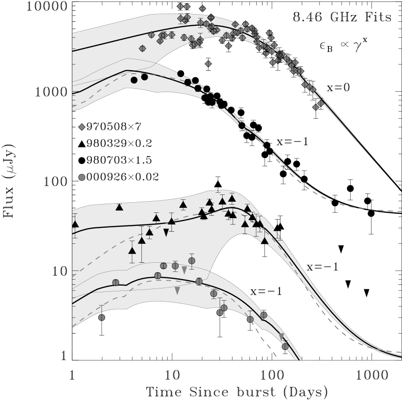
Figure 5: 8.46 GHz light curves of the four events, with the best fits (solid lines) for an assumed magnetic energy relation $\epsilon_{B}\propto\gamma^{x}$ (§5.1). The light grey envelopes are the estimated scintillation uncertainties (the 970508 scatter is not fully accounted for, but it has scatter excess at all frequencies); data that isn’t 3$\sigma$ significant is shown as 2$\sigma$ upper limits (downward triangles). 980329 has a radio host component which marginally improves the fit due to a 1.43 GHz average flux excess. In one case (970508) a constant $\epsilon_{B}$ produces the best fit (but only by 1% in the total broadband $\chi^{2}$); in the others $\epsilon_{B}\propto\gamma^{-1}$ gives the best fit. For these three, the best constant-$\epsilon_{B}$ fit is shown as a grey dashed line for comparison. The model decay for constant-$\epsilon_{B}$ is generally slightly steeper than the data in the late radio; this is especially obvious in the last few points of the 000926 light curve. A magnetic energy increase at late times flattens this decay, improving the fit.

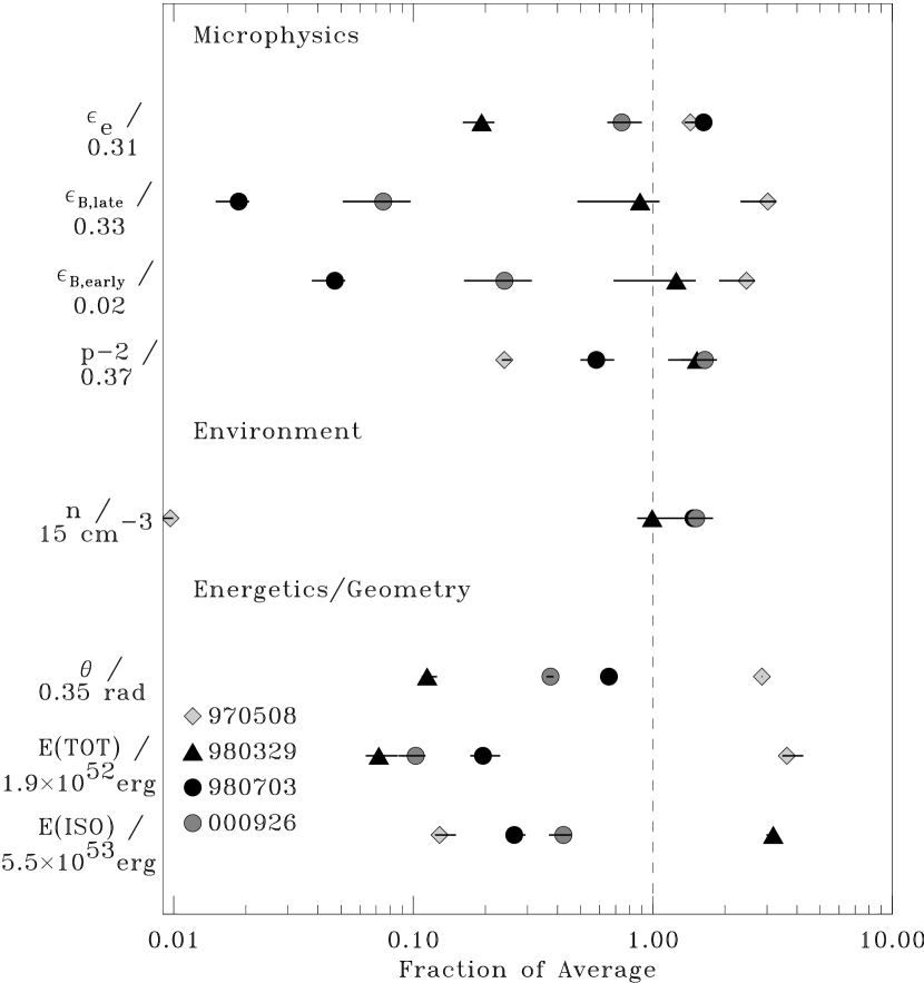
Figure 6: Parameters from the best fits assuming $\epsilon_{B}\propto\gamma^{-1}$ (see §5.1, Table 4). They are divided into 3 categories: energy & geometry (kinetic energy, collimation half-opening angle $\theta$), environment (density) and microphysics (energy partitions: $\epsilon_{e}$ for electrons, $\epsilon_{B}$ for magnetic fields, and electron energy distribution index $p$). As it varies, $\epsilon_{B}$ is presented both with its early (at fast- to slow-cooling transition) and final values. See §2 for further details concerning the fireball model’s parameters. They are presented relative to a nominal value as indicated; the error bars are statistical only, 68.3% intervals calculated via Monte Carlo bootstraps. The model uncertainties are larger, as seen in the Tables’ range of parameters that produce reasonable fits under various assumptions. This model assumption produces fits as good as (970508) or better than (980329, 980703, 000926) those assuming $\epsilon_{B}$ is constant. However, it does not fit with a universality in the microphysics. There is clearly great flexibility in the model assumptions allowed by the data, and considerable model uncertainty in the derived parameters.

Best fits for various $x$ are in Table 3. We find that $x<0$ fits as well or better than the basic model out to at least $x=-1$; the best $\epsilon_{B}\propto\gamma^{-1}$ fits including uncertainties are shown in Table 4 and Figure 6. The improvement is seen in 3 of the 4 cases, while the fit with the $x=-1$ model assumption to 970508 is only 1% worse in the total broadband $\chi^{2}$ than the basic, constant-$\epsilon_{B}$ fit. The effect of the $x=-1$ assumption on the fit to optical and X-ray data is minor. It takes a long time baseline, as in the radio, to see the spectral evolution differences; moreover the optical and X-ray are above the cooling frequency and thus have a lesser flux dependence upon $\epsilon_{B}$ (Table 2). Assuming $\epsilon_{B}\propto\gamma^{-1}$ improves the radio fits - the magnetic energy grows as the shock slows, which allows the peak to rise, flattening the late time decay, as shown in Figure 5. We note there appears to be a general trend that the radio decays are a bit shallower than the optical / X-ray, so an increasing magnetic energy improves the fit. There are other possible causes; any effect that increases the peak flux, such as an increasing energy or density, will flatten the radio decay.

For a sufficiently steep $\epsilon_{B}\propto\gamma^{x}$; $x>0$ the resulting model behaviour can no longer fit the datasets despite any compensating changes in other parameters. As the peak flux $\propto\epsilon_{B}^{1/2}$, one of the chief spectral behaviour changes is that the peak flux drops, producing steeper decays (see Table 2). This leads to a poor radio fit by $x\approx+3$, often with the radio peak flux too low in order to give an appropriate earlier peak flux relative to the optical data. The effect is stronger post-jet, and as shown in Table 3 the data for 000926 (with a clear jet break in the optical $\approx$ 2 days) does not even produce a good fit assuming $x=+1$. The extra steepening in the radio requires a later jet break than is compatible with the optical; attempts were made to compensate in fits with $t_{jet}\mathrel{\hbox{\hbox to0.0pt{\lower 2.36806pt\hbox{$\sim$}\hss}\kern 0.0pt\raise 1.72218pt\hbox{$<$}}}3$ days, but the radio could not be forced to fit. There can also be some fit difficulties at higher frequencies; these may be due to a drop in IC flux components for higher early $\epsilon_{B}$, or a change in the spectral slope from its link to the decay rates. These effects also combine; a decreased IC flux in the X-ray requires an increased synchrotron flux. In some models it is produced by overproducing the model’s optical flux and suppressing it with host extinction. The combination does not produce appropriate spectral indices both in the optical and from the optical to the X-ray.

While the $x=-1$ assumption produced improved fits, for a negative enough $x$, $\epsilon_{B}\propto\gamma^{x}$ can no longer match the data, at $x\approx-3$. For $x\ll 0$, $\epsilon_{B}$ will become unphysically high, capping at 100%, even with a reasonable early value. This occurs at $x=-4$ for 980329, where no good fit can be found with $\epsilon_{B}<100\%$ in the data range; early radio flux would decline rather than rising, in contradiction to the data (see Table 2). However, the others cannot fit before reaching that extreme. By $x=-3$, 980703’s radio peak cannot be matched. The peak frequency drops so slowly that it does not pass until quite late; a decline is produced post-jet (so too early) by pushing $\epsilon_{e}\rightarrow 1$ to maximize the energy losses. This unphysical result is also required to counteract the shallow decay at optical and X-ray frequencies. 970508 fits poorly in a similar manner, but 000926’s poor fit is again due to the definite optical break. With IC cooling dominant, the pre-jet flux is too shallow, so the jet break is pushed back earlier than the data, with a break due to the steepening associated with the change to synchrotron cooling dominance which does not match the data well.

In summary, the data does not constrain the fireball model to have a constant magnetic energy fraction $\epsilon_{B}$. Good fits are possible with both increasing and decreasing $\epsilon_{B}$, generally as strongly as $\epsilon_{B}\propto\gamma^{+1}$ through $\gamma^{-2}$. With $\gamma$ changing by a factor $\sim$ 10 over the data range, this allows an extra change in magnetic field strength by a factor of $\sim$3-10. Moreover the increasing magnetic energy with $\epsilon_{B}\propto\gamma^{-1}$ tends to improve the model fit to the radio data. As $\vec{B}\propto\gamma\epsilon_{B}^{1/2}$, a more constant level $\vec{B}\propto\gamma^{1/2}$ fits slightly better than the basic model.

5.2 An Investigation of Density Profiles $n\propto r^{S}$

The CBM density distribution is an important clue to the nature of the progenitor, with an $r^{-2}$ profile expected as the signature of a massive star (e.g. Dai & Lu, 1998; Chevalier & Li, 2000). A number of profiles have already been considered. This includes “naked GRBs” where a constant density drops to zero after a certain radius (Kumar & Panaitescu, 2000) and Ramirez-Ruiz et al. (2001)’s evolution of the afterglow through the ejecta left by a Wolf-Rayet star showing that $r^{-2}$ is a very crude approximation to the environment about a massive star. Nevertheless, most model fits do as well or better with the ISM approximation to the density profile than the Wind one (e.g., Panaitescu & Kumar, 2002), although there is one case where a Wind CBM fits and an ISM cannot (Price et al., 2002).

We investigate a wide range of density profiles, parametrized as $n\propto r^{S}$. We recalculated the equations for the model presented in §2.1 allowing for a general powerlaw density profile index $S$. This includes the changes to the radiative loss estimates, as in Cohen, Piran & Sari (1998). There are no general calculated adjustments in the equation normalizations accounting for the postshock electron distribution with a generic density profile, so we used the order of magnitude estimates (including for $\gamma$, which gives $t_{jet}$), and the estimate that from the jet expansion $t_{NR}/t_{jet}\approx\theta^{2}$.

We expect cases of $S<0$ to help constrain how sensitive the model is to the details of a mass-loss wind from the supposed progenitor star. Cases of $S<-2$ approach that of an evacuated cavity. The equations for the fireball energy from Blandford & McKee (1976) break down at $S=-4$ (see Best & Sari, 2000, for $S<-4$).

Conversely, $S>0$ models a fireball plowing into a medium that gradually increases in density. This could mimic a denser region surrounding the burst (though not a sharply bounded overdensity). For $S\gg 1$, it offers insight into the behaviour when hitting the edge of a very dense, but not sharp, shell surrounding the burst. It does not directly model the extinction column from the material, so the density would have to cut off before the material ahead would absorb all the light emitted from the shock.

Following is the the expected behaviour of the spectral breaks with general $S$. $\nu_{a}$ is for the order $\nu_{a}~{}<~{}\nu_{m}~{}<~{}\nu_{c}$. When $\nu_{a}~{}<~{}\nu_{c}~{}<~{}\nu_{m}$, it is multiplied by $(\nu_{m}/\nu_{c})^{1/2}$; other orderings have other factors.

$$\begin{array}[]{lcccc}&&t<t_{jet}&t_{jet}<t<t_{nr}&t_{nr}<t\\ \hline\cr F_{max}\propto&E^{(8+3s)/(8+2s)}n_{i}^{2/(4+s)}\epsilon_{e}^{0}\epsilon_{B}^{0.5}&t^{s/(8+2s)}&t^{-1}&t^{(2s+3)/(s+5)}\\ \nu_{a}\propto&E^{0.8(s+1)/(s+4)}n_{i}^{2.4/(s+4)}\epsilon_{e}^{-1}\epsilon_{B}^{0.2}&t^{0.6s/(s+4)}&t^{-0.2}&t^{(16s+30)/(5s+25)}\\ \nu_{m}\propto&E^{0.5}n_{i}^{0}\epsilon_{e}^{2}\epsilon_{B}^{0.5}&t^{-1.5}&t^{-2}&t^{-(4s+15)/(s+5)}\\ \nu_{c}\propto&E^{-(3s+4)/(8+2s)}n_{i}^{-4/(s+4)}\epsilon_{e}^{0}\epsilon_{B}^{-1.5}&t^{-(3s+4)/(8+2s)}&t^{0}&t^{-(2s+1)/(s+5)}\\ \end{array}$$ (4)

An increasing density ($S>0$) does not change the behaviour as greatly as a rarefaction ($S<0$). With the converse, rapid changes are expected for decreasing $S<0$, not increasing $S>0$. The reasons are illustrated by the range in densities probed and the rate at which the shock $\gamma$ slows depend upon a density profile.

Taking the observer time $t$ affected by relativistic beaming, and the relativistic energy, $E=M\gamma^{2}$ (c=1), with $M$ from the density profile $n\propto r^{S}$ the results are

$$E\propto r^{S+3}\gamma^{2},\;t\propto r\gamma^{-2}$$

Solving for $r$ gives

$$n\propto r^{S}\propto(Et)^{S/(S+4)}$$

As evident from the above equation, for $S>$ a few the rate at which density $n$ increases with observer time is weakly dependent upon $S$, despite its strong dependence on radius. As well, in the adiabatic approximation, with $E$ constant

$$\gamma\propto t^{-(S+3)/(2S+8)}$$

For $S\geq 0$, the rate of slowing only varies from from $\gamma\propto t^{-3/8}$ to $\gamma\propto t^{-1/2}$; it depends quite weakly on the density profile for $S$ larger than a few.

Moreover, in our model, the post-jet shock evolution is not sensitive to density (since it is stopped and expands laterally) until the nonrelativistic transition. Changes in the parameters to maintain the same jet break for different $S$ may make the nonrelativistic transition come at a somewhat different time, but the effect is not dramatic. The question becomes whether the model with a given $S$ can reproduce the behaviour pre-jet. To examine this, we choose the two datasets with sufficient data for well constrained jet break times. GRB 970508, which was well fit with near-isotropy, and GRB 000926, with a sharp jet break seen in the optical, are most useful to constrain possible model fits for various $S$. The others had more limited optical data, where jet breaks are generally most obvious, as it was either sparsely sampled or partly masked by a bright host. (In §4 we note that the GRB 980703 dataset could be fit equally well by ISM and Wind-like density profiles; clearly at least some very good datasets do not constrain $n(r)$.)

We have seen cases where $n\propto r^{-2}$ densities can fit the data, but it is difficult to even marginally fit models with as steep a gradient as $r^{-2.5}$ (see the best fits in Table 5). For 000926, we could not find a satisfactory fit with $r^{-2.5}$, as no good fit was possible with a jet break. The peak flux declines rapidly prejet; if it scales to fit the early optical it is low by the jet break, then too low in the radio. The radio model’s decay begins too early due to $\nu_{a}$’s rapid decline as the shock moves into less dense material. GRB 970508 is also not well fit by $n\propto r^{-2.5}$. Its $r^{-2.5}$ model with the best $\chi^{2}$ in Table 5 has an unphysical $\epsilon_{B}=100\%$, giving high initial spectral breaks $\nu_{a}$ and $\nu_{m}$ as these drop quickly. The peak is high early (as it drops quickly); the spectrum from the peak to the optical frequencies is steeper than in the ISM case. That steepness out to the X-ray frequencies causes that model to underpredict the X-ray flux. The best 970508 model for $r^{-2.5}$ under the constraint that $\epsilon_{B}<100\%$ does not fit the radio data; its predicted flux rises and falls too sharply as $\nu_{a}$ and $\nu_{m}$ fall rapidly.

As mentioned above, for an increasing density gradient the shock slows rapidly compared to the constant density case, and the resulting changes in $n$ seen by the shock are gradual. As a result, 970508 and 000926 can both be fit with $S\approx 10$ (Table 5). For 000926, the increasing density leads to a more rapid nonrelativistic transition, improving the fit somewhat relative to the constant density case. Further changes will go too far; the fit becomes marginal around $S=12$ where the best fit models overestimate the early radio flux. 970508 has no visible jet break, and is not sensitive to $S$ even for values exceeding $S\mathrel{\hbox{\hbox to0.0pt{\lower 2.36806pt\hbox{$\sim$}\hss}\kern 0.0pt\raise 1.72218pt\hbox{$>$}}}10$. Pushing to extreme $S$ to discover how far the assumptions can fit the 970508 data (eventually the gradient would make the nonrelativistic transition come too early) is of limited value; GRB 970508’s data is not very sensitive to an increasing CBM density gradient.

In summary, while the data may sometimes accomodate an $r^{-2}$ CBM, it does not fit an extreme blown-out density $r^{-2.5}$. But a shock plowing into a denser region cannot be easily excluded by the data. This is not the same as a sudden jump in density, but a gradual, continuous increase $n\propto r^{S}$, for $S\gg 1$, which is not very realistic but may roughly mimic a dense but not sharp shell of material (perhaps ejecta from the progenitor). We conclude that the fireball model data fits are not very sensitive to increasing density gradients.

6 Improving Observational Constraints

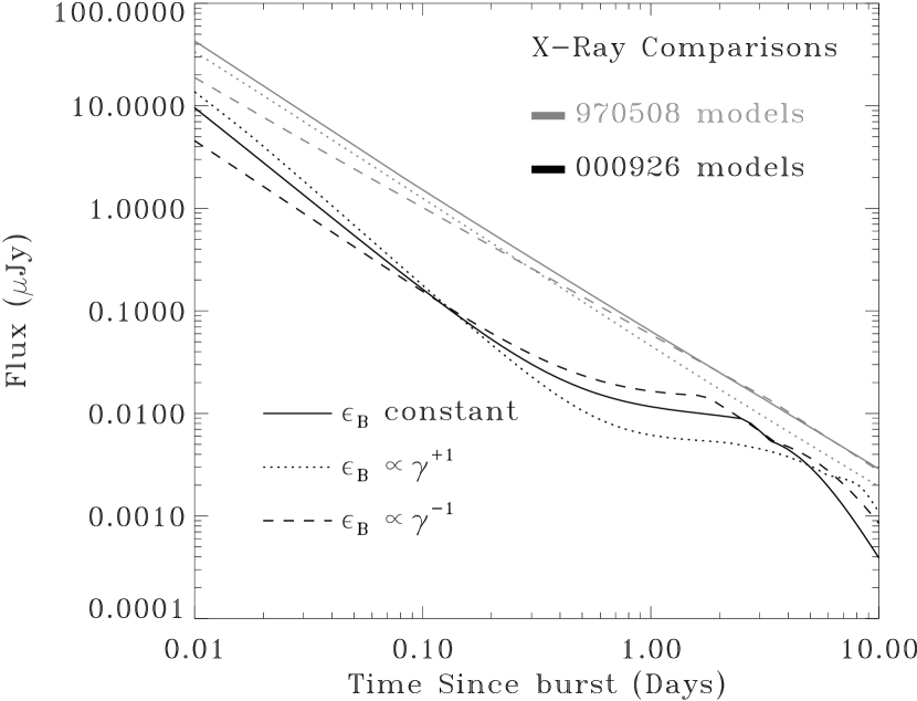
Figure 7: Comparison of model X-ray lightcurves for several equally acceptable model fits. The lightcurves are for a frequency of $6\times 10^{17}$Hz (nominal for Swift), and show the good fits for GRBs 970508 and 000926 with the basic model as well as with the assumption that the magnetic energy fraction $\propto\gamma^{\pm 1}$. While the models are close around the times of the X-ray observations ($\sim$ days), they diverge at early times, with a spread of several $\mu$Jy at 0.01-0.03 days. Moreover, in the case of 000926, there is significant IC upscattered flux, which gives different peak passage times under the differing model assumptions. Early, sensitive, densely sampled lightcurves such as those expected from Swift would determine if we are modelling the X-ray flux, including the upscattered IC photons, correctly.

In previous sections (§5.1, §5.2), we found good fits to the data under different assumptions ($\epsilon_{B}\propto\gamma^{-1}$, $\gamma^{+1}$; $n\propto r^{\sim 10}$, $r^{-1}$), as reasonable as the good fits derived from the basic model of §2.1. The datasets will tolerate widely differing assumptions since the fits need only match up with data over a limited range of frequencies and times, and there are significant degeneracies between parameters and model assumptions. For example, the decay rate depends upon the spectral index as well as the assumed $n(r)$ or $\epsilon_{B}(\gamma)$. We cross-compared these good fits with those of the basic model, checking spectra from 0.01 to 300 days to see the best ways of distinguishing them. The fitted models diverge in spectral and temporal regions far from the data, as shown in Figures 7 and 8, which highlight the most promising areas for improved constraints: longer and more sensitive X-ray and submillimeter observations.

X-ray lightcurves of some of the acceptable fits are extended to early times for comparison in Figure 7. Sets of acceptable fits for two events are shown to demonstrate that the fits in all events diverge by factors of up to three at early times; fluxes of equally acceptable fits may be 3 $\mu$Jy or 10 $\mu$Jy at 0.01-0.03 days. The sensitivity of INTEGRAL’s instruments would not be able to distinguish them, but more sensitive X-ray instruments on later $\gamma$-ray missions such as Swift may. Figure 7 includes a case with an upscattered IC flux component, whose peak passage timing gives different curvatures to the light curves. Dense, and preferably multifrequency (the IC peak can be seen in the spectrum), X-ray lightcurves would break the degeneracy between synchrotron or IC flux as the X-ray source.

Observations of the broadband peak beyond the radio may be most promising. Figure 8 shows examples of the submm lightcurves resulting from various acceptable fits found in this work; there are a variety of peak levels that subsequently match the radio peak level. The peak is in the mid-IR or submm for most of the observable afterglow, from about a day to a month. It can rise or fall for a variety of reasons (energy losses, jet break, $n(r)$, $\epsilon_{B}(\gamma)$), with details dependent upon the assumptions. These lead to models diverging in submm peak height by up to 10 mJy at fractions of a day ($\approx$ mJy in the mid-IR). Improved submm instruments are expected to reach appropriate sensitivities soon. The ALMA array, to be partially on-line by 2006 and completed by 2010, is expected to give fractional mJy sensitivity in a few minutes. Its observations could seriously constrain the peak’s behaviour.

More NIR observations will be of use; in §5.1 we noted that some fits break down where host extinction and $p$ could no longer produce appropriate spectral indices both in the optical and from the optical to the X-ray. With NIR data, host extinction is better constrained, spectral requirements constrain $p$ and allowed model assumptions can be better distinguished by their temporal behaviours for that $p$.

Finally, earlier optical observations are becoming available now (e.g. GRB 021004 Fox (2002), GRB 021211 Fox & Price (2002)) and will be of some use. However, at such early times the dominant optical emission should not be due to the synchrotron emission from a forward shock into the external medium; reverse shocks (as likely seen in the 990123 optical flash, Sari & Piran (1999a); Mészáros & Rees (1999)) and internal shocks may produce the early optical flux. This will allow further constraints, but not necessarily to the same parameters. We may be seeing in GRB 021004 that the forward shock dominates only after $\approx$ 0.1 days, and the rise of its peak may be masked by the reverse shock (Kobayashi & Zhang, 2003; Uemura et al., 2003).

Thus, the behaviours exhibited by good fits (under various model assumptions) to the datasets to date may be distinguishable in the near future, especially by densely sampled X-ray lightcurves, and observations of the peak at frequencies above the radio.

7 Conclusions

We fit four well-studied bursts with extensive radio through X-ray afterglow datasets to a fireball model with simple assumptions concerning the microphysics and environment. We find a range of reasonable environmental and geometrical parameters. We find all four fit best with a constant density medium, one with a value similar to the Milky Way’s ISM density, $n\approx 0.2$cm^-3, the other three typical of diffuse clouds $n\approx 20$cm^-3. Their kinetic energies are comparable to the total GRB $\gamma$-ray energy. The collimation varies from near-isotropy to a half-angle of 0.04 radians.

We also find a striking diversity in the fitted microphysical parameter values, far beyond the statistical uncertainties. The electron energy distribution index varies from $p=2.1-2.9$ and the magnetic energy fraction varies from 0.2% to 25%. As shock physics should depend merely on shock strength, we investigated whether the spread could be due to model uncertainty, but did not find a set of assumptions which fit the data via universal microphysics parameters.

We allowed for changes to be made to the model assumptions: $\epsilon_{B}\propto\gamma^{x}$ and independently $n\propto r^{S}$. We find considerable flexibility in the values of $x$ and $S$ that can still produce reasonable fits: $\epsilon_{B}\propto\gamma^{x}$; $-2\leq x\leq+1$ and $n\propto r^{S}$, with $S>-2$ through $S\gg 1$. Moreover, some parameter values change by up to an order of magnitude when the assumptions underlying the model are altered. Clearly, even the results of very good fits are not unique and the parameters cannot be taken at face value. The model assumptions are not strongly constrained by the datasets available to date. With this model uncertainty, the evidence for massive stellar progenitors from other sources (positions within hosts, possible SN associations, see Mészáros, 2002) is not hard to reconcile with the lack of clear $n\propto r^{-2}$ wind signatures in the best fits. Massive stars may not produce a true $r^{-2}$ profile, or its effect upon the spectrum could be masked by an inaccuracy in other model assumptions.

Finally, we compared the spectral evolution of the range of acceptable fits with differing assumptions to identify observational strategies that would produce better constraints. Two areas are most promising. First, as for now a good fit need only line up with a small time range of X-ray observations, the Swift satellite’s expected early, well-sampled X-ray lightcurves will better constrain the spectral evolution (as well as the IC upscatters of photons to the X-ray band and their consistency with the synchrotron model). As well, the peak has only been definitively observed at radio frequencies, passing through the mid-IR and submm during most of the afterglow. New submm instruments such as ALMA should increase the reach of direct peak detections. This will constrain the peak flux evolution, which is sensitive to the model assumptions.

In the future it would be useful to investigate further constraints upon the assumptions. These might include variable energy $E(t)$ (under investigation in the context of events such as 021004, e.g., Heyl & Perna, 2003), and the possibility that the electron energy (parameterized by $\epsilon_{e}$), or their acceleration (parameterized by the powerlaw index $p$), could vary with shock strength.

Table 1: Fit parameters of the best models with simple assumptions

$\chi^{2}$	DOF	$t_{cm}$	$t_{jet}$	$t_{NR}$	$E$	$E$	$\theta_{jet}$	$n$	A(V)	$p$	$\epsilon_{e}$	$\epsilon_{B}$
					$t_{cm}$	1 day	rad	cm-3	host			%
GRB 970508
596	257	0.082	183	203	3.7${}^{+0.1}_{-0.1}$	1.6	0.84${}^{+0.03}_{-0.03}$	0.20${}^{+0.01}_{-0.02}$	0.14${}^{+0.02}_{-0.02}$	2.1223${}^{+0.003}_{-0.0008}$	0.342${}^{+0.008}_{-0.01}$	25.0${}^{+0.6}_{-2}$
GRB 980329
115	90	6.1	0.12	70	126${}^{+6}_{-6}$	170	0.036${}^{+0.002}_{-0.004}$	20${}^{+5}_{-5}$	1.9${}^{+0.2}_{-0.1}$	2.88${}^{+0.1}_{-0.2}$	0.12${}^{+0.02}_{-0.02}$	17${}^{+3}_{-3}$
GRB 980703
170	147	1.4	3.4	50	11.8${}^{+0.8}_{-2}$	13	0.234${}^{+0.02}_{-0.007}$	28${}^{+4}_{-3}$	1.15${}^{+0.08}_{-0.06}$	2.54${}^{+0.04}_{-0.1}$	0.27${}^{+0.03}_{-0.03}$	0.18${}^{+0.04}_{-0.03}$
GRB 000926
138	93	3.4	2.6	79	12${}^{+2}_{-2}$	15	0.162${}^{+0.007}_{-0.004}$	16${}^{+3}_{-3}$	0.022${}^{(<0.037)}\tablenotemark{c}$	2.79${}^{+0.05}_{-0.04}$	0.15${}^{+0.01}_{-0.01}$	2.2${}^{+0.5}_{-0.6}$

Note. — Statistical uncertainties are given for the primary (employed in the fit) parameters; the other columns are derived from the fitted values. The quoted uncertainties are produced via the Monte Carlo bootstrap method with 1000 trials to generate the parameter distribution. The values bracket the resulting 68.3% confidence interval. These error bars do not include uncertainties in the model itself. The model uncertainties are larger than the statistical uncertainties, as demonstrated from the range of parameters that produce reasonable fits under various assumptions.

Table 2: Model Flux Dependences With $\epsilon_{B}\sim\gamma^{x}$

Spectral Region	Parameters	$t$, $t<t_{jet}$	$t$, $t>t_{jet}$
For $\nu_{a}~{}<~{}\nu_{m}~{}<~{}\nu_{c}$
$\nu<\nu_{a}$	$E^{0.5}n^{-0.5}\epsilon_{e}\epsilon_{B}^{0}$	$t^{0.5}$ $t^{0x}$	$t^{0}$ $t^{0x}$
$\nu_{a}<\nu<\nu_{m}$	$E^{0.83}n^{0.5}\epsilon_{e}^{-0.67}\epsilon_{B}^{0.33}$	$t^{0.5}$ $t^{-0.13x}$	$t^{-0.33}$ $t^{-0.17x}$
$\nu_{m}<\nu<\nu_{c}$	$E^{1.35}n^{0.5}\epsilon_{e}^{1.4}\epsilon_{B}^{0.85}$	$t^{-1.05}$ $t^{-0.32x}$	$t^{-2.4}$ $t^{-0.43x}$
$\nu_{c}<\nu$	$E^{1.1}n^{0}\epsilon_{e}^{1.4}\epsilon_{B}^{0.1}$	$t^{-1.3}$ $t^{-0.04x}$	$t^{-2.4}$ $t^{-0.05x}$
For $\nu_{a}~{}<~{}\nu_{c}~{}<~{}\nu_{m}$
$\nu<\nu_{a}$	$E^{0}n^{-1}\epsilon_{e}^{0}\epsilon_{B}^{-1}$	$t^{1}$ $t^{0.38x}$	$t^{1}$ $t^{0.5x}$
$\nu_{a}<\nu<\nu_{c}$	$E^{1.17}n^{0.83}\epsilon_{e}^{0}\epsilon_{B}$	$t^{0.17}$ $t^{-0.38x}$	$t^{-1}$ $t^{-0.5x}$
$\nu_{c}<\nu<\nu_{m}$	$E^{0.75}n^{0}\epsilon_{e}^{0}\epsilon_{B}^{-0.25}$	$t^{-0.25}$ $t^{0.09x}$	$t^{-1}$ $t^{0.13x}$
$\nu_{m}<\nu$	$E^{1.1}n^{0}\epsilon_{e}^{1.4}\epsilon_{B}^{0.1}$	$t^{-1.3}$ $t^{-0.04x}$	$t^{-2.4}$ $t^{-0.05x}$

Table 3: Fit parameters for the best models with $\epsilon_{B}=K\gamma^{x}$

$x$	$\chi^{2}$	DOF	$t_{cm}$	$t_{jet}$	$t_{NR}$	$E$	$E$	$n$	$p$	$\epsilon_{B,\%}$	$K$=$\epsilon_{B,\%}$/$\gamma^{x}$	$\epsilon_{e}$	$\theta$
			(d)	(d)	(d)	$t_{cm}$	1 day	cm-3		1 day
GRB 970508
$+2$	945	257	1.7	223	223	1.6	1.8	0.87	2.23	MAX	2.2	0.19	ISO
$+1$	695	257	0.57	322	322	1.8	1.5	0.21	2.20	80	8.2	0.24	ISO
$0$	596	257	0.082	183	203	3.7	1.6	0.20	2.12	25	25	0.34	0.84
$-1$	600	257	0.028	246	246	7.1	1.6	0.15	2.09	22	220	0.45	ISO
-2	569	257	0.0015	289	289	27	1.5	0.10	2.07	21	2400	0.59	ISO
-2	703	257	0.0011	498	498	13	2.0	0.032	2.14	MAX	5.9e4	0.24	ISO
GRB 980329
+4	112	90	6.5	76	76	2.9	4.7	220	2.31	21	0.021	0.23	ISO
+1	117	90	0.30	1.1	151	4100	3900	150	2.0007	64	4.7	0.027	0.075
0	115	90	6.1	0.12	70	130	170	20	2.88	17	17	0.12	0.036
-1	107	90	0.66	0.16	79	174	170	15	2.56	3.0	29	0.061	0.040
-4	114	90	-	0.38	73	50	27	6.4	2.35	MAX	2.7e13	0.090	0.064
-4	124	90	-	0.45	83	2000	35	6.9	2.43	MAX	1.2e13	0.074	0.066
GRB 980703
+3	230	147	3.4	121	121	0.74	1.2	2.1	2.13	MAX	1.3	0.39	ISO
+1	194	147	1.3	75	85	1.4	1.6	1.2	2.05	MAX	13	0.68	0.83
0	170	147	1.4	3.4	50	12	13	28	2.54	0.18	0.18	0.27	0.23
-1	165	147	1.2	3.5	52	14	16	22	2.21	0.083	0.62	0.51	0.23
-3	180	147	0.026	1.7	76	120	12	2.3	2.06	0.42	370	1	0.13
-3	174	147	0.044	1.9	76	170	20	3.8	2.06	0.16	140	1	0.14
-(4+)	180	147	0.36	73	93	3.8	1.9	0.51	2.03	MAX	1.5e6	0.92	0.78
GRB 000926
+1	209	93	6.0	8.2	80	3.8	5.3	14	2.88	20	2.5	0.15	0.28
0	138	93	3.4	2.6	79	12	15	16	2.79	2.2	2.2	0.15	0.16
-1	127	93	3.4	1.7	80	23	32	23	2.61	0.26	2.5	0.23	0.13
-3	198	93	0.043	0.79	100	28	15	2.4	2.18	11	1.5e4	0.20	0.079
-3	217	93	0.25	0.25	111	85	66	2.7	2.21	6.6	1.0e4	0.15	0.042

Note. — Certain items reach limits indicated in the table. Collimations reaching the isotropic limit of $\theta\approx 1$ are noted as “ISO”. Some magnetic energy fractions reach the physical limit of 100% of the shock energy, noted as “MAX”; for such models where the magnetic energy fraction drops with the shock $\gamma$ ($x>0$), $\epsilon_{B}$ is in the physical range over much of the data’s time range, the other such models are pinned at this limit over the entire dataset. Blank times $t_{cm}$ for the end of fast cooling indicate that the afterglow model formally has the transition much earlier than any afterglow data, in the range of prompt emission.

Table 4: Best fits assuming $\epsilon_{B}\propto\gamma^{-1}$

$\chi^{2}$	DOF	$t_{cm}$	$t_{jet}$	$t_{NR}$	$E_{52}$	$E_{52}$	$\theta_{jet}$	$n$	A(V)	$p$	$\epsilon_{e}$	$\epsilon_{B,\%}$	$\epsilon_{B,\%}$	$\epsilon_{B,\%}$
		(d)	(d)	(d)	$t_{cm}$	1 d	rad	cm-3	host			$t_{cm}$	1 d	$t_{NR}$
GRB 970508
600	257	0.028	246	246	7.1${}^{+1.2}_{-0.3}$	1.6	ISO	0.146${}^{+0.004}_{-0.04}$	0.09${}^{+0.03}_{-0.04}$	2.088${}^{+0.006}_{-0.002}$	0.45${}^{+0.02}_{-0.03}$	4.8${}^{+0.4}_{-1.1}$	22	100
GRB 980329
107	90	0.66	0.16	79	174${}^{+6}_{-11}$	170	0.040${}^{+0.004}_{-0.002}$	15${}^{+4}_{-2}$	1.46${}^{+0.09}_{-0.08}$	2.56${}^{+0.05}_{-0.08}$	0.061${}^{+0.008}_{-0.01}$	2.4${}^{+0.5}_{-1.1}$	3.0	29
GRB 980703
165	147	1.2	3.5	52	14${}^{+2}_{-1}$	16	0.23${}^{+0.02}_{-0.01}$	22${}^{+4}_{-3}$	1.25${}^{+0.05}_{-0.05}$	2.21${}^{+0.04}_{-0.03}$	0.51${}^{+0.04}_{-0.06}$	0.091${}^{+0.010}_{-0.018}$	0.083	0.62
GRB 000926
127	93	3.4	1.7	80	23${}^{+2}_{-3}$	32	0.131${}^{+0.004}_{-0.005}$	23${}^{+4}_{-5}$	0.036(<0.063)	2.61${}^{+0.08}_{-0.2}$	0.23${}^{+0.05}_{-0.03}$	0.47${}^{+0.14}_{-0.15}$	0.26	2.5

Note. — Statistical uncertainties are given for the primary (employed in the fit) parameters; the other columns are derived from the fitted values. The quoted uncertainties are produced via the Monte Carlo bootstrap method with 1000 trials to generate the parameter distribution. The values bracket the resulting 68.3% confidence interval. These error bars do not include uncertainties in the model itself. The model uncertainties are larger than the statistical uncertainties, as demonstrated from the range of parameters that produce reasonable fits under various assumptions.

Table 5: Fit parameters for the best models with $n=n_{i}(r/r_{i})^{S}$

$S$	$\chi^{2}$	DOF	$t_{cm}$	$t_{jet}$	$t_{NR}$	$E_{cm}$	$E$	$n_{18}$	$n$	$R_{18}$	$n$	$R_{18}$	$p$	$\epsilon_{B}$	$\epsilon_{e}$	$\theta$
			(d)	(d)	(d)		1 d		1 d	1 d	100 d	100 d		(%)
GRB 970508
12.5	617	257	0.0044	52	52	8.3	0.75	0.087	0.14	1.0	1.9	1.3	2.08	3.2	0.56	ISO
0	596	257	0.082	183	203	3.7	1.6	0.20	0.20	0.57	0.20	2.7	2.12	25	0.34	0.84
-2.5	832	257	4.5	$1.3\times 10^{5}$	$1.3\times 10^{5}$	0.44	0.50	0.021	3.3	0.13	0.0023	2.4	2.32	MAX	0.052	ISO
-2.5	1012	257	3.8	$6.2\times 10^{3}$	$6.2\times 10^{3}$	1.8	2.6	0.25	170	0.0074	0.30	0.93	2.28	0.095	0.20	ISO
GRB 000926
12	160	93	1.8	1.6	23	4.3	5.4	$9.4\times 10^{7}$	70	0.31	320	0.35	2.14	0.34	0.35	0.27
12	141	93	2.2	2.2	26	7.5	9.7	$1.9\times 10^{7}$	73	0.35	530	0.42	2.64	0.026	0.31	0.29
10	135	93	2.1	1.9	26	6.7	8.2	$1.6\times 10^{7}$	92	0.30	560	0.36	2.45	0.046	0.26	0.27
0	138	93	3.4	2.6	79	12	15	16	16	0.29	16	0.37	2.79	2.2	0.15	0.16
-2.5	196	93	0.35	$4.7\times 10^{7}$	$4.7\times 10^{7}$	48	47	0.17	1.2	0.46	0.00056	9.9	2.88	0.046	0.033	ISO

Note. — Certain items reach limits indicated in the table. Collimations reaching the isotropic limit of $\theta\approx 1$ are noted as “ISO”. In one model the magnetic energy fraction reaches the physical limit of 100% of the shock energy, noted as “MAX”. The densities given at 1 and 100 days give an idea of the range of density probed in the model. These are calculated post-fit; the fit uses scalings based upon the density powerlaw, not a density calculation at each time.

Table 6: Model Flux Dependences With $n=n_{i}(r/r_{i})^{S}$

Spectral Region	Parameters	$t$, $t<t_{jet}$	$t$, $t>t_{NR}$
For $\nu_{a}~{}<~{}\nu_{m}~{}<~{}\nu_{c}$
$\nu<\nu_{a}$	$E^{\frac{2}{4+s}}n_{i}^{\frac{-2}{4+s}}\epsilon_{e}\epsilon_{B}^{0}$	$t^{\frac{2}{4+s}}$	$t^{\frac{-2(s+1)}{s+5}}$
$\nu_{a}<\nu<\nu_{m}$	$E^{\frac{10+4s}{12+3s}}n_{i}^{\frac{2}{4+s}}\epsilon_{e}^{\frac{-2}{3}}\epsilon_{B}^{\frac{1}{3}}$	$t^{\frac{s+2}{s+4}}$	$t^{\frac{10s+24}{3s+15}}$
$\nu_{m}<\nu<\nu_{c}$	$E^{\frac{p}{4}+\frac{12+5s}{16+4s}}n_{i}^{\frac{2}{s+4}}\epsilon_{e}^{p-1}\epsilon_{B}^{\frac{p+1}{4}}$	$t^{\frac{-3p}{4}+\frac{12+5s}{16+4s}}$	$t^{\frac{8s+21-(4s+15)p}{2(s+5)}}$
$\nu_{c}<\nu$	$E^{\frac{p+2}{4}}n_{i}^{0}\epsilon_{e}^{p-1}\epsilon_{B}^{\frac{p-2}{4}}$	$t^{\frac{-3p+2}{4}}$	$t^{\frac{6s+20-(4s+15)p}{2(s+5)}}$
For $\nu_{a}~{}<~{}\nu_{c}~{}<~{}\nu_{m}$
$\nu<\nu_{a}$	$E^{\frac{-s}{4+s}}n_{i}^{\frac{-12}{12+3s}}\epsilon_{e}^{0}\epsilon_{B}^{-1}$	$t^{\frac{4}{4+s}}$	$t^{\frac{8s+10}{3s+15}}$
$\nu_{a}<\nu<\nu_{c}$	$E^{\frac{14+6s}{12+3s}}n_{i}^{\frac{10}{12+3s}}\epsilon_{e}^{0}\epsilon_{B}$	$t^{\frac{2+3s}{12+3s}}$	$t^{\frac{2s+5}{2s+10}}$
$\nu_{c}<\nu<\nu_{m}$	$E^{\frac{3}{4}}n_{i}^{0}\epsilon_{e}^{0}\epsilon_{B}^{\frac{-1}{4}}$	$t^{\frac{1}{4}}$	$t^{\frac{-s+5}{s+5}}$
$\nu_{m}<\nu$	$E^{\frac{p+2}{4}}n_{i}^{0}\epsilon_{e}^{p-1}\epsilon_{B}^{\frac{p-2}{4}}$	$t^{\frac{-3p+2}{4}}$	$t^{\frac{6s+20-(4s+15)p}{2(s+5)}}$

Figure 8: Comparison of model submillimeter lightcurves for several equally acceptable model fits. The lightcurves are for a frequency of 320 GHz (nominal center of an ALMA atmospheric window), and show the good fits for GRBs 970508 and 000926 with the basic model as well as with the assumption that the density $\propto r^{-1}$,$r^{\approx 10}$. Present sensitivities of $\approx$1 mJy, attainable only on timescales $\sim$ day, are insufficient to distinguish between the variety of peak levels that subsequently match the radio peak. This spread in peak levels is due to differing peak behaviours (rising or falling) whose details depend upon factors such as energy losses, jet break, $n(r)$, or $\epsilon_{B}(\gamma)$. The early model divergences due to density profile are of $\sim$ 3 mJy; with models with differing magnetic energy fraction ($\epsilon_{B}(\gamma)$) it is up to 10 mJy. These early differences could be resolved with improved submm instruments soon. The ALMA array, to be partially on-line by 2006 and completed by 2010, is expected to give fractional mJy sensitivity in a few minutes, which could distinguish amongst these.

References

- Achterberg et al. (2001) Achterberg, A., Gallant, Y. A., Kirk, J. G., and Guthmann, A. W. 2001, MNRAS, 328, 393.
- Beloborodov (2000) Beloborodov, A. M. 2000, ApJ, 539, L25.
- Berger et al. (2003) Berger, E., Cowie, L. L., Kulkarni, S. R., Frail, D. A., Aussel, H., and Barger, A. J. 2003, ApJ, 588, 99.
- Berger, Kulkarni & Frail (2001) Berger, E., Kulkarni, S. R., and Frail, D. A. 2001, ApJ, 560, 652.
- Berger et al. (2001) Berger, E. et al. 2001, GCN notice 1182.
- Bessell (1979) Bessell, M. S. 1979, PASP, 91, 589.
- Best & Sari (2000) Best, P. and Sari, R. 2000, Physics of Fluids, 12, 3029.
- Blandford & McKee (1976) Blandford, R. D. and McKee, C. F. 1976, Phys. of Fluids, 19, 1130.
- Bloom, Frail & Sari (2001) Bloom, J. S., Frail, D. A., and Sari, R. 2001, AJ, 121, 2879.
- Bremer et al. (1998) Bremer, M., Krichbaum, T. P., Galama, T. J., Castro-Tirado, A. J., Frontera, F., Van Paradijs, J., Mirabel, I. F., and Costa, E. 1998, A&A, 332, L13.
- Chary et al. (1998) Chary, R. et al. 1998, ApJ, 498, L9+.
- Chevalier (1999) Chevalier, R. A. 1999, ApJ, 511, 798.
- Chevalier & Li (2000) Chevalier, R. A. and Li, Z. 2000, ApJ, 536, 195.
- Coburn & Boggs (2003) Coburn, W. and Boggs, S. E. 2003, Nature, 423, 415.
- Cohen, Piran & Sari (1998) Cohen, E., Piran, T., and Sari, R. 1998, ApJ, 509, 717.
- Costa et al. (1997) Costa, E. et al. 1997. IAU circular 6649.
- Dai & Lu (1998) Dai, Z. G. and Lu, T. 1998, MNRAS, 298, 87.
- Dai & Lu (2002) Dai, Z. G. and Lu, T. 2002, ApJ, 565, L87.
- Dall et al. (2000) Dall, T. et al. 2000, GCN notice 804.
- Fox (2002) Fox, D. W. 2002, GCN notice 1564.
- Fox & Price (2002) Fox, D. W. and Price, P. A. 2002, GCN notice 1731.
- Frail et al. (2002) Frail, D. A. et al. 2002, ApJ, 565, 829.
- Frail et al. (2001) Frail, D. A. et al. 2001, ApJ, 562, L55.
- Frail, Waxman & Kulkarni (2000) Frail, D. A., Waxman, E., and Kulkarni, S. R. 2000, ApJ, 537, 191.
- Frail et al. (2003) Frail, D. A. et al. 2003, Submitted to ApJ; astro-ph/0301421.
- Garcia et al. (1998) Garcia, M. R. et al. 1998, ApJ, 500, L105.
- Gorosabel et al. (2000) Gorosabel, J. et al. 2000, GCN notice 803.
- Granot, Piran & Sari (1999a) Granot, J., Piran, T., and Sari, R. 1999a, ApJ, 513, 679.
- Granot, Piran & Sari (1999b) Granot, J., Piran, T., and Sari, R. 1999b, ApJ, 527, 236.
- Granot & Sari (2002) Granot, J. and Sari, R. 2002, ApJ, 568, 820.
- Hanlon et al. (2000) Hanlon, L. et al. 2000, A&A, 359, 941.
- Hanlon et al. (1999) Hanlon, L. et al. 1999, A&AS, 138, 459.
- Harrison et al. (2001) Harrison, F. A. et al. 2001, ApJ, 559, 123.
- Heyl & Perna (2003) Heyl, J. S. and Perna, R. 2003, ApJ, 586, L13.
- Hurley (2000) Hurley, K. 2000, GCN notice 802.
- Hurley et al. (2000) Hurley, K., Mazets, E., Golenetskii, S., and Cline, T. 2000, GCN notice 801.
- In ’t Zand et al. (1998) In ’t Zand, J. J. M. et al. 1998, ApJ, 505, L119.
- Katz (1994) Katz, J. I. 1994, ApJ, 432, L107.
- Kippen et al. (1998) Kippen, R. M. et al. 1998, GCN notice 143.
- Kirk & Duffy (1999) Kirk, J. G. and Duffy, P. 1999, Journal of Physics G Nuclear Physics, 25, 163.
- Kirk et al. (2000) Kirk, J. G., Guthmann, A. W., Gallant, Y. A., and Achterberg, A. 2000, ApJ, 542, 235.
- Kobayashi & Sari (2001) Kobayashi, S. and Sari, R. 2001, ApJ, 551, 934.
- Kobayashi & Zhang (2003) Kobayashi, S. and Zhang, B. 2003, ApJ, 582, L75.
- Kumar & Panaitescu (2000) Kumar, P. and Panaitescu, A. 2000, ApJ, 541, L51.
- Kumar & Piran (2000) Kumar, P. and Piran, T. 2000, ApJ, 532, 286.
- Levine, Morgan & Muno (1998) Levine, A., Morgan, E., and Muno, M. 1998. IAU circular 6966.
- Li & Chevalier (2001) Li, Z. and Chevalier, R. A. 2001, ApJ, 551, 940.
- Lyutikov, Pariev & Blandford (2003) Lyutikov, M., Pariev, V., and Blandford, R. 2003, astro-ph/0305410.
- Mészáros (2002) Mészáros, P. 2002, ARA&A, 40, 137.
- Medvedev & Loeb (1999) Medvedev, M. V. and Loeb, A. 1999, ApJ, 526, 697.
- Mészáros & Rees (1999) Mészáros, P. and Rees, M. J. 1999, MNRAS, 306, L39.
- Nakar, Piran & Granot (2003) Nakar, E., Piran, T., and Granot, J. 2003, New Astronomy, 8, 495.
- Narayan (1992) Narayan, R. 1992, Phil. Trans. Roy. Soc. London, Series A, 341, 151.
- Paczyński & Rhoads (1993) Paczyński, B. and Rhoads, J. 1993, ApJ, 418, L5.
- Panaitescu & Kumar (2001a) Panaitescu, A. and Kumar, P. 2001a, ApJ, 560, L49.
- Panaitescu & Kumar (2001b) Panaitescu, A. and Kumar, P. 2001b, ApJ, 554, 667.
- Panaitescu & Kumar (2002) Panaitescu, A. and Kumar, P. 2002, ApJ, 571, 779.
- Panaitescu, Mészáros & Rees (1998) Panaitescu, A., Mészáros, P., and Rees, M. J. 1998, ApJ, 503, 314.
- Piro et al. (1998) Piro, L. et al. 1998, A&A, 331, L41.
- Price et al. (2002) Price, P. A. et al. 2002, ApJ, 572, L51.
- Ramirez-Ruiz et al. (2001) Ramirez-Ruiz, E., Dray, L. M., Madau, P., and Tout, C. A. 2001, MNRAS, 327, 829.
- Rhoads (1999) Rhoads, J. E. 1999, ApJ, 525, 737.
- Rossi & Rees (2003) Rossi, E. and Rees, M. J. 2003, MNRAS, 339, 881.
- Rybicki & Lightman (1979) Rybicki, G. B. and Lightman, A. P. 1979, Radiative processes in astrophysics, (New York: Wiley-Interscience).
- Sari (1997) Sari, R. 1997, ApJ, 489, L37.
- Sari & Esin (2001) Sari, R. and Esin, A. A. 2001, ApJ, 548, 787.
- Sari & Mészáros (2000) Sari, R. and Mészáros, P. 2000, ApJ, 535, L33.
- Sari & Piran (1999a) Sari, R. and Piran, T. 1999a, ApJ, 517, L109.
- Sari & Piran (1999b) Sari, R. and Piran, T. 1999b, ApJ, 520, 641.
- Sari, Piran & Halpern (1999) Sari, R., Piran, T., and Halpern, J. P. 1999, ApJ, 519, L17.
- Sari, Piran & Narayan (1998) Sari, R., Piran, T., and Narayan, R. 1998, ApJ, 497, L17.
- Schlegel, Finkbeiner & Davis (1998) Schlegel, D. J., Finkbeiner, D. P., and Davis, M. 1998, ApJ, 500, 525.
- Sokolov et al. (1998) Sokolov, V. V., Kopylov, A. I., Zharikov, S. V., Feroci, M., Nicastro, L., and Palazzi, E. 1998, A&A, 334, 117.
- Spada, Panaitescu & Mészáros (2000) Spada, M., Panaitescu, A., and Mészáros, P. 2000, ApJ, 537, 824.
- Taylor et al. (1997) Taylor, G. B., Beasley, A. J., Frail, D. A., and Kulkarni, S. R. 1997. IAU circular 6670.
- Taylor et al. (1998) Taylor, G. B. et al. 1998, ApJ, 502, L115.
- Taylor & Cordes (1993) Taylor, J. H. and Cordes, J. M. 1993, ApJ, 411, 674.
- Tokunaga (2000) Tokunaga, A. T. 2000. Allen’s Astrophysical Quantities, chapter 7. AIP, New York, 4th edition.
- Uemura et al. (2003) Uemura, M., Kato, T., Ishioka, R., and Yamaoka, H. 2003, Accepted for publication in PASJ; astro-ph 0303119.
- Walker (1998) Walker, M. A. 1998, MNRAS, 294, 307.
- Wang & Loeb (2000) Wang, X. and Loeb, A. 2000, ApJ, 535, 788.
- Weingartner & Draine (2001) Weingartner, J. C. and Draine, B. T. 2001, ApJ, 548, 296.
- Wijers & Galama (1999) Wijers, R. A. M. J. and Galama, T. J. 1999, ApJ, 523, 177.
- Yost et al. (2002) Yost, S. A. et al. 2002, ApJ, 577, 155.
- Zharikov, Sokolov & Baryshev (1998) Zharikov, S. V., Sokolov, V. V., and Baryshev, Y. V. 1998, A&A, 337, 356.