Non-radial motion and the NFW profile

The self-similar infall model (SSIM) is normally discussed in the context of radial orbits in spherical symmetry. However it is possible to retain the spherical symmetry while permitting the particles to move in Keplerian ellipses, each having the squared angular momentum peculiar to their ‘shell’. The spherical ‘shell’, defined for example by the particles turning at a given radius, then moves according to the radial equation of motion of a ‘shell’ particle. The ‘shell’ itself has no physical existence except as an ensemble of particles, but it is convenient to sometimes refer to the shells since it is they that are followed by a shell code. In this note we find the distribution of squared angular momentum as a function of radius that yields the NFW density profile for the final dark matter halo. It transpires that this distribution is amply motivated dimensionally. An effective ‘lambda’ spin parameter is roughly constant over the shells. We also study the effects of angular momentum on the relaxation of a dark matter system using a three dimensional representation of the relaxed phase space.

1 Introduction

In the paradigm of Cold Dark Matter (CDM), what have been called universal density profiles have emerged from collisionless self-gravitating numerical models in the form

$$\rho\propto r^{-\alpha}\left(1+\left(\frac{r}{r_{s}}\right)^{\beta}\right)^{-\frac{\gamma-\alpha}{\beta}},$$ (1)

where either $\alpha=1,$ $\beta=1,$ $\gamma=3$ (NFW ) or (Moore et al. (1999)) $\alpha=1.5,$ $\beta=1,$ $\gamma=3$. Noting the importance of mergers in hierarchical clustering Syer & White (Syer & White (1998)) argued for this universality as a self-regulation of a halo density profile. This is due to tidal stripping and dynamical friction acting alternately on merging satellites to flatten a steep profile and steepen a flat profile. Independently (Subramanian et al. 1999a ) gave a similar argument wherein a nested sequence of undigested cores form the profile, each with power law densities dominating only locally. However several authors have shown that N-body simulations reproduce the (NFW ) profile without the need for clumpy initial conditions and mergers (Aguilar & Merritt (1990); Huss et al. 1999a ; Huss et al. 1999b ; Moore et al. (1999); Tittley & Couchman (2000)).

The radial Self-Similar Secondary Infall model (SSIM: FG (84); Moutarde et al. (1995); HW (99)) predicts a ‘one-sided attractor’ final density profile according to (but see (Hoffman & Shaham (1985)) for a slightly different dependence on the cosmological spectral index)

$$\frac{\rho}{\rho_{c}}=\left\{\begin{array}[]{cc}\left(\frac{r}{r_{s}}\right)^{-2},&n<1\\ \left(\frac{r}{r_{s}}\right)^{-\frac{3(n+3)}{n+5}},&n>1\end{array}\right..$$ (2)

Here $n$ refers to the power spectrum of the primordial cosmological perturbations piece-wise approximated as $P\propto k^{n}$. In the range of acceptable initial conditions the variations in the predicted density logarithmic slope are small ($2\leq\frac{3(n+3)}{n+5}\leq\frac{9}{4}$). Hence the predicted central cusps are too steep compared to those found in the N-body simulations or indeed compared to observations (De Blok et al. (2001)). In a companion paper (Henriksen & Le Delliou (2002)), the SSIM is shown to admit density inflections at the centre when finite physical resolution is accounted for, but the expected flattening may not be on a large enough scale to reproduce that of the N-body simulations. Such resolution effects however may lie behind the mass resolution dependence in the results of Jing & Suto (Jing & Suto (2000)).

Recently Lokas & Hoffman (Lokas & Hoffman (2000)) have studied the consequences of abandoning the self-similar aspect of the SSIM in favour of an adiabatic invariant calculation, and of introducing a more detailed form of the initial power spectrum. However the self-similarity has been found to arise naturally in most shell code simulations (i.e. it is not an assumption) and in any case the results of Lokas & Hoffman are very close to those cited above for the SSIM. The authors conclude by suggesting that it is prominently the presence of angular momentum that flattens the central cusp.

Indeed numerous authors have emphasized the effect of an isotropic velocity dispersion ( thus of non-radial motion) in the core of collisionless haloes. Thus (Huss et al. 1999b )’s Fig. 17 shows an NFW-type density cusp flattening relative to the isothermal profile just where the velocity dispersion changes from predominantly radial to isotropic. This flattening doesn’t appear, in (Huss et al. 1999a ), for the case of pure radial force. A similar result was obtained by (Tormen et al. (1997)), and (Teyssier et al. (1997)) who also found that singular isothermal profiles arise during radial infall while isotropic velocity dispersions are associated with flatter profiles. Similarly, Moutarde et al. (Moutarde et al. (1995)) correlate flat density profiles with higher dimensionality of the available phase space during infall and they confirm the natural development of self-similarity after turn-around. Thus we are motivated to consider a simple extension of the SSIM that includes the effects of angular momentum (i.e. of each orbiting particle producing in general a smooth velocity ‘anisotropy’ — the limits being purely radial or spherically symmetric in velocity space — at each point on a spherical ‘shell’).

Such a spherical model corresponds strictly neither to reality nor to the 3D N-body simulations of cosmological dark halo fields, which display marked non-sphericity (e.g. in Huss et al. 1999a ; Huss et al. 1999b ; Moutarde et al. (1995); Teyssier et al. (1997); Tormen et al. (1997)). Some groups have even proposed a triaxial density profile to replace the spherical (NFW ) fit (Jing & Suto (2002)). We can regard the spherical model as the result of a kind of ‘coarse-graining’ or averaging in angle, but it remains unclear in principle whether the averaging before the evolution as done here is equivalent to the averaging after the evolution as done in the simulations (NFW ). In practice we simply examine to what extent the respective profiles agree.

Various authors (Ryden & Gunn (1987); White & Zaritsky (1992); Ryden (1993); Subramanian et al. 1999a , Subramanian 1999b ; Sikivie et al. (1997) ) have treated degrees of velocity anisotropy (orbital angular momentum) in the SSIM and found hints of shallow inner density cusps, and in at least one case links between the NFW inner slope and isotropic velocities (Ryden & Gunn (1987)) were found. However none of these semi-analytic treatments followed the system through relaxation by phase mixing and instability (HW (99); Merrall (2003)) to its final form. In (Ryden (1993)) the spherical symmetry was broken and the final phase space was studied but the particle orbits were confined to poloidal planes. Nevertheless slightly flatter spherically averaged density profiles were found which may reflect the correlation with higher dimensionality found above (Moutarde et al. (1995)). We pursue the possible effects of general velocity anisotropy here by the use of a spherically-symmetric shell code, whose only constraint is that the angular momentum should be zero averaged over shells.

In fact the system is made up of particles on elliptical orbits that lie in planes through the centre of the system and are isotropically distributed in angle at any point on a sphere. Thus the vector angular momentum on the sphere is zero. A spherical ‘shell’ may be defined as the set of particles at a given radius that are all at the same phase in their orbits. It might be the turn-around or apocentric phase for example. Subsequently the shell comoves with the same set of particles according to the radial equation of motion of a particle.

Because of the spherical symmetry, angular momentum has to be introduced to the particles ad hoc, after which it is conserved. This was done in (White & Zaritsky (1992)) by introducing a heuristic source term that switches off at turnaround, or in another context simply by assigning an angular momentum distribution at turn-around time (Sikivie et al. (1997)).

In this work, two forms of angular momentum are assigned at the turn-around of a given set of particles. It is convenient subsequently to speak of this angular momentum squared as being assigned to a shell, but the reality is as described above. In the next section, we will briefly explain our implementation of angular momentum in the SSIM. The effect on the density profile will be shown in Sect. 3. Sect. 4 will focus on other consequences for the SSIM’s relaxation. A brief discussion regarding mass-angular momentum correlation will be presented in Sect. 5 before a concluding discussion (Sect. 6).

2 The SSIM and Particle Angular Momentum

We seek a natural way of assigning the particle angular momentum on a shell ‘a priori’ so that our eventual agreement with the NFW density profile should not simply be an empirical fit. There are two possibilities which seem rather natural to us. The first one is to assign that distribution of angular momentum over the ‘shells’ which allows the generalized self-similarity described by Henriksen (Henriksen (1989)) to hold until shell crossing. Unfortunately this self-similarity does not carry through into the virialized system by way of a constant logarithmic derivative of the turn-around time with respect to the turn-around radius as in (FG (84)) or in (HW (99)). In fact rather than yielding a prediction for the final density profile in terms of the assigned magnitude of angular momentum as might be anticipated, we find that the permitted magnitude is so small that no essential change is produced in the relaxed density profile. This distribution will be referred to as the self-similar angular momentum profile or SSAM.

The second distribution that we consider and the one that seems to produce the most satisfying results physically is simply that given by dimensional analysis in a spherically symmetric self-gravitating system. This is simply a power law distribution and will be referred to as the power law angular momentum profile or PLAM.

2.1 The SSAM: Self-similarity with angular momentum

Following (Henriksen (1989)) the radial equation of motion may be written in the ‘Friedman’ form

$$\left(d_{\xi}S\right)^{2}-\frac{1}{S}+\frac{J^{2}}{S^{2}}=-1,$$ (3)

where we have defined the Lagrangian label (recall that for bound shells, E$<$0, hence the -1 in Eq. (3))

$$a=\frac{GM(r)}{\left|E\right|}.$$ (4)

The current radius $R(r,t)$ of a particle or spherical shell is the scaled form

$$R=aS(\xi),$$

with the self-similar independent variable defined as

$$\xi=\sqrt{\frac{2GM}{a^{3}}}\left(t-t_{0}(a)\right),$$

and $t_{0}(a)$ is the turn-around time, chosen so that at turn-around $\xi=0$. Maintaining the self-similarity of Eq.(3) requires $J^{2}$ to be constant, which yields a constraint on the square of the ‘shell angular momentum’ $j^{2}$ through the definition

$$J^{2}=\frac{j^{2}}{2GMa}.$$ (5)

This quantity may also be written using equation (4) in the form

$$J=\frac{j|E|^{1/2}}{\sqrt{2}GM},$$ (6)

which shows it to be, but for a factor $\sqrt{2}$, the ‘local’ spin parameter $\lambda$ (Peebles (1993)) expressed in terms of specific angular momentum and energy. The mass however is the entire mass inside a given shell rather than simply that of the particles constituting the shell.

The solution to Eq. (3) before shell crossing and up to turn-around is

$$\xi+\pi/4=-\sqrt{S-(S^{2}+J^{2})}+\frac{1}{2}\arcsin{\frac{2S-1}{\sqrt{1-4J^{2}}}},$$ (7)

which gives $\xi=0$ at the turn-around scale $S_{T}$ since there

$$S-(S^{2}+J^{2})=0,$$ (8)

and thus

$$2S_{T}-1=\sqrt{1-4J^{2}}.$$ (9)

At $t=0$ Eq. (7) yields the relation

$$\sqrt{\frac{2GM}{a^{3}}}t_{o}(a)=\frac{\pi}{4}+\sqrt{S_{o}-(S_{o}^{2}+J^{2})}+\frac{1}{2}\arcsin{\frac{1-2S_{o}}{\sqrt{1-4J^{2}}}},$$ (10)

where $S_{o}\equiv r/a$, the ratio of the initial radius of a ‘shell’ and its Lagrangian label. Once this latter ratio is determined the turn-around time $t_{o}$ may be found as a function of $a$. This ratio follows from Eqs. (4) and (5) once $E(r)$ and $M(r)$ are given initially, as does also the required $j^{2}(r)$. Thus this requirement of self-similarity before shell crossing leads to a natural initial correlation between $j^{2}$ and the mass inside a shell.

The expression for the initial mass inside radius $r$ for a constant density background perturbed by a power law $\rho=\rho_{b}(1+x^{-\epsilon})$ is

$$M(r)=M_{f}x^{3}\left(1+\frac{x^{-\epsilon}}{q}\right)$$ (11)

where q is defined in terms of the power-law index $\epsilon$ of the initial density perturbations

$$q=(1-\frac{\epsilon}{3})$$

, and we adopt

$$\rho=\rho_{b}\left(1+\lambda.r^{-\epsilon}\right),$$

$\lambda$ being constant. The scaled radius $x\equiv r/r_{f}$ is defined in terms of a fiducial radius ($r_{f}=\left(\lambda\right)^{\frac{1}{\epsilon}}$) and the fiducial mass is introduced as

$$M_{f}=\frac{4\pi}{3}\rho_{b}r_{f}^{3}.$$

The background density is $\rho_{b}$.

We calculate the initial specific energy of a shell in a de Sitter cosmology after the addition of the angular momentum as

$$E(r)=\frac{H^{2}r^{2}}{2}-\frac{GM(r)}{r}+\frac{j^{2}}{2r^{2}}=-\frac{4\pi G\rho_{b}\lambda}{(3-\epsilon)}r^{(2-\epsilon)}+\frac{j^{2}}{2r^{2}}.$$ (12)

Now combining Eqs. (11) and (12) in the definition (4), one finds for example

$$\frac{x}{a}=\frac{1+\sqrt{1-4J^{2}(1+qx^{\epsilon})^{2}}}{2(1+qx^{\epsilon})},$$ (13)

which yields using Eq.(5) the expression for the self-similar compatible angular momentum distribution in the SSIM as

$$\frac{j^{2}}{2GM_{f}r_{f}}=\frac{2J^{2}}{q}\leavevmode\nobreak\ x^{(4-\epsilon)}\leavevmode\nobreak\ \frac{(1+qx^{\epsilon})^{2}}{1+\sqrt{1-4J^{2}(1+qx^{\epsilon})^{2}}}.$$ (14)

Now it is immediately clear from these expressions that the imposed self-similarity can not hold beyond $x_{max}=\left((1-2J)/(2Jq)\right)^{1/\epsilon}$. The specific energy at this radius follows from Eqs. (4), (13), and (11) as

$$E=-\frac{GM_{f}}{2qr_{f}}x_{max}^{2-\epsilon},$$ (15)

and is not zero. Thus the self-similarity itself imposes an outer cut-off on the system. This does not in itself present a problem peculiar to the imposed self-similarity, since of course for the shallow initial density profile ($\epsilon<2$) the whole Universe is bound to the halo unless an arbitrary cut-off is imposed. Moreover even the steep density profile requires an arbitrary outer cut-off to define a finite mass system.

The mass at this self-similar cut-off is fortunately large compared to the fiducial mass as it becomes (11)

$$M_{max}=\frac{M_{f}}{(2Jq)^{(3/\epsilon)}}(1-2J)^{(3/\epsilon-1)},$$ (16)

and $J$ is normally in the range $10^{-3}$ to $10^{-4}$ with $\epsilon\approx 2$ in our simulations. Larger values (one might envisage adding a spin parameter value up to $\approx 3.5\times 10^{-2}$) did not permit a sufficiently large extent to allow the self-similar virialized phase to be well resolved in time (see $x_{max}$ above). The cases that avoided this numerical limit did not show any significant deviation in density or phase space from the halos formed by purely radial infall. We therefore do not dwell further on this distribution when discussing the density profiles.

2.2 PLAM: The Power Law Distribution of Angular Momentum

In this section we consider the simplest initial distribution of angular momentum (that is a correlation with the initial mass as above) that may be expected on dimensional grounds. This is the Keplerian form (the specific rotational kinetic energy is a fixed fraction $J^{2}$ of the specific binding energy)

$$\frac{\textrm{j}^{2}}{2r^{2}}=\frac{GM(r)J^{2}}{r}$$ (17)

where $J^{2}$ is again constant. As a consequence all of the equations of the previous section (including the solution for the scale factor) may be applied simply by replacing $J^{2}$ in those equations by $J^{2}x/a$ and noting that in this case the previous procedure leads to

$$\frac{x}{a}=-J^{2}+\frac{1}{1+qx^{\epsilon}}.$$ (18)

The motion before shell crossing is now no longer ‘self-similar’ in the sense of the previous section, but in fact we can see that for $J^{2}x/a$ small the situation at turn-around is little different from the purely radial motion. It is during the subsequent re-collapse that angular momentum is significant. One of our objectives is to see what form this initial correlation takes in the final relaxed halo so that it may be compared with the $\Lambda$ CDM results of Bullock et al. (Bullock et al. (2001)).

Once again the angular momentum distribution can not be maintained beyond an outer scale $x_{max}$ where now

$$x_{max}=\left(\frac{1-J^{2}}{qJ^{2}}\right)^{1/\epsilon},$$ (19)

although with $J^{2}$ small this yields a larger dynamic range than before. Eqs. (17) and (11) now yield the explicit initial angular momentum distribution as

$$\frac{j^{2}}{2GM_{f}r_{f}}=\frac{J^{2}}{q}\leavevmode\nobreak\ x^{(4-\epsilon)}(1+qx^{\epsilon}).$$ (20)

We observe that at large $qx^{\epsilon}$ this distribution tends to one for which there is a constant angular velocity as a function of initial radius. Moreover while the coefficient $J^{2}(1+qx^{\epsilon})$ is constrained to be always smaller than one, $x_{max}^{(4-\epsilon)}$ may be large. It is for this reason that $j^{2}$ may be large enough in this case to substantially alter the nature of the final collapsed halo.

In the numerical work below we present examples for $\epsilon=1.5$, the ‘shallow’ case and for $\epsilon=2.5$, the ‘steep’ case. For the SSAM $J$ is essentially the specific spin parameter ($\times 1/\sqrt{2}$) and calculations were carried out with $J\approx 1.7\times 10^{-3}$ for the shallow case and with $J\approx 6.8\times 10^{-5}$ for the steep case. These values are rather small compared to the median value of $\lambda=.05$ reported in (Peebles (1993)). This shows clearly the limitations imposed by this angular momentum distribution together with the constraint of forming a core.

For the PLAM distribution, $J^{2}$ is actually rather larger than the spin parameter wherever $x/a$ is small. The values used for $J^{2}$ were $10^{-3}$ for the shallow case and $\approx 9\times 10^{-3}$ in the steep case. These are much closer to the values for the spin parameter found in cosmological simulations. If $J^{2}$ is taken much larger than these values the outermost shells did not reach the center. In this latter event the core displayed isolated phase mixing ‘islands’ (Sikivie et al. (1997)).

3 Numerical Evolution of the PLAM Distribution to the NFW Profile

3.1 Establishment of the NFW profile

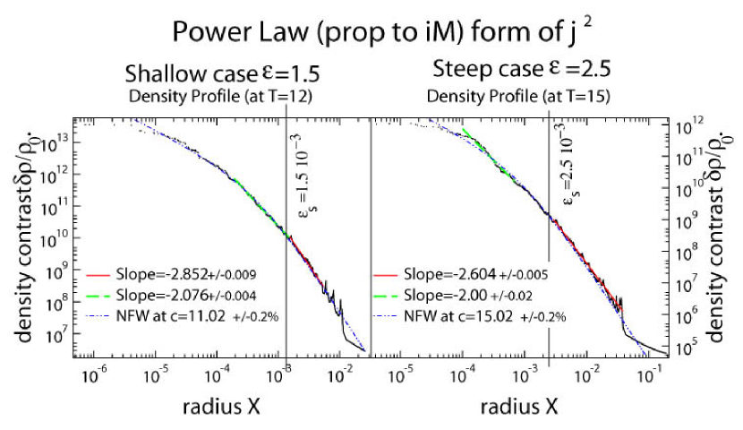
Figure 1: ‘Power law’ angular momentum (PLAM): density profiles for critical values of the angular momentum near the end of the self-similar quasi-equilibrium phase in the shallow ($\epsilon=\frac{3}{2}=1.5$) and steep ($\epsilon=\frac{5}{2}=2.5$) initial density profiles cases

We use a shell code with a semi-analytic treatment of the energy calculation (Le Delliou (2001)) to follow the development of the dark matter halo through the shell crossing phase. This code has been well tested elsewhere (Le Delliou (2001)) and is known to reproduce standard results (HW (99)).

As was indicated above the SSAM distribution did not produce density profiles that were significantly different from those found in pure radial infall. In particular the relations between the power law index of the initial density perturbation $\epsilon$ and the final density power law in the bound core were the same as those found for radial infall (FG (84); HW (99)). Thus we do not present these results here.

The PLAM initial distribution with the parameters given above evolved to cores having the density profiles shown in (Fig. 1). The time indicated on the figures is that defined in (HW (99)) and refers to the logarithmic time near the end of the self-similar infall ‘equilibrium’ phase.

The figure shows that both in the steep and shallow case the profile is no longer well fit by a power law even in the intermediate regions. Rather there is a smoothly varying convexity in the logarithmic slope that is well fit by the indicated NFW profile except in the most central regions. There a flattening occurs that is more pronounced than is accounted for by the NFW profile. Flattening is anticipated relative to the self-similar slope on general thermodynamic grounds in the coarse-graining study of (Henriksen & Le Delliou (2002)), and the presence of a central point mass (perhaps imitated here by numerically smoothed density cusps) can produce such flattened cusps (Nakano & Makino (1999)). Unfortunately our numerical resolution is too poor in this core region to say that this flattening is a physically significant result.

We also show piecewise power law fits in various regions of the figure in order to emphasize the inadequacy of a global power law fit. One sees moreover that the apparent slope does tend toward $r^{-3}$ in the external regions. The theoretical power law slope for undisturbed radial infall is $2.0$ for the shallow case and $\approx 2.14$ for the steep case. Neither of these values fits the whole density profile of these cores.

We note that the force ‘smoothing’ length $\epsilon_{s}$ occurs near the mid-point of the indicated spatial range. This does not affect the validity of the density profile inside this radius however as was established numerically and by coarse graining in (Henriksen & Le Delliou (2002)) for pure radial infall. Their interpretation of the results in terms of ‘turn-round’ relaxation of the shells is unchanged by the present extention of phase space dimensionality since, as seen in Sect. 4, relaxation still takes place mostly outside of the ‘smoothing’ length (Le Delliou (2001)). However even if the relaxation argument still holds, it cannot be made to predict the exact slope of the NFW profile. We shall examine in detail the NFW profile dependence on resolution in Sect. 3.2.

Our results ought to be compared to the results of the similar study of Hozumi et al. (Hozumi,Burkert & Fujiwara (2000)). These authors also investigate the effect of smoothly anisotropic velocity distributions (but with zero net angular momentum on shells, just as in our case) on the density profile. Instead of using a shell code however, they integrate the CBE directly starting from non-equilibrium power law density distributions. Moreover they initiate their calculation with an ‘ad hoc’ distribution function that is simply a Gaussian in each of the radial and azimuthal velocities, each Gaussian having different dispersions. In contrast we have started our simulations in this work from actual cosmological initial conditions radially, on which we have imposed rather natural distributions of angular momentum. The effect is that our collapse begins from a well-defined surface in phase space.

Despite the differences in the initial conditions, we observe that the conclusions drawn in the two works are rather similar. Their parameter $2\alpha$ is essentially our parameter $J^{-2}$ (our radial specific kinetic energy is essentially $GM/r$) which we have taken in the range $\ 100$- $1000$ for the favoured PLAM. Although the largest value used in their paper is $2\alpha=20$, because our ratio of kinetic energy to binding energy ($\approx(1+J^{2})/(1+\delta M/M)$) is much closer to unity than is theirs, the calculations are more comparable than it might seem. Hozumi et al. have not fitted their profiles with a NFW curve, but their conclusions about the central flattening resemble ours. This suggests that particle angular momentum is indeed playing a role in determining the density profiles of dark matter halos, and hence of galaxies.

We conclude then in this section that the PLAM of Eq. (20) does yield the NFW density profile over most of a dark matter halo. Moreover the required amplitude of the angular momentum does not need to exceed that likely to be provided by tidal interactions. The PLAM places the embryonic halo particles on a surface in phase space which may therefore reveal something of the tidal fields they experience near turn-around.

3.2 NFW and resolution

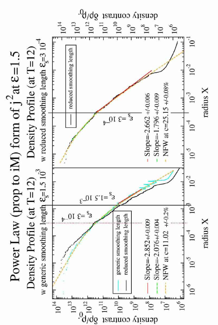
Figure 2: Smaller smoothing length $\epsilon_{s}$ test run: density profiles for critical values of the angular momentum near the end of the self-similar quasi-equilibrium phase in the shallow ($\epsilon=\frac{3}{2}=1.5$) initial density profiles case using the ‘power law’ form of angular momentum

The motivation in (Moore et al. (1999)) for proposing an alternate universal profile to the NFW profile is based on their observation of a resolution dependence of the inner slope. This resolution problem was also pointed out in the studies by (Jing & Suto (2000)). (Moore et al. (1999)) claim that their results show that the inner slope converges towards their proposed profile.

We have tested our results under changes in resolution using two different ‘smoothing’ lengths.

Similarly to the results of (Moore et al. (1999)), an increase in resolution in our model steepens the profile. This can be measured by the increase of the concentration factor c when the ‘smoothing’ length is reduced, as seen on Fig. 2. Nevertheless, contrary to (Moore et al. (1999)), the NFW profile is still the best fit, provided the appropriate change in concentration factor has been performed.

We interpret these results in terms of the centrifugal acceleration at a given radius between the two ‘smoothing’ lengths: thus its regularised expression in the model reads

$$a_{c}=\frac{j^{2}r}{(r^{2}+\epsilon_{s}^{2})^{2}}.$$

Taking its value at radius $r_{0}\ll 1$ with $r_{0}\in\left[\epsilon_{s_{2}};\epsilon_{s_{1}}\right]$, and considering the dominant terms, one can see that

$$\left.\begin{array}[]{cc}for\;\epsilon_{s_{1}}&a_{c_{1}}\propto j^{2}r_{0}\\ for\;\epsilon_{s_{2}}&a_{c_{2}}\propto\frac{j^{2}}{r_{0}^{3}}\end{array}\right\}\Rightarrow a_{c_{1}}=a_{c_{2}}r_{0}^{4},$$

which yields $a_{c_{2}}/a_{c_{1}}=1/r_{0}^{4}\gg 1\Rightarrow a_{c_{2}}\gg a_{c_{1}}.$ In other words, to diminish $\epsilon_{s}$ depletes particles from the centre.

Therefore resolution appears to fix the magnitude of the NFW profile’s concentration parameter c. Nevertheless, we have established that the addition of angular momentum to CDM haloes transforms the single power-law density profile into two slope NFW type profile.

4 Phase space structure of the dark matter halo

4.1 Virial ratio and phase space projection

We begin by considering the $r$-$v_{r}$ projection of phase space and the corresponding virial ratios, for comparison with the well-known radial results (HW (99)). These are shown in Figs. 3 and 4 for the SSAM and the PLAM respectively. In each figure the ‘shallow’ and ‘steep’ initial profiles are displayed, although these in fact show little difference in behaviour. In our simulations we used ‘equal mass modeling’ of the ‘shells’.

In (HW (99)), the shell modeling used smaller masses for inner shells than for outer shells in order to improve the dynamical mass resolution at the beginning of the infall. This allowed for the SSIM’s quasi-equilibrium self similar state to be achieved almost as soon as the core forms, to the detriment of an accurate phase space description that is our objective here. The use of constant mass shells leads to a relatively coarser mass resolution in the central part of the halo, which part corresponds to the set of shells that first forms the core, and so the quasi-equilibrium state is not achieved as gracefully. In fact this choice results in a poor modeling of the constant self-similar mass flux needed to maintain self-similarity during the accretion of innermost shells into the core. Each new shell acts almost as an overdensity perturbation to the previously established core and disturbs it from self-similar equilibrium until it is ‘digested’ (Le Delliou (2001)). Thus the equal mass modeling simulation requires an initial period of stabilization to reach the self-similar quasi-equilibrium. This period should be roughly the time to accrete the shell of the unequal mass modeling simulation that possesses the same mass as the constant mass used here. This conjecture was successfully tested.

A major physical difference with the radial SSIM appears during the transition from the self-similar equilibrium to a virialized isolated system, for which the virial ratio is unity. There is a visible smoothing compared with the radial SSIM’s sharp transition: instead of falling almost instantly from the self-similar value to unity when the last shell falls in, the presence of angular momentum produces instead a slow decrease from the self-similar value to that of the isolated system. This begins earlier than in the radial SSIM case (as measured by $T$) and finishes later.

The phase space projections (the lower panels of figures 3 and 4 display the phase space distribution of shells in the radius-radial velocity plane) reveal that there remains a stream of outer particles for which the angular momentum is so large that they will never fall into the core (their rotational kinetic energy makes them unbound). Indeed, since the initial angular momentum distribution for the particles is monotonically increasing with radius, and since the angular momentum is conserved exactly throughout the simulations including the initial radial ordering until shells reach the core; so near the end of the self-similar phase, the shells with increasingly large angular momentum are contributing to the mass flux. Given higher and higher angular momentum, there is a point at which angular momentum induces an inner turn around radius at the size of the self-similar core. Particles with smaller angular momentum will be able to enter the core but with a reduced radial velocity compared with the purely radial radial SSIM. This gradual extinction of the mass flux due to increasing particle angular momentum (velocity anisotropy) gradually shifts the system from its intermediate quasi-static phase to its final virialized phase.

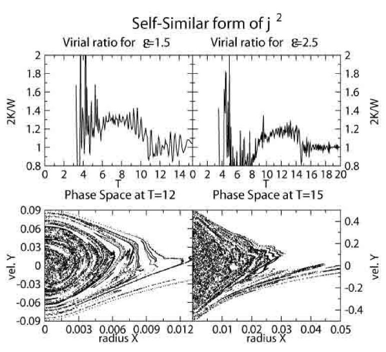
Figure 3: SSAM: virial ratios and phase space projections in the radius/radial velocity plane near the end of the self-similar quasi-equilibrium phase for critical values of the angular momentum in the shallow ($\epsilon=\frac{3}{2}=1.5$) and steep ($\epsilon=\frac{5}{2}=2.5$) initial density profiles cases

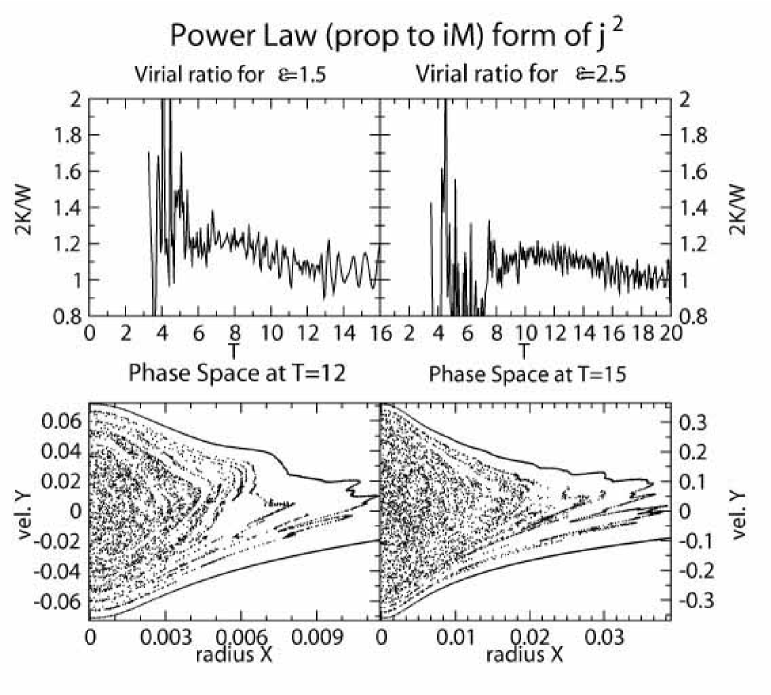
Figure 4: ‘Power law’ angular momentum (PLAM): virial ratios and phase space projections in the radius/radial velocity plane near the end of the self-similar quasi-equilibrium phase for critical values of the angular momentum in the shallow ($\epsilon=\frac{3}{2}=1.5$) and steep ($\epsilon=\frac{5}{2}=2.5$) initial density profiles cases

Comparing the phase space projections of the SSAM and the PLAM in Figs. 3 and 4 respectively we note that the SSAM seems less homogeneous. The exploration of the 3D phase space in Sect. 4.3 will confirm the impression that the SSAM is less relaxed in phase space during the accretion phase.

4.2 resolution effects

Considering the way resolution affects the virial ratio and $r$-$v_{r}$ projection of phase space, the previous remarks on the system’s relaxation can be extended.

The previous stabilisation delay for equal mass ‘shell’ modeling is increased when using the reduced ‘smoothing’ length. Here this period encompasses almost all of the self-similar phase (Fig. 5’s upper panels). Nevertheless, the right panel indicates that there still is an interval where the virial ratio is slowly decreasing from a higher value than 1.

We interpret this interval as due to the increase in the maximum acceleration felt by shells in the central parts of the halo: the scattering of shells is then much stronger, which makes it more difficult for the system to settle down. To minimise this inertial noise, the mass resolution should follow the ‘smoothing’ length reduction. We adopted an optimum balance between the mass, force and time resolutions found by trial and error.

It is remarkable that the noise in the virial ratio (Fig. 5) is diminished with the ‘smoothing’ length: if on one hand the equilibrium is achieved slower, it is on the other hand of a more stable final nature. Thus even if the mass flux resolution is not sufficient to account for the stabilisation delay, it still provides a good basis of understanding the relaxed system.

Adding to this picture, the phase space of the smaller $\epsilon_{s}$ simulation appears more relaxed than its larger $\epsilon_{s}$ counterpart; the relaxation region at the edges of the system restricts itself to the first outer stream and all traces of the phase space mixing sheets washes out (Fig. 5’s lower right and left panels). Such relaxation explains why the smaller $\epsilon_{s}$ simulation’s phase space is slightly wider in radial velocity and narrower in radius. This also shows in the more concentrated smaller $\epsilon_{s}$ NFW fit (Fig. 2).

In the light of N-body studies such as that of Knebe et al. (Knebe et al. (2000)), inaccuracy in the dynamics from two body scattering excludes ‘smoothing’ lengths much smaller than that used in our regular simulations, at given mass resolution. The mass resolution limitations on accuracy as well as the smoothing-length-time-step relation shed light on the low smoothing length cut off.

The nature of relaxation in the SSIM leads to the density profile being trustworthy even below its ‘smoothing’ length, but only a few times above its mass resolution characteristic length. This is caused by the fact that relaxation in the SSIM essentially occurs in the few dynamical times that particles are freshly incorporated into the self-similar core, mainly around the secondary turnaround radii, i.e. near the radial boundary of the core.

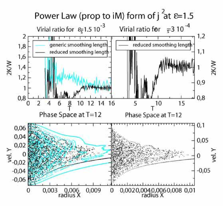
Figure 5: Smaller smoothing length $\epsilon_{s}$ test run: virial ratios and phase space projections in the radius/radial velocity plane near the end of the self-similar quasi-equilibrium phase for critical values of the angular momentum in the shallow ($\epsilon=\frac{3}{2}=1.5$) initial density profiles cases using the ‘power law’ form of angular momentum

All of the phase space maps presented are measured at T=12 which corresponds to a clear end of the self-similar infall phase and beginning of the isolated system virialised phase.

4.3 Three Dimensional Phase Space

This section explores the nature of the mass distribution in the radius-radial velocity-angular momentum phase space for systems with a shallow ($\epsilon=\frac{3}{2}$) initial density profile. The SSAM and PLAM models are both presented here for comparison purposes. All of these phase space maps are measured at T=12 which corresponds to a clear end of the self-similar infall phase and the beginning of the isolated system virialized phase. To get a complete sense of the topology of the winding and relaxation of the original Liouville stream of Hubble flow shells, we use tilted projections of the (X,Y,$j^{2}$) space. We recall that initially, with the power law distribution of angular momentum and the Hubble radial velocity, the particles lie on a curve in this phase space.

Figs. 6, denoted from top left to bottom right (a), (b) and (c), allow for a finer analysis of the final state: (a) shows a clear relaxation. The core appears to be rather smoothly populated in this projection. Fig. 6 (b) displays more clearly the outer phase mixing streams. The most striking fact that is made clear in Fig. 6 (c) is that the relaxed shells lie on a thin surface in phase space: this is a 2-dimensional sheet in the shape of a soaring bird, the neck and beak pointing toward large radius and angular momentum, while the high velocity wings spread progressively over higher and higher values of $j^{2}$. The accumulation of shells at low radius forms a flat basin.

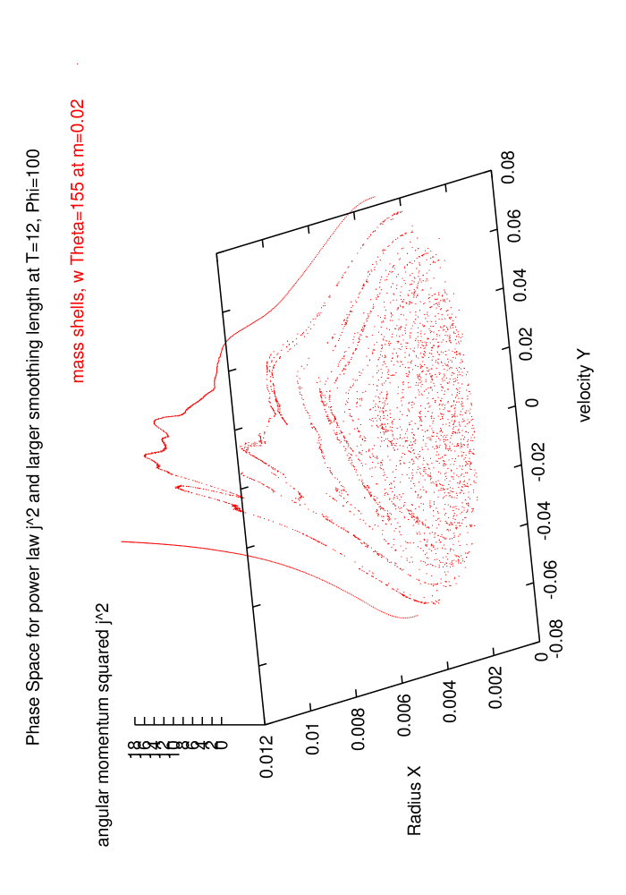
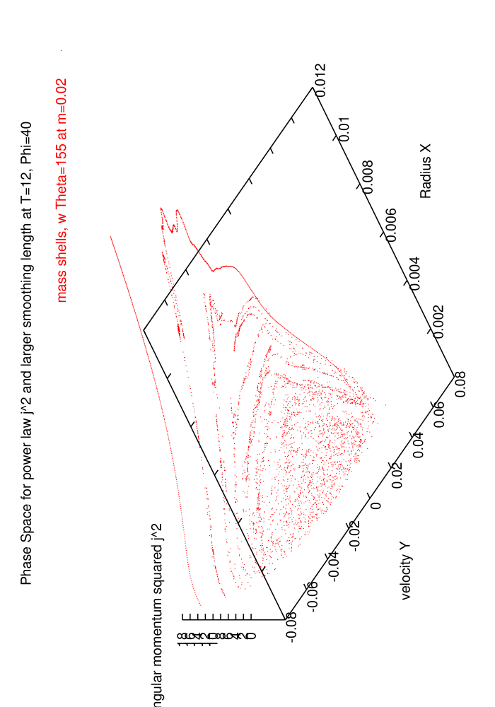
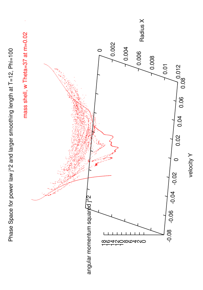
Figure 6: Phase space exploration using the ‘power law’ form of angular momentum near the end of the self-similar quasi-equilibrium phase (shallow initial density contrasts $\epsilon=\frac{3}{2}=1.5$ ). 3d views from top left to bottom: front view from underneath; side view from underneath; front view from above.

The phase space from the SSAM initial angular momentum distribution displays increased Liouville stream structure (and is therefore less relaxed) than for the power law case presented above. Fig. 7 reveals that the distribution of particles, although it peaks near the same surface as that found for the ‘power law’ initial angular momentum distribution in Fig. 6, is non-zero throughout a substantial region of phase space compared to the mean position. This is more pronounced for the SSAM despite the difference in scales used for the angular momentum in the two figures. Relaxation is clearly not as advanced in this case. It seems that the strict self-similarity before shell-crossing better segregates the shells in phase space. This recalls the importance of available phase space volume to relaxation pointed out by Tormen et al. (Tormen et al. (1997)), Teyssier et al. (Teyssier et al. (1997)) and Moutarde et al. (Moutarde et al. (1995)). The enhanced phase space volume per particle inhibits relaxation.

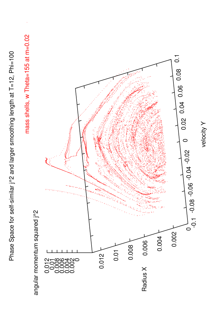
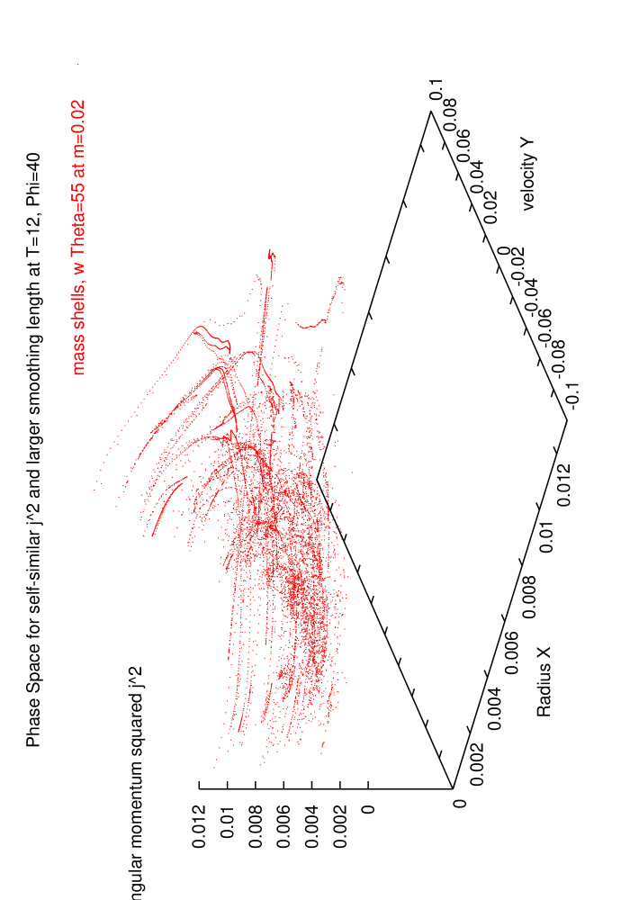
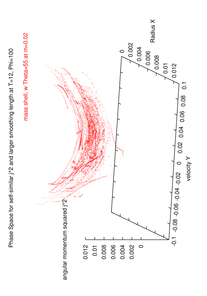
Figure 7: Phase space exploration using the self-similar form of angular momentum near the end of the self-similar quasi-equilibrium phase (shallow initial density contrasts $\epsilon=\frac{3}{2}=1.5$ ). 3d views from top left to bottom: front view from underneath; side view from underneath; front view from above.

5 Angular momentum and mass correlation?

The existence of the phase space surface found in the previous section implies correlations in the various projections. Recently one group has reported finding a universal angular momentum profile in N-body simulations in terms of a halo’s cumulative mass (Bullock et al. (2001)) according to

$$M(<j)=M_{v}m\leavevmode\nobreak\ j/(j_{0}+j),$$ (21)

where $m$ and $j_{0}$ are correlated characteristic scales and $M_{v}$ is the halo’s virialized mass. However, one should bear in mind that the profile given by Eq.(21) has been criticized by other authors (van den Bosch et al. (2002); Chen & Jing (2002)), who claim it results from the ommission of particles, carrying what they call negative angular momentum, and thus not to represent truly a halo angular momentum profile. In fact, their negative angular momentum stands for an angular momentum projected on the total vector of the halo which points oppositely to the total vector. In our approach one half of the particles carry, according to this definition, negative angular momentum since our total vector should be $\overrightarrow{0}$ by symmetry. Throughout we have only worked with the square of the particle angular momentum.

(Bullock et al. (2001)) also find a power law describing the correlation between angular momentum and radially cumulative mass ($j(M)\propto M^{s}$ where $M=M(<r)$ and $s=1.3\pm 0.3$). For this reason we consider these correlations in the two systems of the previous section in order to determine whether our choice of initial angular momentum is compatible with these simulations.

Dimensional analysis and the definition of the final density profile as $\rho\propto r^{-\mu}$ leads one to approximate the self-similar model’s relaxed state with power laws for the angular momentum ($j^{2}\propto r^{4-\mu}$) and for the mass profiles ($M\propto r^{3-\mu}$). Thus, $s$ can be predicted to be $s=\frac{4-\mu}{2(3-\mu)},$. In turn the SSIM gives the index $\mu$ as a function of the initial index $\epsilon$ as:

$$\mu=\left\{\begin{array}[]{ll}2&\epsilon\leq 2\\ \frac{3\epsilon}{1+\epsilon}&\epsilon>2\end{array}\right..$$

Although in the presence of enough angular momentum the radial SSIM results are expected to be altered, we are not really in that regime. Thus it is remarkable that the shallow initial density profile yields $s=1.$ The largest deviation in the SSIM from that value of $s$ is given for $\epsilon=3,$ since then $s=\frac{\epsilon+4}{6}=\frac{7}{6}\simeq 1.17,$ which is also within error from the (Bullock et al. (2001)) value.

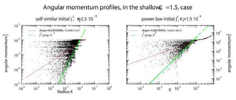
Figure 8: Two angular momentum profiles and their correlations

Empirically, the previous section’s phase space structure warns us that a correlation $M$ - $j^{2}$ may not be most readily found from a simple regression on all shells. Instead we might try to fit just the correlation from the projected mean surface about which the shells are distributed. The projection of phase space into the $j^{2}-X$ plane forms a caustic that appears to be a reasonable measure to compare with the predicted angular momentum profile. Fig. 8 illustrates the angular momentum profile correlations: the thin continuous lines are mere power law fits to all of the particles, and their values do not reflect the self-similar calculations. By contrast, a $j^{2}\propto X^{2}$ fit to the phase space caustic verifies the predictions for the shallow case. We have not investigated for this note the steep case but have no reason to believe the results would be different. Moreover, the density profiles show some steepening on the outer edges of the halo (Fig. 1), which translates into evidence for a flattening of the mass profile, hence of the mass-angular momentum profile as in Eq.(21).

These results are remarkable in that they rest on the idea that the dimensional angular momentum distribution used initially (17) also obtains in the ultimate halo. The same thing is true for the SSAM. Consequently the final correlation $j\propto r$ merely reflects the universality of the density profile in the intermediate ranges for the initially ‘flat’ density perturbation.

6 Summary

In this note we have studied the effects of particle angular momentum on the density profile and phase space structure of the final halo in the Self-Similar Infall Model (SSIM) for the formation of dark matter halos. We have used a simple shell code since the angular momentum averaged over each sphere is zero. We find the NFW profile to be an excellent fit to the density profile produced when an initial angular momentum distribution provided by simple dimensional arguments (PLAM) is assigned. This fit holds until the very central regions where extra flattening is expected on thermodynamic grounds (this flattening probably proceeds to a Gaussian with sufficient resolution (Henriksen & Le Delliou (2002))).

In addition we have shown that the initial line in phase space develops into a fairly well defined surface in phase space in the final halo. The ‘ridge’ or cusp of this surface when projected into angular momentum- position space is also predicted by the same dimensional argument. It seems then that some memory of the initial correlation between position and angular momentum is retained in the final object.

An alternate distribution of initial angular momentum (SSAM) that was designed to maintain strict self-similarity until shell crossing produces a less relaxed final phase space distribution (at the same dimensionless time) that is rather less precisely distributed on a 2D surface in the phase space. It is not able to reproduce the NFW density profile, perhaps because of the reduced relaxation (as displayed by the higher dimensionality in the final phase space).

The question as to whether the successful angular momentum distribution (PLAM) is actually established by tidal effects remains unanswered here. It essentially requires the rotational kinetic energy acquired by each halo particle to be a fixed fraction of the local halo gravitational potential. That the local gravitational potential should be an upper limit is clear, but it is not obvious why there should be a fixed fraction for all shells. One might assign $J^{2}$ as a random variable about some mean to see how sensitive the results are to a fixed value in the manner of (Sikivie et al. (1997)). However a coarse graining over the shells would tend to produce the same mean independent of $r$ and so we would expect a similar coarse-grained result to what we have found here. In fact Ryden & Gunn (Ryden & Gunn (1987)) do give the expected rms angular momentum distribution with mass for Gaussian random primordial perturbations. Their Fig. 10 suggests a linear relation in the range of masses that interests us here. This agrees approximately with our Eq. (20) when $\epsilon$ is close to 2 at moderate radii.

However although the results of the n-body simulations are usually given as spherical averages, it is not evident that this gives the same result as the strictly spherically symmetric calculation reported here. Nevertheless the agreement with the results of Bullock et al. (Bullock et al. (2001)) is encouraging in this sense , even though they may not contain all of the relevant physics(van den Bosch et al. (2002); Chen & Jing (2002)).

7 Acknowledgments

RNH acknowledges the support of an operating grant from the canadian Natural Sciences and Research Council. M LeD wishes to acknowledge the financial support of Queen’s University, Université Claude Bernard - Lyon 1 and Observatoire de Lyon, and to thank Stéphane Colombi for stimulating discussions.

References

- Aguilar & Merritt (1990) Aguilar, L.A., & Merritt, D., 1990, ApJ, 354, 33
- Bertschinger (1985) Bertschinger, E., 1985, ApJS, 58, 39
- van den Bosch et al. (2002) van den Bosch, F.C., Abel, T., Croft, R.A.C., Hernquist, L., & White, S., 2002, ApJ, 576, 21
- Bullock et al. (2001) Bullock, J.S., Dekel, A., Kolatt, T.S., Kravtsov, A.V., Klypin, A.A., Porciani, C., & Primack, J.R., 2001, ApJ,555, 240
- Carter & Henriksen (1991) Carter, B., & Henriksen, R.N., J.M.P.S., 1991, 32, 2580 (CH91)
- Chen & Jing (2002) Chen, D.N. & Jing, Y.P., 2002, MNRAS, 336, 55
- De Blok et al. (2001) De Blok, W.J.G., McGaugh, S.S., Bosma,A.,& Rubin V.C., 2001, ApJ 552, L23
- FG (84) Fillmore, J.A., & Goldreich, P., 1984, ApJ, 281, 1
- Ghigna et al. (1999) Ghigna, S., Moore, B., Governato, F., Lake, G., Quinn, T., & Stadel, J., 2000, ApJ, 544, 616,(1999, astro-ph/9910166)
- Henriksen (1989) Henriksen, R.N., 1989, MNRAS, 240, 917
- Henriksen & Le Delliou (2002) Henriksen, R.N., & Le Delliou, M., 2002, MNRAS, 331, 423
- HW (99) Henriksen, R.N., & Widrow, L.M., 1999, MNRAS, 302, 321 (HW99)
- Hoffman & Shaham (1985) Hoffman Y., & Shaham J., 1985, ApJ,297,16
- Hozumi,Burkert & Fujiwara (2000) Hozumi, S., Burkert, A., & Fujiwara T., 2000, MNRAS, 311, 377
- (15) Huss, A., Jain, B., & Steinmetz, M., 1999a, ApJ, 517, 64
- (16) Huss, A., Jain, B., & Steinmetz, M., 1999b, MNRAS, 308, 1011
- Jing (2000) Jing, Y.P., 2000, ApJ, 535, 30
- Jing & Suto (2000) Jing, Y.P., & Suto, Y., 2000, ApJ, 529, L69
- Jing & Suto (2002) Jing, Y.P., & Suto, Y., 2002, ApJ, 574, 538
- Knebe et al. (2000) Knebe, A. Kravtsov, A.V., Gottl ber, S., &Klypin, A.A., 2000, MNRAS, 317, 630
- Kravtsov et al. (1998) Kravtsov, A.V., Klypin, A.A., Bullock, J.S., & Primack, J.R., 1998, ApJ, 502, 48
- Le Delliou (2001) Le Delliou, Morgan, 2001, Ph.D. thesis, Queen’s Univ. at Kingston, Canada
- Lokas & Hoffman (2000) Lokas E. L.,& Hoffman Y., 2000, ApJ,542,L140
- Merrall (2003) Merrall, T.E.C., and Henriksen, R.N., 2003, ApJ, in press
- Moore (1994) Moore, B., 1994, Nature, 370, 629
- (26) Moore, B., Ghigna, S., Governato, F., Lake, G., Quinn, T., & Stadel, J., Proc. of 12th Potsdam Cosmology Workshop, Large Scale Structures: Tracks and Traces (Potsdam), eds. V. Mueller, S. Gottloeber, J.P. Muecket, & J. Wambsganss, World Scientific (1998) 37 and Proc. of Galactic Halos (U.C. Santa-Cruz), ed. D. Zaritsky, ASP Conference Series 136 (1998a) 426, (astro-ph/99711259)
- (27) Moore, B., Governato, F., Quinn, T., Stadel, J., & Lake, G., 1998b, ApJ, 499, 5
- Moore et al. (1999) Moore, B., Quinn, T., Governato, F., Stadel, J., & Lake, G., 1999, MNRAS, 310, 1147
- Moutarde et al. (1995) Moutarde, F., Alimi, J.-M., Bouchet, F.R., & Pellat, R., 1995, ApJ, 441, 10
- Nakano & Makino (1999) Nakano T., & Makino J., 1999, ApJ, 525,L77
- (31) Navarro, J.F., Frenk C. S., & White S.D.M., 1996, ApJ, 462, 563 (NFW)
- Peebles (1993) Peebles, P.J.E., 1993, Principles of Physical Cosmology, (Princeton: Princeton University Press)
- Ryden (1993) Ryden, B.S., 1993, ApJ, 418, 4
- Ryden & Gunn (1987) Ryden, B.S., & Gunn, J.E., 1987, ApJ, 318, 15
- Sikivie et al. (1997) Sikivie, P., Tkachev, I.I.,& Wang, Y., 1997, Phys.Rev.D, 56, 1863
- Stil (1999) Stil, J., 1999, Doctoral Thesis, Leiden Observatory
- (37) Subramanian, K., Cen, R., & Ostriker, J.P., 2000, ApJ, 538, 528, (1999a, astro-ph/9909279)
- (38) Subramanian, K., 2000, ApJ, 538, 517, (1999b, astro-ph/9909280)
- Syer & White (1998) Syer, D., & White, S.D.M., 1998, MNRAS, 293, 337
- Teyssier et al. (1997) Teyssier, R., Chièze, J.P., & Alimi, J.-M., 1997, ApJ, 480, 36
- Tittley & Couchman (2000) Tittley, E.R., & Couchman, H.M.P., 2000, MNRAS, 315, 834
- Tormen et al. (1997) Tormen, G., Bouchet, F.R., & White, S.D.M., 1997, MNRAS, 286, 865
- White & Zaritsky (1992) White, S.D.M., & Zaritsky, D., 1992, ApJ, 394, 1