The atoll source states of 4U 1608–52
Abstract
We have studied the atoll source 4U 1608–52 using a large data set obtained with the Rossi X-ray Timing Explorer. We find that the timing properties of 4U 1608–52 are almost exactly identical to those of the atoll sources 4U 0614+09 and 4U 1728–34 despite the fact that contrary to these sources 4U 1608–52 is a transient covering two orders of magnitude in luminosity. The frequencies of the variability components of these three sources follow a universal scheme when plotted versus the frequency of the upper kilohertz QPO, suggesting a very similar accretion flow configuration. If we plot the Z sources on this scheme only the lower kilohertz QPO and HBO follow identical relations. Using the mutual relations between the frequencies of the variability components we tested several models; the transition layer model, the sonic point beat frequency model, and the relativistic precession model. None of these models described the data satisfactory. Recently, it has been suggested that the atoll sources (among them 4U 1608–52) trace out similar three–branch patterns as the Z sources in the color–color diagram. We have studied the relation between the power spectral properties and the position of 4U 1608–52 in the color–color diagram and conclude that the timing behavior is not consistent with the idea that 4U 1608-52 traces out a three-branched Z shape in the color-color diagram along which the timing properties vary gradually, as Z sources do.
1 INTRODUCTION
Most of the neutron star low–mass X–ray binaries can be divided into two classes, Z and atoll sources, based on the correlated behavior of their timing properties at low frequencies ( Hz) and their X–ray spectral properties (Hasinger & van der Klis, 1989). Both classes show quasi-periodic oscillations (QPOs) with frequencies ranging from a few hundred Hz to more than 1000 Hz (kilohertz QPOs). The low–frequency part of the power spectra of both classes is usually dominated by a similar broad band–limited noise component, but it is unclear if these are physically the same component (Wijnands & van der Klis, 1999). In addition to the band–limited noise both classes show several quasi-periodic oscillations below 200 Hz. In the Z sources these are named after the branch of the Z track in the color–color diagram (see below) where they mostly occur: horizontal (HBOs), normal (NBOs) and flaring branch oscillations (FBOs). The HBO shows a sub– and a second harmonic at and times the frequency of the main peak, and sometimes a peak at times the frequency of the HBO (Jonker et al., 2002). Obviously, the most straightforward interpretation of this is that the sub HBO is the fundamental frequency, with second, third and fourth harmonics all observed (Jonker et al., 2002). Below 200 Hz the atoll sources show several Lorentzian components (see e.g. van Straaten et al., 2002). Note that these components are called Lorentzian and not QPO; this is because these features are sometimes too broad (FWHM centroid frequency/2) to be classified as a QPO. In the atoll sources all components become broader as their characteristic frequency decreases (Psaltis, Belloni & van der Klis, 1999; van Straaten et al., 2002). It has been suggested that the HBO in the Z and the low–frequency Lorentzian in the atoll sources are the same physical components (Ford & van der Klis, 1998; Psaltis et al., 1999; Wijnands & van der Klis, 1999).
The energy spectrum of neutron star low–mass X–ray binaries can be usefully parametrized through the use of color–color or color–intensity diagrams, where a color is the ratio of counts in two different energy bands. As the energy spectrum of a source changes, it moves through these diagrams. The timing properties of both the Z and the atoll sources depend on the position of the source in the color–color diagram. The Z sources move fast through the color–color diagram and draw up a Z track within hours to days (see e.g. GX 340+0; Jonker et al., 2000) whereas the typical atoll sources move slowly through the color–color diagram and draw up a C–shaped track within weeks to months (see e.g. 4U 1728–34; Di Salvo et al., 2001), although the “banana” part of the track, a curved branch to the bottom and right hand sides of the diagram, is traced out as fast as in the Z sources. The slow motion in the island part of the diagram, to the left hand and top sides, combined with observational windowing, tends to lead to the formation of isolated patches of data points, which is the origin of the term “island state” (Hasinger & van der Klis, 1989). Whereas the continuum power spectra of the banana state are dominated by a power law component at low frequencies with perhaps a weak band–limited noise component (which becomes stronger as the source approaches the island state), the island state power spectra are dominated by the band–limited noise. As the source moves away from the banana into the island state the count rate drops, the X–ray spectrum becomes harder and the band–limited noise becomes stronger while its characteristic frequency decreases. In the most extreme island states (4U 1608–52; Yoshida et al. 1993; Méndez et al. 1999; 4U 0614+09; Méndez et al. 1997; van Straaten et al. 2000; 4U 1728–34; Ford & van der Klis 1998; Di Salvo et al. 2001; 4U 1705–44; Langmeier, Hasinger & Trümper 1989; Berger & van der Klis 1998; Ford, van der Klis & Kaaret 1998; Aql X–1; Reig et al. 2000; KS 1731–260; Muno et al. 2000) the source is faint and hard and the band–limited noise is strong; this is the state in which neutron stars are most similar to BHCs in the low hard state (van der Klis, 1994a; Crary et al., 1996; Olive et al., 1998; Berger & van der Klis, 1998). Because of the low count rates and slow motion through the color–color diagram the precise properties of the extreme island state have been hard to ascertain, although observations of 4U 1608–52 with Tenma (Mitsuda et al., 1989) indicated the existence of an extended branch in this state that was traced out over an interval of weeks.
Recently, Muno, Remillard & Chakrabarty (2002a) and Gierlinski & Done (2002a) used large data sets from the Rossi X–ray Timing Explorer (RXTE) to study the color–color diagrams of several of the Z and atoll sources, which contain interesting additional information about, in particular, the nature of the extreme island state in the transient atoll sources 4U 1608–52, 4U 1705–44 and Aql X–1. They suggested that the atoll sources trace out similar three–branch patterns as the Z sources, with the extreme island state cast in the role of Z source horizontal branch. However, these authors did not address the timing properties of the sources they studied.
In this paper, we continue our work on the correlated X–ray spectral and timing behavior of Z and atoll sources using RXTE (Wijnands et al., 1996, 1997, 1998a, 1998b; Ford et al., 1998; Méndez et al., 1997, 1999; Méndez & van der Klis, 1999; Reig et al., 2000; Jonker et al., 2000, 2002; van Straaten et al., 2000, 2001; Di Salvo et al., 2001; Homan et al., 2002) with an analysis of 4U 1608–52. In these previous analyses, we have found strong correlations between the behavior of the timing features and the position of the source in the color–color diagram in both Z and atoll sources. 4U 1608–52 is a transient source that shows outbursts with a recurrence time varying between 80 days and several years (Lochner & Roussel–Dupré, 1994). low–frequency QPOs were discovered in the “island” state of 4U 1608–52 with the Ginga satellite (Yoshida et al., 1993) and kilohertz QPOs were discovered with RXTE (van Paradijs et al., 1996; Berger et al., 1996). The source was included in the samples studied by Muno et al. (2002a) and Gierlinski & Done (2002a) and was one of the sources that was reported to show Z–like behavior in the color–color diagram. By connecting the timing with the energy spectral properties we can test whether 4U 1608–52 indeed behaves as a Z source. If this is true one would expect the power spectral properties to change smoothly along the Z track, as is the case in the Z sources. We find that this is not the case. In §5 we also perform a more general comparison of frequencies observed in the Z and the atoll sources.
Parallel tracks in color–color and color–intensity diagrams were first observed in the Z sources (Hasinger et al., 1990; Kuulkers et al., 1994) and later also in the atoll sources 4U 1636–53 (Prins & van der Klis, 1997; Di Salvo, Méndez & van der Klis, 2003), 4U 1735-44 (Wijnands et al., 1998c) and 4U 0614+09 (van Straaten et al., 2000). Recently Muno et al. (2002a) reported further parallel tracks in the color–intensity diagrams of several atoll sources. The parallel–track phenomenon in the plot of lower kilohertz QPO frequency versus intensity was first observed in 4U 0614+09 (Ford et al., 1997) and 4U 1608–52 (Yu et al., 1997) and has since been observed in several more atoll sources (see e.g. Méndez, 2000). It has been suggested that the parallel tracks in the plot of intensity versus frequency of the lower kilohertz QPO and the parallel tracks in the color–intensity diagrams might be the same phenomena (van der Klis, 2000, 2001; Muno et al., 2002a). Van der Klis (2001) has proposed a possible explanation for this parallel track phenomenon in terms of a filtered response of part of the X–ray emission to changes in the mass accretion rate through the disk. The frequency versus intensity parallel–track phenomenon is particularly clear in 4U 1608–52 (Méndez et al., 1999). In §4 we investigate the relation between these frequency versus intensity parallel tracks and the parallel tracks in the color–intensity diagrams.
2 OBSERVATIONS AND DATA ANALYSIS
In this analysis we use all available public data from 1996 March 3 to 2000 May 24 from RXTE’s proportional counter array (PCA; for more instrument information see Zhang et al., 1993). The data are divided into observations that consist of one to several satellite orbits. We exclude data for which the angle of the source above the Earth limb is less than 10 degrees or for which the pointing offset is greater then 0.02 degrees. In our data set we found 7 type I X–ray bursts and we exclude those ( s before and s after the onset of each burst) from our analysis.
We use the 16–s time–resolution Standard 2 mode to calculate the colors. For each of the five PCA detectors (PCUs) we calculate a hard color, defined as the count rate in the energy band 9.716.0 keV divided by the rate in the energy band 6.09.7 keV, and a soft color, defined as the count rate in the energy band 3.56.0 keV divided by the rate in the energy band 2.03.5 keV. Per detector we also calculate the intensity, the count rate in the energy band 2.016.0 keV. To obtain the count rates in these exact energy ranges we interpolate linearly between count rates in the PCU channels. We calculate the colors and intensity for each time interval of 16 s. We subtract the background contribution in each band using the standard background model for the PCA version 2.1e.
In order to correct for the changes in effective area between the different gain epochs and for the gain drifts within those epochs as well as the differences in effective area between the PCUs themselves we used the method introduced by Kuulkers et al. (1994): for each PCU we calculate the colors of the Crab, which can be supposed to be constant in its colors, in the same manner as for 4U 1608–52. We then average the 16 s Crab colors and intensity per PCU for each day. In Figure 1 we can see the clear differences in the soft color trends of Crab between the five PCUs caused by the effects mentioned above. For each PCU we divide the 16 s color and intensity values obtained for 4U 1608–52 by the corresponding Crab values that are closest in time but within the same gain epoch. We then average the colors and intensity over all PCUs. If we multiply the soft color by 2.36, the hard color by 0.56 and the intensity by 2400 c/s/PCU we approximately recover the observed, uncorrected values for 4U 1608–52 (quoted values are averages of the Crab colors during the observations over all five PCUs). To improve statistics we rebin the 16 s color and intensity points to 256 s and exclude all data for which the resulting relative errors are larger than 5%. This led to a loss of about 40 ks of data at count rates below Crab. For most of these data neither timing nor colors were of sufficient quality to determine the source state. Starting May 12, 2000, the propane layer on PCU0, which functions as an anti–coincidence shield for charged particles, was lost. However, as all our data after May 12, 2000 ( ks) was excluded because the relative color errors were larger than 5% this was not a issue in our analysis.
For the Fourier timing analysis we use the 122s time–resolution Event and Single Bit modes and the 0.95s time–resolution Good Xenon modes. We only use data for which all energy channels are available. This led to a loss of about 9 ks of data in the lower banana state. In some observations there was data overflow in the timing modes due to excessive count rates from the source; we excluded those data. This led to a loss of about 27 ks of data at the highest intensity level (see also below). The power spectra were constructed using data segments of 256 s and 1/8192 s time bins such that the lowest available frequency is 1/256 Hz and the Nyquist frequency 4096 Hz; the normalization of Leahy et al. (1983) was used. To get a first impression of the timing properties at the different dates and positions in the color–color diagram, the power spectra were combined per observation. The resulting power spectra were then converted to squared fractional rms. We subtracted a constant Poisson noise level estimated between 2000 and 4000 Hz where neither noise nor QPOs are known to be present. As fit function we use the multi–Lorentzian function; a sum of Lorentzian components (Grove et al., 1994; Olive et al., 1998; Belloni, Psaltis & van der Klis, 2002) plus a power law to fit the VLFN (see van Straaten et al., 2002). We only include those Lorentzians in the fit whose significance based on the error in the power integrated from 0 to is above 3.0 . Two to five Lorentzian components were generally needed for a good fit. For the Lorentzian that is used to fit the band–limited noise we fixed the centroid frequency to zero. We plot the power spectra in the power times frequency representation (; e.g. Belloni et al., 1997; Nowak, 2000), where the power spectral density is multiplied by its Fourier frequency. For a multi–Lorentzian fit function this representation helps to visualize a characteristic frequency, , namely, the frequency where each Lorentzian component contributes most of its variance per logarithmic frequency interval: in the Lorentzian’s maximum occurs at (, where is the centroid and the HWHM of the Lorentzian; Belloni et al., 2002). We represent the Lorentzian relative width by defined as .
3 A TIMING TOUR THROUGH THE COLOR–COLOR DIAGRAM
In this section we try to get an idea of the timing properties of the source as it moves through the color–color diagram. We step through the data in chronological order and look at the timing properties (per observation, see §2) and the position of the source in the color–color diagram. In this way we select continuous time intervals for which the power spectrum and the position in the color–color diagram remain similar. For each continuous time interval we construct a representative power spectrum by adding up all observations within that interval. To get a first idea of the timing properties we made initial fits to the representative power spectra of the continuous time intervals using the multi–Lorentzian fit function described in §2. In most cases the power spectral features present could be directly identified with known components seen in other atoll sources by comparing with the power spectral features of 4U 0614+09 and 4U 1728–34 (using Figures 1, 2 and 3 of van Straaten et al., 2002). A more thorough fitting and description of the power spectral features will be presented in §3.4 where we obtain optimal statistics by constructing representative intervals for all our data by adding up the continuous time intervals that have similar positions in the color–color diagram and show similar power spectra.
The data on 4U 1608–52 can be usefully divided into 3 segments. The first segment ranges from 1996 March 3 to December 28 (the decay of the 1996 outburst, see Berger et al., 1996), the second segment from 1998 February 3 to September 29 (the 1998 outburst, see Méndez et al., 1998) and the third segment from 2000 March 6 to May 10 (persistent data). In practice most data were available for the second segment (the 1998 outburst) so we will present the results for the second segment first. These results can then serve as a template for the rest of the data.
3.1 Segment 2 (the 1998 outburst)
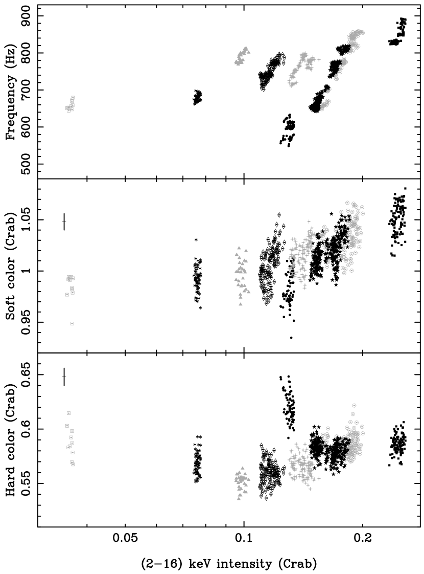
In Figure 2 we show as black points the lightcurve and color–color diagram for the second segment of the data (the 1998 outburst). The grey points in the lower frame represent the overall color–color diagram including all the data. Intensity and colors are normalized to the Crab (see §2). The numbers 9–17 (1–8 are reserved for the first segment of the lightcurve) indicate the continuous time intervals for which the power spectra and the position in the color–color diagram remain similar (see §3). The data for which no power spectra could be computed due to data overflow (see also §2) are indicated by the larger crosses at the peak of the outburst and in interval 9 of the color–color diagram. In Table 1 we present the duration of each interval, the time until the next interval and the 2–16 keV intensity during each interval. We identify several power spectral features and classify the continuous time intervals into color intervals A–J; these will be discussed in §3.4 where we put all information together. For the 1998 outburst we find 7 different classes, i.e., the source returns twice to similar positions in the color–color diagram where it displays similar power spectral shapes. Each class is marked with a different symbol in the color–color diagram of Figure 2.
For the 1998 outburst we confirm the result of Méndez et al. (1999) that the color–color diagram shows the classical atoll shape (see Hasinger & van der Klis, 1989). The characteristic frequencies of most of the power spectral components increase along the track starting at the open triangles and ending at the crosses in Figure 2 (for a more detailed discussion of the power spectral behavior with respect to the position in the color–color diagram, see §3.5).
3.2 Segment 1 (the decay of the 1996 outburst)
In Figure 3 we show as black points the lightcurve and color–color diagram for the first segment of the data (the decay of the 1996 outburst). The grey points represent the overall color–color diagram including all the data. The numbers 1–8 again indicate continuous time intervals for which the power spectra and the position in the color–color diagram remain similar. The symbols and entries in Table 1 are as described in §3.1.
We find one class additional to those observed during intervals 9–17. This class is composed of continuous time intervals 2, 4 and 6, fills up the region between the open diamonds and the filled stars in the color–color diagram, and is marked with open stars in Figure 3. Note further that part of the open diamonds here are in a slightly different position in the color–color diagram, at a higher hard color and a lower soft color, than where they were during the second segment of the lightcurve. This is accompanied by a lower intensity. If we sort the classes by characteristic frequency as measured in the power spectra, the characteristic frequencies change along an “–shaped” track in the color–color diagram (see also §3.5).
3.3 Segment 3
In the third segment of the data the source count rates were low and in most observations one or more detectors were switched off. This, together with the short durations of the observations (only s per observation) led to bad statistics. In most cases it was impossible to identify any power spectral features, therefore the classification for this segment of the data was solely done on position in the color–color diagram. If any power spectral features were detected they were always consistent with this color–based classification. As before, in Figure 4 black points represent the lightcurve and color–color diagram for the third segment of the data and grey points the overall color–color diagram. The numbers 18–30 now indicate continuous time intervals for which the position in the color–color diagram remained similar, and the symbols mark the classification, here based on the position in the color–color diagram only; entries in Table 1 are as described in §3.1. Note that the source is in the class marked with the crosses for only the second time during continuous time interval 21, but now at much lower intensity (0.03 Crab) than it was the first time in continuous time interval 9 (0.24–1.30 Crab) at the peak of the 1998 outburst.
3.4 The combined power spectra
To improve the statistics we average the power spectra in each of the 8 classes. In the class marked with the filled circles the lower kilohertz QPO is extremely narrow and varies in frequency over several hundreds of Hz. This leads to multiple peaks in the power spectrum. Therefore we split up this class into three parts depending on lower kilohertz QPO frequency; the first with the lower kilohertz QPO ranging from 540 to 640 Hz, the second with the lower kilohertz QPO ranging from 640 to 710 Hz and the third with the lower kilohertz QPO ranging from 710 to 900 Hz. A finer division would have compromised the statistics at low frequencies. The observations in this class where no lower (or upper) kilohertz QPO was detected were added based on position in the color–color diagram. In Figure 5 we show the resulting 10 intervals in the color–color diagram and in Figure 6 we show the corresponding hard color and soft color vs. intensity diagrams. Note that the data for which no power spectra could be computed due to data overflow (see §2 and 3.1) are not included in Figures 5 and 6. We mark the different classes in order of increasing characteristic frequencies from A to J. We use letters here to avoid confusion with the numbered continuous time intervals of §3.
We fit each interval with the multi–Lorentzian fit function described in §2. For the intervals where the kilohertz QPOs have sufficiently high frequencies not to interfere with the low–frequency features and vice versa, we fit the kilohertz QPOs between 500 and 2048 Hz and then fix the kilohertz QPO parameters when we fit the whole power spectra. This is for computational reasons only; the results are the same as those obtained with all parameters free. If the value of a Lorentzian becomes negative in the fit, we fix it to zero. No significantly negative Q’s occured. The fits have a /dof below 1.4 for intervals A–G. For interval H the /dof is high (5.43); this is caused by the motion of the lower kilohertz QPO from 710 to 900 Hz (see above). For intervals I and J the /dof are 2.5 (dof = 100) and 1.8 (dof = 97). This is caused by deviations of the VLFN from the power law used to fit it (see appendix A).
We now specify the terminology that we will use for the various power spectral components. Typical power spectral components observed for the atoll sources are described for the two sources 4U 0614+09 and 4U 1728–34 in van Straaten et al. (2002). As in Belloni et al. (2002) we call the upper kilohertz QPO Lu and its characteristic frequency . The lower kilohertz QPO has been linked to a broad bump at to Hz found in the low luminosity bursters 1E 1724–3045, GS 1826–24 and SLX 1735–269 (Belloni et al., 2002) and in the atoll source 4U 0614+09 at its lowest characteristic frequencies (van Straaten et al., 2002). Although we emphasize that this identification is very tentative (see §5.2.1) we will, as was done in Belloni et al. (2002), call both the lower kilohertz QPO and this 10–25 Hz bump (which do not occur simultaneously), Lℓ (characteristic frequency ). No standard terminology yet existed for the hectohertz Lorentzian (Ford & van der Klis, 1998); here we will call it LhHz (characteristic frequency ). The behavior of the band–limited noise and QPOs in the 0.1–50 Hz range in the atoll sources 4U 1728–34 and 4U 0614+09 is complex (see also Di Salvo et al., 2001; van Straaten et al., 2002), we describe it as a function of or position in the color–color diagram (see Figure 8). First, the characteristic frequency of the band–limited noise increases from to Hz. In this phase the band–limited noise is broad and usually fitted with a zero–centered Lorentzian or a broken power law. Then at Hz this noise component appears to “transform” into a narrow QPO (called very low–frequency Lorentzian in van Straaten et al., 2002) whose frequency smoothly continues to increase up to Hz, while what appears to be another band–limited noise component appears at lower characteristic frequencies. It is unclear exactly how these three components are related. Here, to remain true to the naming scheme of Belloni et al. (2002) we call the band–limited noise component that becomes a QPO as well as the QPO it becomes Lb (characteristic frequency ) and the “new” broad band–limited noise appearing at lower frequency Lb2 (characteristic frequency ), but please note the uncertainties in the interpretation underlying this nomenclature. Finally, in the banana branch of 4U 1728–34 and 4U 0614+09 (where usually no kilohertz QPOs are detected) a broad Lorentzian is also present at Hz for which it is unclear whether it is Lb, Lb2 or a new component; here we shall list it as Lb2. The atoll sources 4U 1728–34 and 4U 0614+09 both additionally show a Hz Lorentzian at frequencies above Lb, called the low–frequency Lorentzian by van Straaten et al. (2002). At high characteristic frequencies ( Hz) this Lorentzian appears as a narrow QPO. At low characteristic frequencies ( Hz) this Lorentzian is broad and can be identified with the component in the low luminosity bursters which Belloni et al. (2002) call Lh (’hump’). For this reason, we also call this low–frequency Lorentzian Lh (characteristic frequency ). In some observations the low luminosity bursters show a narrow low–frequency QPO (called LLF in Belloni et al., 2002) simultaneously with Lh. The of LLF is slightly lower than that of Lh. For 1E 1724–3045 the Lorentzian centroid frequencies of LLF and Lh coincided but this was not the case for GS 1826–24 (Belloni et al., 2002). LLF was not observed in 4U 1728–34 or 4U 0614+09 and we also do not detect it in 4U 1608–52.
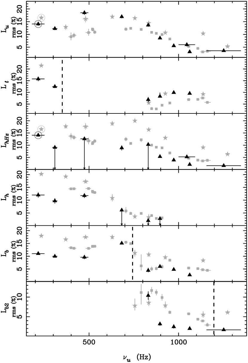
A detailed description of the behaviour of the power spectral components of 4U 1608–52 is given in appendix A. In Figure 7 we show the averaged power spectra and best fit functions of the intervals A–J. The fit parameters for the low–frequency part of the power–spectra are listed in Table 2, the fit parameters for the high–frequency part are listed in Table 3. We obtain 95% confidence upper limits for the fractional rms amplitude of LhHz in intervals B, C and E and of Lh in intervals B, C and E using , fixing to 0.2 and allowing to run between 100 and 200 Hz. For setting upper limits to Lh we fix to 1.5, 3.0 and 3.5 and let run between 22–32 Hz, 34–44 Hz and 42–50 Hz respectively (the values expected from the results for 4U 1728–34 and 4U 0614+09).
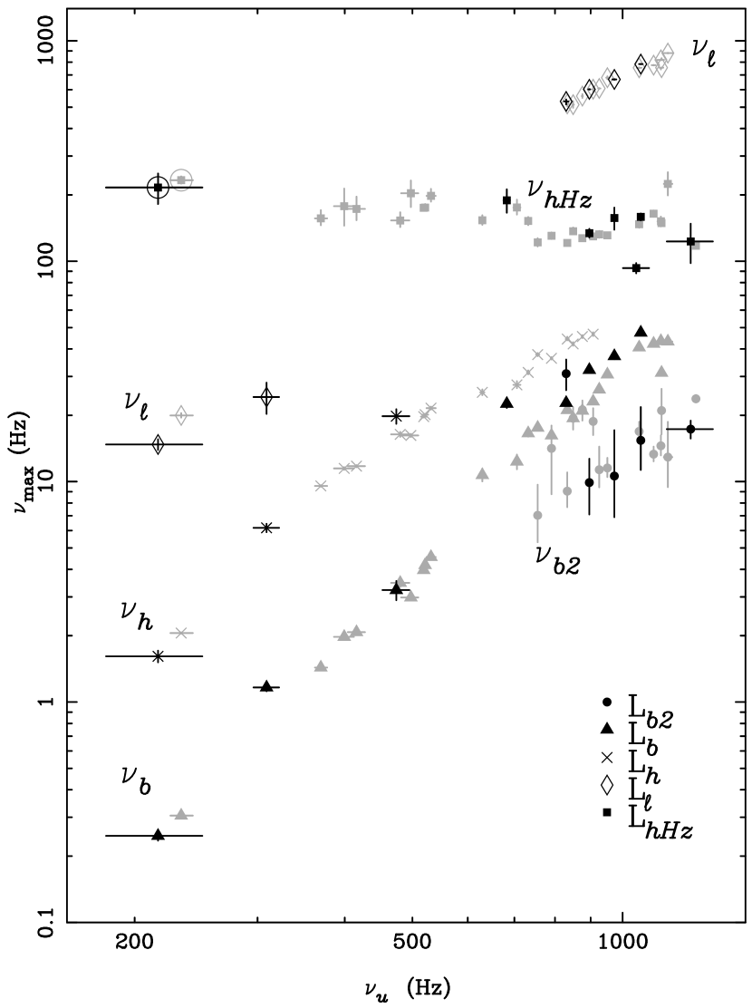
In Figure 8 we plot the characteristic frequencies of 4U 1608–52 versus , together with the results of van Straaten et al. (2002) for 4U 1728–34 and 4U 0614+09. The black points mark the results for 4U 1608–52, the grey points the results for 4U 1728–34 and 4U 0614+09. The different symbols indicate different power spectral components. The results for 4U 1608–52 mostly fall on the relations established for 4U 1728–34 and 4U 0614+09. Also the values of the various components versus are similar to those for 4U 1728–34 and 4U 0614+09. In Figure 9 we plot the rms fractional amplitude of all components versus . The general trends in this plot for 4U 1608–52 are similar to those of 4U 1728–34 and 4U 0614+09 (van Straaten et al., 2002), but there is an offset in rms between the relations for the three sources (Méndez, van der Klis & Ford, 2001). For the two kilohertz QPOs the rms fractional amplitudes in 4U 1608–52 are similar to those in 4U 0614+09 but larger than in 4U 1728–34 (Di Salvo et al., 2001). For all other features; LhHz, Lh, Lb, Lb2 and at low frequencies Lℓ the rms fractional amplitudes for 4U 0614+09 are the largest followed by 4U 1728–34 whereas the rms fractional amplitudes for 4U 1608–52 are the lowest. As we describe in appendix A in more detail, both the relations in Figures 8 and 9 as well as a direct comparison with the power spectra of 4U 1728–34 and 4U 0614+09 (Figures 1 and 2 in van Straaten et al., 2002) allow us to identify the power spectral components of 4U 1608–52 in the different intervals within the identification scheme described above.
3.5 How does 4U 1608–52 move through the color–color diagram?
Now that we have described and identified all power spectral components in 4U 1608–52, we can link the timing properties (Tables 2 and 3) to the position in the color–color diagram. We can also link the timing properties and X–ray spectral properties to the classical island and banana states described by Hasinger & van der Klis (1989). Intervals A–D are occurrences of the island state (strong broadband noise with low , no VLFN) in which intervals A–C can be classified as the extreme island state. The extreme island state shows Lb, Lh, Lℓ and Lu all at low characteristic frequencies. The power spectral components are all broad and strong. Interval E forms a transition between the island state and the lower banana, it still has relatively strong broad band noise but also shows a pair of narrow kilohertz QPOs that are typical for what Hasinger & van der Klis (1989) called the lower left banana state. So, intervals F–H are all lower left banana state. Here the VLFN appears, the kilohertz QPOs are double, Lb transforms from a band–limited noise component into a QPO and Lb2 appears (see also §3.4). Intervals I and most of interval J are also still in what Hasinger & van der Klis (1989) called the lower banana state based on their position in the color–color diagram; only the upper right part in the color–color diagram of interval J is in the upper banana state based on color–color position. The VLFN is strong and the broad band noise is weak in these intervals. Intervals I and J show Lu at the highest frequencies, Lb2, and a strong VLFN component. The characteristic frequencies increase in order A–J and form an “–shaped” track in the color–color diagram.
Recently, Muno et al. (2002a) and Gierlinski & Done (2002a) studied the color–color diagrams of several of the Z and atoll sources, including 4U 1608–52, and suggested that the atoll sources trace out similar three–branch patterns as the Z sources. We observe the same shape of the color–color diagram for 4U 1608–52 as Muno et al. (2002a) and Gierlinski & Done (2002a) did (Fig. 5). Interval C in Figure 5 represents a deviation from the classical atoll shape. According to the interpretation of Muno et al. (2002a) and Gierlinski & Done (2002a) the source would have to move in the Z–track order D–AB–C in Figure 5. Interval C would then correspond to the horizontal branch of the Z sources. We observe a transition from D to C and back to D with gaps of three days during the decay of the 1996 outburst (Fig. 3). We also observe a transition from E to C and back to E with gaps of only one day during the decay of the 1998 outburst (Fig. 2). The source is first in E for an interval of day during which the hard color increases by (so day-1), then there is a gap of 0.9 day after which the source appears in C with an increase in hard color of (if the source moved directly from E to C day-1). Then in C there is an interval of day where the hard color increases by ( day-1). So this is consistent with the source moving directly from E to C at approximately constant speed (probably through D) and not through A or B as required if 4U 1608–52 behaved as a Z source. In C there is a gap of day after which the source appears again in C but at a slightly () lower hard color. For an day interval the source stays in C while the hard color decreases by ( day-1). Then there is a gap of day and after that the source has returned to E with a hard color of less ( day-1). This is consistent with the source moving directly back from C to E, again at constant speed, and not through A or B. Transitions from and to states A and B had gaps of 7 and more days, so it is impossible to draw conclusions from these. The characteristic frequencies of the timing features decrease in the order D–C–B–A (appendix A). This is also not consistent with the idea that 4U 1608-52 behaves as a Z source, as in Z sources the characteristic frequencies of the timing features increase along the Z starting at the horizontal branch (i.e., this would predict frequencies decreasing in the order DBAC). One might say that 4U 1608–52 draws up an approximate “” shape in the color–color diagram along which the characteristic frequencies of the timing features change smoothly.
4 A DETAILED STUDY OF THE PARALLEL TRACK PHENOMENA
Parallel tracks in the intensity versus lower kilohertz QPO frequency in 4U 1608–52 were discovered by Yu et al. (1997), and extensively studied by Méndez et al. (1999) and Méndez et al. (2001). The hard color and soft color vs. intensity diagrams of 4U 1608–52 (see Fig. 6) and those of several other atoll sources also show narrow parallel tracks (Prins & van der Klis, 1997; Di Salvo et al., 2003; Muno et al., 2002a). Based on the appearance of the diagrams, it has been suggested that there is a relation between these two types of parallel tracks (van der Klis, 2000, 2001; Muno et al., 2002a).
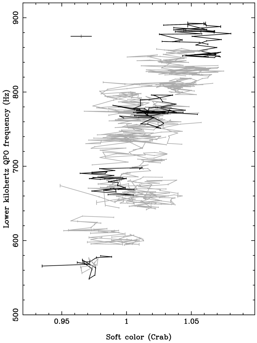
Based on our new analysis it is now possible to directly link the parallel tracks in the color intensity diagrams to those in the QPO frequency–intensity diagrams using the frequency of the lower kilohertz QPO as obtained by Méndez et al. (2001). Similarly to Méndez et al. (1999) and Méndez et al. (2001) we only include data for which both kilohertz QPOs are detected simultaneously and therefore the lower kilohertz QPO is identified unambiguously. We rebin our 16 s colors in such a way that they match the 64–448 s data intervals of Méndez et al. (2001). In Figure 10 we plot the frequency of the lower kilohertz QPO and the hard and soft color versus the 2.0–16.0 keV intensity. The alternating black/grey symbols represent the parallel tracks in the intensity versus the frequency diagram; the tracks contain data that are continuous in time, with only the s gaps due to Earth occultations. Note that the parallel track phenomenon in the lower kilohertz QPO frequency vs. intensity diagram is only observed in a small region of the color intensity diagrams (see Figure 6) where the lower kilohertz QPO is strong and narrow enough to be accurately traced on 64–448 s timescales.
With this analysis, we can investigate how the parallel tracks in the frequency vs. intensity diagram relate to those in the color intensity diagrams. Interestingly, it turns out that the frequency–intensity tracks can not, as previously thought, be identified with the narrow vertical tracks visible in the color intensity diagrams of Figures 6 and 10. Each of these latter tracks corresponds to a single satellite orbit. The parallel tracks in the frequency vs. intensity diagram are only identifiable as (rather fuzzy) tracks in the color intensity diagrams after several satellite orbits have elapsed and thus turn out to be composed of several of those narrow vertical tracks. The parallel tracks in the frequency versus intensity diagram could also identified in the hard color–intensity diagram of 4U 1636–53, where two banana tracks shifted by 20 % in intensity were observed in the hard color–intensity diagram (Di Salvo et al., 2003), and exactly the same 20 % shift was observed between the corresponding two parallel lines in the frequency versus intensity diagram. In 4U 1608–52 we do not observe complete banana tracks shifted in intensity as in 4U 1636–53. The drift in X–ray flux in 4U 1608–52 already occurs on timescales of several days (Méndez et al., 1999), too short for a complete track to form, where in 4U 1636–53 the source can stay on one track for several months (Di Salvo et al., 2003). These fast changes in intensity in 4U 1608–52 are due to its transient character, where 4U 1636–53 is a persistent source for which changes in intensity occur much more gradually. Note, that within each of the two parallel lines in the frequency versus intensity diagram of 4U 1636–53 there is no correlation observed between frequency and intensity.
The narrow vertical tracks in the color intensity diagrams are caused by variations in color that for the most part can be explained by the scatter due to counting statistics. The parallel tracks in the frequency versus intensity diagram, although composed of data covering several consecutive satellite orbits, already show up within individual orbits due to a short term correlation between the lower kilohertz QPO frequency and intensity in combination with small errors in these quantities but persist over several consecutive orbits. The correlation between colors and intensity (or kilohertz QPO frequency) in individual orbits is veiled by the limited counting statistics, so in the color intensity diagrams the parallel QPO tracks can only be identified on the longer timescales of several satellite orbits.
To further illustrate this point in Figure 11 we plot soft color versus the frequency of the lower kilohertz QPO; lines connect the points of individual satellite orbits, and for clarity four representative individual orbits are highlighted in black. On orbit time scales, the lower kilohertz QPO frequency and soft color seem uncorrelated due to the counting statistics errors on the color, whereas on a longer time scale a clear correlation emerges. We note that for some parallel tracks in Figure 6 there is a correlation between color and intensity on short timescales, especially in interval J. In those cases the counting statistics are better due to the higher count rates and thus the parallel track phenomenon in the color diagrams is more similar to that in the kilohertz QPO frequency versus intensity diagram (Muno et al., 2002a). However, in our interval J there is no timing feature present that is trackable on short timescales.
In conclusion we can now identify the parallel QPO tracks in the color intensity diagrams. Bad counting statistics that shows up in the form of the narrow nearly vertical parallel tracks in the color intensity diagrams cause the color correlation to be veiled on short timescales (less than hours) so in the color intensity diagrams the parallel QPO tracks can only be found for the longer timescales of several satellite orbits.
5 DISCUSSION
We have studied the color diagrams and the power spectral behavior of the atoll source 4U 1608–52. We found that the timing behavior of 4U 1608–52 is almost identical to that of the other atoll sources 4U 1728–34 and 4U 0614+09. If we plot the characteristic frequencies of the timing features versus the characteristic frequency of the upper kilohertz QPO, together with the results of van Straaten et al. (2002) for 4U 1728–34 and 4U 0614+09, the three sources follow the same relations (see Fig. 8). Also the behavior of the value is the same for the three sources. The general trends in rms fractional amplitude for 4U 1608–52 are also similar to those of 4U 1728–34 and 4U 0614+09, but there is an offset between the relations for the three sources (see Fig. 9). We connected the timing behavior with the position of the source in the color–color diagram and found that the timing behavior is not consistent with the idea that 4U 1608-52 traces out a three-branched Z shape in the color-color diagram along which the timing properties vary gradually as is the case in in Z sources. Instead, the power spectral properties change along an “–shaped” track. Finally, our measurements for the colors together with the precise measurements of lower kilohertz QPO frequency of Méndez et al. (2001) gave us an opportunity to link the parallel tracks in the intensity versus color diagrams with the parallel tracks in the intensity versus lower kilohertz QPO frequency diagrams. We found that the parallel tracks in the frequency versus intensity diagram can be found back in the color–intensity diagrams as fuzzy structures; they should not be confused with the narrow vertical parallel tracks visible in the intensity versus color diagrams which are mostly due to the errors in the colors.
5.1 Comparison with other sources; colors
The power spectral properties in 4U 1608–52 change along an “–shaped” track. The question now arises whether the “–shaped” track we find in the color–color diagram of 4U 1608–52 is universal for atoll sources. We can compare our results with those of Olive, Barret & Gierlinski (2003) who studied the X–ray color and timing properties of a well sampled state transition of 4U 1705–44 where the source moves from the lower banana to the extreme island state and back. This transition was also included in Muno et al. (2002a) who studied a larger dataset of 4U 1705–44. In the color–color diagram the source moves from the lower banana, to the left of the extreme island state as the count rate decreases. Then both the soft color and the count rate increase, whereas the hard color remains approximately constant, and the source traces out a horizontal track in the color–color diagram. Then, while the count rate continues to increase, the source moves back from the right of the extreme island state to the lower banana (Muno et al., 2002a; Barret & Olive, 2002; Olive et al., 2003). In the whole horizontal track the power spectra remained the same (Olive et al., 2003).
In this extreme island state 4U 1705–44 did not reach characteristic frequencies as low as those in interval A of 4U 1608–52 (it is very similar to interval B). If we look at the overall light and color curves of 4U 1705–44 presented in Muno et al. (2002a) we see that apart from the extreme island state just described, which took place in the forty days around MJD 51230, there is another extreme island state, with much sparser sampling, in which a higher hard color is reached. If we take a quick look at the timing of this MJD 51380 data we find that when the source reaches this higher hard color, the source shows a power spectrum very similar to that of interval A of 4U 1608–52. As for the MJD 51230 extreme island state, during this MJD 51380 extreme island state the count rate and the soft color increase simultaneously and in the color–color diagram another horizontal track is drawn up above the MJD 51230 one.
Returning now to 4U 1608–52 we note that in the state transition of 4U 1608–52 during the 1998 outburst (see Figure 2) we observe the same phenomenon of a horizontal track being traced out in the extreme island state. The source is in interval C (continuous time interval 12 in Fig. 2) for two observations, the first of which has a count rate about a factor two higher than the second. This higher count rate is accompanied by a 5 % higher soft color in the first observation. The power spectrum is the same in both observations. So, like the case of 4U 1705–44, the change in count rate is accompanied by a correlated change in soft color which traces out a small almost (the hard color changes slightly, see above) horizontal track in the color–color diagram (continuous time interval 12 in Fig. 2).
A possible explanation for this behavior of atoll sources in the extreme island state is the so–called “secular motion” in the color–color diagram. This phenomenon was first observed in Z sources, in which the Z–shaped track in the color–color and color–intensity diagrams is traced out within several hours up to a day. On longer timescales the whole Z track shifts both in soft color and count rate (e.g. Hasinger et al., 1990; Kuulkers et al., 1994; Jonker et al., 2000, 2002; Homan et al., 2002; Muno et al., 2002a). The timing properties remain mostly unaffected by these shifts and are primarily determined by the position along the Z track (e.g. Kuulkers et al., 1994; Jonker et al., 2000, 2002; Homan et al., 2002). The same phenomenon has been observed in the banana state of the atoll source 4U 1636–53 (Prins & van der Klis, 1997; Di Salvo et al., 2003). The horizontal tracks in the extreme island state of the atoll sources may be entirely caused by a secular motion, similar to that in the Z sources. Because the sources remain in one particular island state (similar timing properties and hard color) for a long time (weeks to months), the slow process of secular motion has time to draw up a horizontal branch. In this horizontal branch the timing remains similar, as is the case for Z source secular motion. As noted by Olive et al. (2003), this aspect of the behavior can be explained by the scenario that van der Klis (2001) proposed to explain the parallel track phenomenon in the intensity versus lower kilohertz QPO frequency diagram.
It seems that the Z shape in the color–color diagram of some of the atoll sources is caused by transitions between the banana and the extreme island states that occur at different soft color. Figure 12 provides a schematic of what in our interpretation occurs in these sources. Several different horizontally extended extreme island branches appear above each other in the color–color diagram at different hard color values. These are traced out at different epochs. To first order only the hard color determines the timing properties. Within each extreme island state the soft color changes in correlation with intensity. During state transitions the extreme island state is entered or left at a soft color value depending on intensity. A possible explanation for the fact that the timing remains similar while the intensity (and thus soft color) changes and that the state transitions can occur at different intensities (soft colors) is the scenario of van der Klis (2001) where the truncation radius of the disk, which determines the timing properties and therefore the state, is not set by the accretion rate through the disk but by the ratio of this accretion rate over its long–term average (c.f. Olive et al., 2003). So, if a source shows a state transition to an extreme island state at a minimum intensity which increases after that (as happened in the MJD 51230 state transition of 4U 1705–44 Muno et al., 2002a; Barret & Olive, 2002; Olive et al., 2003), the source will enter the extreme island state at a lower soft color and move to a higher soft color as the intensity increases. If a state transition to an extreme island state takes place during a decay after an outburst of a transient source, we would expect that after the extreme island state is entered at a particular soft color, the source then moves to a lower soft color as it fades (this and the reverse state transition from an extreme island to the banana state during the outburst rise were observed in Aql X–1, see Reig, van Straaten & van der Klis, 2003). In our interpretation, the shape we observe in the color–color diagram of 4U 1608–52 is caused by observations of the source in extreme island states at different intensities and therefore at different soft colors. Extreme island states A and B are observed at higher intensities than extreme island state C, causing C to have a lower soft color. Contrary to the case in 4U 1705–44 and Aql X–1 we do not observe a large change in soft color (or intensity) within each extreme island state and it is unclear whether this is because the source was not observed sufficiently long or dense enough in these extreme island states, or whether this is a property of 4U 1608–52.
5.2 Comparison with other sources; timing
5.2.1 Atoll sources, low luminosity bursters, and black hole candidates
The three atoll sources, 4U 1608–52, 4U 1608–52 and 4U 0614+09, we have studied up to now (van Straaten et al., 2002, this paper) show a similar and very distinct timing behaviour (Figures 8 and 9). 4U 1608–52 differs from 4U 0614+09 and 4U 1728–34 in that 4U 1608–52 is a transient source whose intensity changes by about 2 orders of magnitude where this is only about 1 order of magnitude for 4U 0614+09 and 4U 1728–34. Although 4U 1608–52 has a much larger range in intensity ( Crab in the 2.0–16.0 keV range) than 4U 0614+09 ( Crab), 4U 1608–52 and 4U 0614+09 show a similar range in characteristic frequencies for the different power spectral components. For 4U 1608–52 ranges from 216 to 1061 Hz (excluding intervals I and J for which the identification of is uncertain see appendix A). This range in is reached with a minimum intensity range of Crab (see Fig. 6). For 4U 0614+09 a similar range of 233 to 1067 Hz is reached with a minimum intensity range of Crab. So, both sources reach similar frequency ranges within a similar change in intensity. 4U 1728–34 has not yet shown a similar range in characteristic frequencies as 4U 0614+09 and 4U 1608–52 (until now Hz; Di Salvo et al., 2001; van Straaten et al., 2002). Also no 2.0–16.0 keV intensities were published for the intervals used in Di Salvo et al. (2001) and van Straaten et al. (2002).
There are also some differences in the timing behaviour; in particular in Lb when it appears as a QPO. As a function of , is slightly higher in 4U 1608–52 than in 4U 1728–34 and 4U 0614+09 but it covers the same range. The values for Lb here are similar for the three sources. The relation between and in Figure 8 has a turnover at 30 Hz in 4U 0614+09 (van Straaten et al., 2000); there might be a turnover at 45 Hz in 4U 1728–34, but in 4U 1608–52 no turnover has been observed. The plot of rms fractional amplitude of all components versus (Fig. 9) shows an offset between the relations for the three atoll sources 4U 1608–52, 4U 0614+09, and 4U 1728–34. This offset is different for the low–frequency features, LhHz, Lh, Lb, Lb2, and at low frequencies Lℓ, than for the two kilohertz QPOs (see also §3.4). It seems that there are two groups, one containing the high and the other the low–frequency features. The difference between the two groups might be due to geometrical effects. The different offsets in Figure 9 hint towards the Lorentzian at Hz, found in the lowest frequency states of 4U 1608–52 (interval A) and 4U 0614+09, being Lu (see appendix A), whereas it could have been identified as either Lu or LhHz based on its frequency (see appendix A). The identification of the Hz Lorentzian is important because the power spectra of 4U 1608–52 and 4U 0614+09 at the lowest inferred mass accretion rate closely resemble those of the low luminosity bursters 1E 1724–3045, GS 1826–24, and SLX 1735–269 (Belloni et al., 2002) and the millisecond X–ray pulsar SAX J1808.4-3658 (Wijnands & van der Klis, 1998). These sources all seem to be atoll sources that are only observed at low mass accretion rate. If the Hz Lorentzian is the upper kilohertz QPO then the high–frequency peaks in those sources are probably also upper kilohertz QPOs. Note that although in 4U 1608–52 Lh already becomes undetectable at Hz whereas this happens at Hz in 4U 1728–34 and 4U 0614+09, this is not a significant difference as the upper limits on the fractional rms of Lh in 4U 1608–52 are consistent with this component still being present at those frequencies.
The broad Lℓ component found in intervals A and B was previously found in 4U 1608–52 with Ginga by Yoshida et al. (1993) and has also been identified in the atoll source 4U 0614+09 (van Straaten et al., 2002). This component has also been found in the low–luminosity bursters 1E 1724–3045, GS 1826–24, and SLX 1735–269 (Belloni et al., 2002). The Lorentzian has been tentatively identified with the lower kilohertz QPO based on extrapolations of frequency–frequency relations (see Psaltis et al., 1999; Belloni et al., 2002; van Straaten et al., 2002). The rms fractional amplitude of the broad Lℓ is much higher than that of the lower kilohertz QPO (see Fig. 9), however, a similar increase in rms is visible in that Figure for Lu. But note that Lu is detected in all intervals where Lℓ is present as the lower kilohertz QPO in intervals H–E then dissapears in intervals D and C and only shows up again as the broad Lorentzian in intervals B and A.
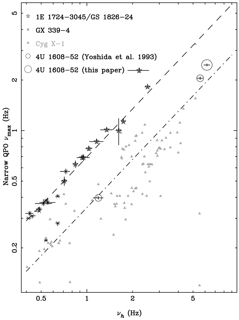
Interval B of 4U 1608–52 shows a narrow QPO with a characteristic frequency (2.458 Hz) between those of Lb and Lh. This QPO is probably the same as the one discovered in the island state of 4U 1608–52 by Yoshida et al. (1993): their power spectrum of the 1989 August 25–26 interval is very similar to our interval B, it has Lb with a characteristic frequency of Hz, Lh at Hz and a narrow QPO at Hz (see Figure 4 of Yoshida et al., 1993). The low–luminosity bursters 1E 1724–3045, GS 1826–24 (Belloni et al., 2002) as well as the BHCs GX 339–4 (Nowak, Wilms & Dove, 2002) and Cyg X–1 (Pottschmidt et al., 2002) also show narrow QPOs with a characteristic frequency between those of Lb and that of Lh. For 1E 1724–3045 the centroid frequency of the narrow QPO coincides with the centroid frequency of Lh, but for 4U 1608–52 this is not the case; here the centroid frequency of the narrow QPO ( Hz) is close to half the centroid frequency of Lh ( Hz). No similar narrow Lorentzians were fitted by van Straaten et al. (2002) for 4U 1728–34 or 4U 0614+09, but 4U 1728–34 does show narrow residuals between the characteristic frequency of Lb and that of Lh. In Figure 13 we plot versus the of these narrow QPOs. For Cyg X–1 many narrow QPOs were fitted by Pottschmidt et al. (2002); we only plot those QPOs that have a characteristic frequency between and . The points of the low–luminosity bursters and most of those of GX 339–4 line up in Figure 13. These QPOs were all labeled as LLF by Belloni et al. (2002). The two points of GX 339–4 that deviate from the line are from two observations where GX 339–4 showed two simultaneous QPOs; the highest frequency QPO falls on the relation in Figure 13 while the lowest frequency QPO falls below it. If we fit the points of the low–luminosity bursters and GX 339–4 with a power law our result as well as those of Yoshida et al. (1993) for 4U 1608–52 fall below this relation. So we can not identify this narrow QPO in 4U 1608–52 with LLF. In the two observations where GX 339–4 showed two narrow simultaneous QPOs, the characteristic frequencies of the lowest frequency QPO as well as the results for Cyg X–1 also fall well below the power law. It might be that these QPOs and those of 4U 1608–52 are related. These points fall close to a line that indicates half the low–luminosity burster relation which is also plotted in Figure 13. Note that if we use centroid frequency instead of the relations in Figure 13 worsen.
5.2.2 Z sources
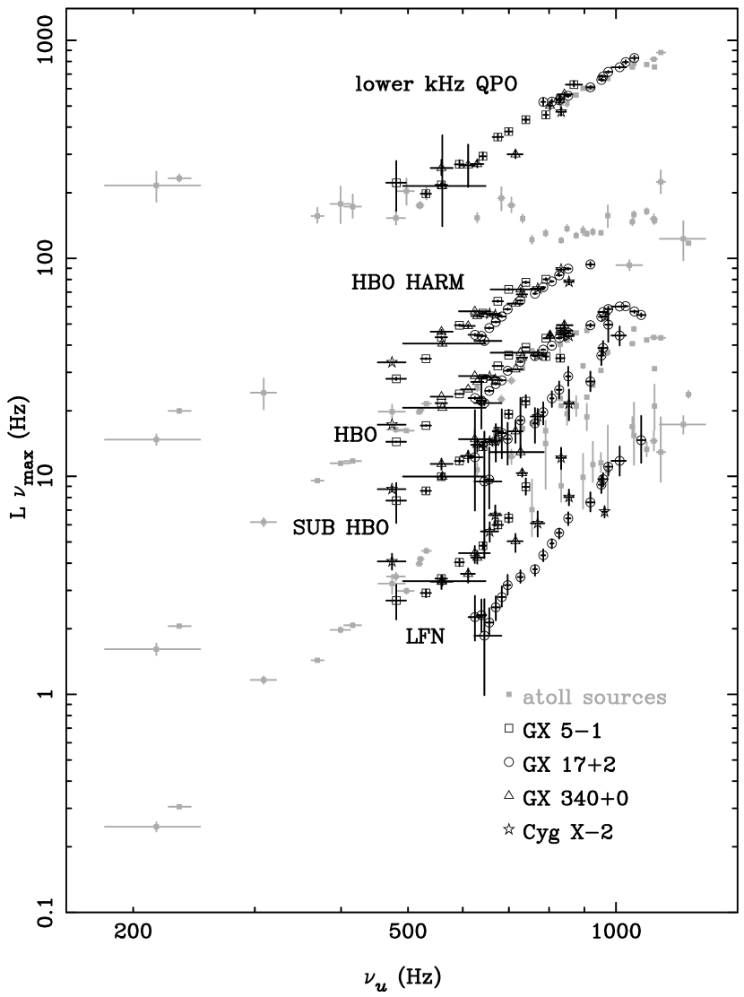
In addition to comparing the color–color diagram tracks and the associated power spectra, we can also compare the timing properties of Z sources with those of atoll sources by making similar plots of of the different power spectral components versus as we did for the atoll sources 4U 1608–52, 4U 0614+09 and, 4U 1728–34 in Figure 8. In Figure 14 we do this for the Z sources GX 5-1 (Jonker et al., 2002), GX 340+0 (Jonker et al., 2000), GX 17+2 (Homan et al., 2002) and Cyg X–2 (Kuznetsov, 2002). We include the lower kilohertz QPO, the Low–Frequency Noise (LFN), the Horizontal Branch Oscillations (HBO), and the harmonic and sub–harmonic of the HBO, and plot these versus . The grey symbols are the results of the atoll sources also displayed in Figure 8, the black symbols represent the Z sources. Note that the broad–band noise in these Z sources was not fitted with a zero–centered Lorentzian but with a cutoff power law, , for GX 5-1, GX 340+0, and GX 17+2 and with a smooth broken power law, , for Cyg X–2. This leads to expressions for , defined as the frequency of maximum power density in , of for the cutoff power law, and for the smooth broken power law.
From Figure 14 we confirm the identification of the HBO in the Z sources with Lh in the atoll sources made by Psaltis et al. (1999). However, the suggestions that either the LFN (van der Klis, 1994b; Jonker et al., 2000) or the sub–HBO (Wijnands & van der Klis, 1999; Jonker et al., 2000) in the Z sources might be similar to the classical broad–band noise in the island state of the atoll sources seems not to be supported by the relation of the characteristic frequencies of these components with . At Hz the band–limited noise component in the Lb–Lu relation is replaced by a QPO (see §3.4) and the band–limited noise component Lb2 appears and follows a new relation with . The LFN points fall below the Lb—Lu relation but seem to line up with Lb2. The sub–HBO points fall above the Lb—Lu relation until Hz where the QPO takes over from the band–limited noise component (see above).
Based on this comparison of frequencies, the LFN might still be associated with Lb2 and the sub–HBO might be related with Lb when it is a QPO, although for 4U 0614+09 and 4U 1728–34 no harmonic relation was present between Lh and Lb when it is a QPO (van Straaten et al., 2002). Note also that the LFN in GX 17+2 follows a different relation compared to that in the other Z sources. Other differences between GX 17+2 and the other Z sources in Figure 14 are that the LFN in GX 17+2 is peaked, the harmonic of the HBO is relatively strong and it shows a flaring branch oscillation (FBO) whereas the other sources show a flat LFN, a relatively weak harmonic of the HBO and no FBO (Jonker et al., 2002). We note that none of these differences with the other Z sources serve to make GX 17+2 more similar to the other atoll sources.
5.2.3 Summary
The results presented in sections 3.4, appendix A, and this section show that the low–frequency part of the power spectra of both the atoll and the Z sources behaves in a very complex manner. For the atoll sources many different Lorentzian components appear, disappear or change from broad Lorentzians into narrow QPOs. Although this behavior is complex, the power spectral components of the three atoll sources for which we have performed a multi–Lorentzian timing study show remarkable similarities. By using frequency vs. frequency plots such as the one in Figure 8, and by comparing the power spectra of different sources directly with each other it is possible to identify all these components within a single classification. We do this here for 4U 1608–52 (section 3.4). Note however, that sometimes additional narrow features become significant in the power spectra (see 5.2.1). As another example, a recent RXTE observation of 4U 1608–52 during an outburst in 2001, shows a power spectrum (Figure 15) very similar to that of interval B (Fig. 7), except that instead of the broad peak at Hz, a narrow () QPO with an rms fractional amplitude of appears at 30 Hz. Also several, marginally significant, features are visible between 2 and 5 Hz.
If we compare the low–frequency features of the atoll sources with those found in the Z sources, in a frequency vs. frequency plot we see that only the HBO of the Z sources can be unambiguously identified with the Lh of the atoll sources. The frequency vs. relations of the other low–frequency features partly overlap in Figure 8 but are not identical, and the relation of the characteristic frequency of the LFN with is not even the same for all Z sources. It appears that for some components the frequency vs. relations are not universal. There might be small physical differences between the atoll sources and Z sources (and within the Z sources themselves) that affect these relations. So, either these features are different phenomena in different types of sources, or something else (e.g. neutron star mass, magnetic field strength) affects the relations. If this is so, this hidden parameter does not change much from source to source, or the relations do not depend strongly on this parameter as the relations are similar, as the relations are very similar within each source type.
5.3 QPO models
Three different characteristic frequencies can be used to test the frequency relations predicted by the several QPO models; , and . is the frequency at which a Lorentzian contributes most of its variance per log frequency (Belloni et al., 2002) and is the one used in this paper. is the centroid frequency of the Lorentzian and can be obtained from our fit parameters and as . According to Titarchuk (2002) the of the Lorentzian is shifted with respect to the eigenfrequency of the oscillation due to damping. This shift depends on the damping rate which can be estimated from the width of the Lorentzian (Titarchuk, 2002). We can calculate this eigenfrequency, , from and as . In this section we use our fit parameter unless stated otherwise.
The transition layer model (TLM Osherovich & Titarchuk, 1999; Titarchuk & Osherovich, 1999) associates the lower kilohertz QPO with the Keplerian frequency of the inner disk edge (). Between the neutron star and the Keplerian disk a transition layer is present. In the TLM the upper kilohertz QPO is produced by radial oscillations of a blob thrown out of the transition layer into a magnetosphere. This radial eigenmode or hybrid frequency () relates to as , where is the rotational frequency of the star’s magnetosphere near the equatorial plane. This implies that should always exceed . For 4U 1608–52 Osherovich & Titarchuk (1999) found that is always larger than 300 Hz and thus Hz should apply. For 4U 1608–52 we find that when there is a pair of kilohertz QPOs present (intervals E–H) the upper kilohertz QPO frequency ranges from 830 to 1062 Hz. But the 200–682 Hz single kilohertz QPO of intervals A–D, which we identify as the upper kilohertz QPO based on frequency–color (Méndez et al., 1999; van Straaten et al., 2000; Di Salvo et al., 2001), frequency–frequency (Fig. 8) and rms–frequency (see Méndez et al., 2001, and Fig. 9) correlations, fall well below the 600 Hz predicted by the TLM model. Note that neither the use of , nor , shifts these frequencies above the 600 Hz limit. If these single kilohertz QPOs were not the upper, but the lower kilohertz QPOs, this would lead to the unlikely scenario that the presence of an upper kilohertz QPO would lead to a completely different power spectrum for a similar lower kilohertz QPO frequency (compare, e.g., C with E or D with G in Fig. 7).
The vs. relation for neutron stars and BHCs (see Psaltis et al. 1999 for the relation in the representation, and Belloni et al. 2002 for the relation in the representation) was recently extended towards lower frequencies by including 17 white dwarf sources (see Mauche, 2002; Warner & Woudt, 2003, and references therein). The points of 4U 0614+09, 4U 1728–34, and 4U 1608–52 fall on the vs. relation; only the point from interval B of 4U 1608–52 deviates. The vs. relation can be fitted with a power law with an index close to 1 (Psaltis et al., 1999; Mauche, 2002). The TLM explains this by assuming that is the Keplerian frequency of the inner disk (see above), and represents the frequency of magnetoacoustic oscillations, , in the disk transition layer. The relation between and is then a result of a global relation between of the transition layer and at the adjustment radius (Titarchuk & Wood, 2002). For each individual source the TLM predicts an index for the vs. relation that is steeper than one and should be studied separately (Titarchuk, Bradshaw & Wood, 2001). Note, however, that the atoll sources cover a large range of the vs. relation, as there are points around Hz and around Hz. While 4U 1608–52 only contributes points around Hz and 4U 1728–34 only around Hz, 4U 0614+09 contributes both. This suggests that the Psaltis et al. (1999) relation is not just a global relation between different sources as suggested by Titarchuk & Wood (2002) but can also be found within individual sources. Note also that although the TLM explains the Psaltis et al. (1999) relation as above in Titarchuk & Wood (2002), the HBOs of the Z sources, which are part of Psaltis et al. (1999) relation, are explained differently, namely as the vertical eigenmode of a blob rotating with a Keplerian frequency thrown into the magnetosphere (see above) in other TLM papers (e.g. Titarchuk, 2002).
In the sonic point beat frequency model (SPBFM; Miller, Lamb & Psaltis, 1998) the upper kilohertz QPO represents the Keplerian frequency at the inner disk edge. The lower kilohertz QPO then arises from a beat of the Keplerian frequency at the inner disk edge with the neutron star spin frequency. This led to an early prediction that , the frequency difference between the upper and the lower kilohertz QPO, is equal to the spin frequency and should therefore be constant. Observations of several sources, among which 4U 1728–34 (Méndez & van der Klis, 1999) and 4U 1608–52 (Méndez et al., 1998), showed a significant decrease in when the upper kilohertz QPO frequency increased. Further refinements of the SPBFM by Lamb & Miller (2001) could explain this decrease in . Neither the use of nor instead of makes constant. Note that our measurements of the high–frequency kilohertz QPOs ( Hz) are not the best to use here as the addition of a lot of data leads to an artificial broadening of the Lorentzian (see §3.4). Therefore here we used the precise measurements of these high–frequency kilohertz QPOs made by Méndez & van der Klis (1999) for 4U 1728–34 and by Méndez et al. (1998) for 4U 1608–52 to calculate and . For both sources increases by less than 1.5 % if is used instead of and by less than 3.1 % if is used instead of . Note that, just as for the TLM, the low frequencies we find for the upper kilohertz QPO (see above) are a problem for the SPBFM. In the SPBFM the lower bound on the upper kilohertz QPO frequency is set by the Keplerian frequency at the maximal radius where the radiation coming from the neutron star surface can still remove sufficient angular momentum from the gas in the disk so that it falls supersonically to the neutron star surface (Miller et al., 1998). This radius is about , where is the radius of the marginally stable orbit. So, to reach Hz the mass of the neutron star has to exceed .
The relativistic precession model (RPM; Stella & Vietri, 1998, 1999) assumes that the upper kilohertz QPO represents the Keplerian frequency of the inner disk. The lower kilohertz QPO frequency represents the periastron precession frequency of the accretion disk, which is assumed to contain slightly elliptical orbits. This leads to the prediction that the frequency difference () between the two kilohertz QPOs decreases both at low and high kilohertz QPO frequencies (see Figure 1 of Stella & Vietri, 1999). If the broad Lℓ at low frequencies (intervals A and B of 4U 1608–52 and interval 1 of 4U 0614+09 in van Straaten et al., 2002) is the lower kilohertz QPO (but see §5.2.1), then this predicted decrease in at low kilohertz QPO frequencies is observed in 4U 0614+09 and 4U 1608–52. Note that the point of interval B of 4U 1608–52 falls above the curves of Figure 1 in Stella & Vietri (1999) by . More complicated modelling within the framework of the RPM as is done for Sco X–1 in Stella & Vietri (1999) is beyond the scopes of this paper.
The RPM also predicts a low–frequency QPO at the Lense–Thirring precession frequency of Hz (Stella & Vietri, 1998), where is the moment of inertia in units of g cm2, is the mass of the neutron star in , and is the neutron star spin frequency. We searched our data for a power law with an index of 2 as predicted by the RPM by fitting the frequency vs. relations for the low frequency features (Fig. 8) for the three sources 4U 1728–34, 4U 0614+09 and 4U 1608–52 with power laws. We used , , and for the characteristic frequencies (see above). We find that the vs. relation has an index that is the closest to the 2 predicted by the RPM. If we use or for the frequency the relations clearly deviate from a power law. The points fall below the fitted power law at low and high frequencies and above at intermediate frequencies, leading to very large /dof of 4605/21 () and 7179/21 (). If we use for the frequency we find that the vs. relation can be described by a power law of the form (see Figure 16). The /dof of this fit is still high (373/20) but this is not due to systematic deviations from a power law. The averaged relative scatter around the fitted power law is only 6 % on the axis and only 3 % on the axis. The high /dof is probably a result of not including any systematic errors when determining the errors of the power spectral fit parameters (see Ford & van der Klis, 1998). Note, that if we use for the frequency we exclude those points that have (from fits with a zero–centered Lorentzian). The result that the vs. relation can be described by a power law with an index close to 2 was found previously for a more limited frequency range ( Hz) in 4U 1728–34 (index 2.11; Ford & van der Klis, 1998) and 4U 0614+09 (index 2.46; van Straaten et al., 2000). It is remarkable that now that we have extended the vs. relation towards Hz, the relation can still be described by a power law and that the power law index is found to be even closer to 2. We can get an indication of the spin frequency by looking at the burst oscillation frequency which is 363 Hz for 4U 1728–34 (Strohmayer et al., 1996) and 620 Hz for 4U 1608–52 (Muno et al., 2002b). If these two frequencies are the spin frequency of the neutron star in each case (the most likely scenario, see Chakrabarty et al., 2003), then it is difficult to understand why the vs. relations of these sources coincide. If we assume that we see the spin frequency in 4U 1728–34 and twice the spin frequency in 4U 1608–52, we find an average spin frequency of about 335 Hz for these sources. For the representation fit, this leads to which is too large for proposed equations of state (the acceptable range is ; Stella & Vietri, 1998). If we assume that we see the spin frequency in 4U 1608–52 and half the spin frequency in 4U 1728–34, the average spin frequency is about 670 Hz for these sources. This leads to which is acceptable.
5.4 The energy spectrum of 4U 1608–52
Recently, Gierlinski & Done (2002b) studied the X–ray energy spectra of 4U 1608–52 as a function of position in the color–color diagram. They find that, similar to other atoll sources, the spectra of the island state (our intervals A, B and C) of 4U 1608–52 are dominated by a hard power law spectrum. There is also a soft component present which in their view is probably due to the neutron star surface rather than the accretion disk. The banana state (our intervals E–J) spectrum is soft and it is uncertain whether the soft component is due to the neutron star surface or the disk. To explain the spectral behavior of 4U 1608–52 Gierlinski & Done (2002b) use a scenario where in the island state the disk is far from the surface of the neutron star. The large radius of the inner disk prevents the disk from being observed directly in the PCA spectra. In the island/banana state transition the inner accretion flow, which was geometrically thick and optically thin in the island state, collapses into a geometrically thin and optically thick disk. The inner edge of the disk is now close to the neutron star, and it is observed as the soft component and increases the soft color. From the DISKBB model, Gierlinski & Done (2002b) estimate an inner disk radius in the banana state of km. The inner accretion flow becomes more optically thick lowering the hard color. We can compare this scenario with the results of our timing study. If we assume that represents the Keplerian frequency at the inner disk edge (e.g. Miller et al., 1998) we find, assuming a neutron star mass of 1.4 M⊙ (for a different neutron mass the results change by a factor (M, which is 1.2 for a 2.4 M⊙ neutron star), that the inner disk terminates at km for the island state (intervals A, B and C). For the banana state (intervals E–J) we find an inner disk radius of km and decreasing towards higher soft color. Indeed we find that the inner disk radius is closer to the neutron star in the banana than in the island state, but the values in both the banana and the island state are close to the km estimated by Gierlinski & Done (2002b) for the banana state. So, the difference in radius between island and banana state seems too small to make the disk disappear from the PCA spectrum in the island state as proposed in the scenario of Gierlinski & Done (2002b) described above. If we assume that instead of , represents the Keplerian frequency at the inner disk edge (e.g. Titarchuk & Osherovich, 1999), this would lead to much larger differences in inner disk radius between the island ( km) and the banana state ( km), so this interpretation could be consistent with the Gierlinski & Done (2002b) scenario. The identification of as the Keplerian frequency at the inner disk edge is also suggested by the recently proposed extension of the PBK relation (Psaltis et al., 1999; Belloni et al., 2002) towards lower frequencies by including 17 white dwarf sources (see Warner & Woudt, 2003, and references therein). For the white dwarf sources a QPO is plotted versus the dwarf nova oscillation, DNO, the DNOs are thought to occur at the Keplerian frequency of the inner disk edge (Warner & Woudt, 2002, and references therein).
The behavior in the soft color vs. intensity diagram of 4U 1608–52 and 4U 1705–44 in their extreme island states can also be explained within the scenario of Gierlinski & Done (2002b). Let us assume that represents the Keplerian frequency of the inner disk edge. In the extreme island states the disk is far out at 200 km and can not be seen in the PCA energy spectrum (see above), the soft color should therefore only depend on the spectral properties of the neutron star. If we look at the extreme island states A and B of 4U 1608–52 and 4U 1705–44 in the soft color versus intensity diagram, there seems to be a one to one relation between soft color and intensity (see Fig. 6 for 4U 1608–52). We can fit this relation with a power law with an index of about 0.1. We propose that in the extreme island state as the accretion rate (intensity) increases, the neutron star surface gets more heated and the soft color increases. Outside the extreme island states the soft color is determined by the spectral properties of both the neutron star surface and the disk and its dependence on accretion rate is therefore more complicated.
6 CONCLUSIONS
The main conclusions of this paper can be summarized as follows:
-
1
The timing behavior of 4U 1608–52 is almost identical to that of the atoll sources 4U 1728–34 and 4U 0614+09, and can be described in terms of a well defined set of components (Lu, Lℓ, LhHz, Lh, Lb, Lb2) which all vary in characteristic frequency together (except for LhHz for which is constant), sharing the same frequency correlations.
-
2
The timing behavior is not consistent with the idea that 4U 1608-52 traces out a three-branched Z shape in the color-color diagram along which the timing properties vary gradually as in Z sources. Instead, the power spectral properties change smoothly along an “–shaped” track, which is probably composed of three, partially observed, extended extreme island branches.
-
3
4U 1608–52, at its lowest frequencies, shows a power spectrum almost identical to that of the low luminosity bursters 1E 1724–3045, GS 1826–24, and SLX 1735–269, and the millisecond X–ray pulsar SAX J1808.4-3658. The low luminosity bursters and the millisecond X–ray pulsar all seem to be atoll sources at low mass accretion rate. A similar conclusion was reached previously based on 4U 0614+09 (van Straaten et al., 2002).
-
4
The high–frequency peak at about 200 Hz in interval A of 4U 1608–52 is more likely to be the upper kilohertz QPO than the hectohertz Lorentzian. This means that the corresponding Hz peaks in 4U 0614+09, 1E 1724–3045, GS 1826–24, SLX 1735–269 and SAX J1808.4-3658 also most likely represent the upper kilohertz QPO.
-
5
The low–frequency part of the power spectra of both the atoll and the Z sources behaves in a very complex manner. Nevertheless, for the atoll sources it is possible to identify all these components within a single classification. If we compare the low–frequency features of the atoll sources with those found in the Z sources we find that the HBO of the Z sources can be identified with Lh of the atoll sources. Based upon the frequency relations with the upper kilohertz QPO neither the LFN nor the sub–harmonic of the HBO of the Z sources can straightforwardly be identified with the band–limited noise of the atoll sources.
-
6
The parallel tracks in the frequency versus intensity diagram can be identified in the intensity versus color diagrams. However, the statistical spread in the colors, which shows up as the narrow nearly vertical parallel tracks in the color intensity diagrams, cause the color correlation to be veiled on short timescales (less than hours) so in the color intensity diagrams parallel tracks similar to the parallel QPO tracks can only be identified on longer timescales.
-
7
We have tested the transition layer model, the sonic point beat frequency model, and the relativistic precession model using our results for the three atoll sources 4U 0614+09, 4U 1728–34, and 4U 1608–52. Neither the transition layer model nor the sonic point beat frequency model can explain the upper kilohertz QPO frequency range we find in these sources. The vs. can be described by a power law with an index of 2 as predicted by the relativistic precession model, however it is very likely that the burst oscillation frequencies found for 4U 1728–34 (363 Hz), and 4U 1608–52 (620 Hz) represent the spin frequency of the neutron star in each case. Then it is difficult to understand why the vs. relations of these sources coincide.
-
8
Our timing and color results are consistent with the scenario proposed by Gierlinski & Done (2002b) to explain the results of their X–ray energy spectral study of 4U 1608–52, only if , and not represents the Keplerian frequency of the inner disk edge. In this scenario the disk is close to the neutron star in the banana state, and far from the neutron star in the island state. The large radius of the inner disk in the island state prevents the disk from being observed directly in the PCA spectra.
7 ACKNOWLEDGEMENTS
This work was supported by NWO SPINOZA grant 08–0 to E.P.J. van den Heuvel, by the Netherlands Organization for Scientific Research (NWO), and by the Netherlands Research School for Astronomy (NOVA). This research has made use of data obtained through the High Energy Astrophysics Science Archive Research Center Online Service, provided by the NASA/Goddard Space Flight Center. We would like to thank Peter Jonker for providing us with tables for the GX 5–1 and GX 340+0 data.
Appendix A DETAILED DESCRIPTION OF THE POWER SPECTRA
We now provide a detailed description of the components found in the combined power spectra of 4U 1608–52 and compare them to previous results on 4U 1728–34, 4U 0614+09 of van Straaten et al. (2002) and the low luminosity bursters discussed by Belloni et al. (2002). The combined power spectrum of interval A (Fig. 7) is very similar to interval 1 of 4U 0614+09 (see Figure 2 in van Straaten et al., 2002). It shows Lb and Lh at the lowest characteristic frequencies observed in atoll sources. Figure 8 confirms the identification of these components. As was the case in 4U 0614+09, interval A shows Lℓ at Hz and a broad Lorentzian at Hz. The Lorentzian at Hz found in 4U 1608–52 (interval A) and 4U 0614+09 can be identified as either Lu or LhHz based on its frequency. However, this Lorentzian has a similar rms fractional amplitude for both 4U 1608–52 and 4U 0614+09. The upper kilohertz QPOs of 4U 1608–52 and 4U 0614+09 always have a similar fractional rms, whereas for LhHz the fractional rms is always about 5 percentage points less in 4U 1608–52 than in 4U 0614+09 (see Fig. 9). This hints towards this component being Lu. Interval B is similar to interval A, it shows Lb, Lh, Lℓ and Lu, but all at higher characteristic frequencies. Interval B also shows a narrow QPO at 2.458 Hz which will be discussed in §5.2.1. Intervals A and B both show a component designated Lℓ, at and Hz respectively. The broad Lℓ at these low frequencies can be tentatively identified with the lower kilohertz QPO based on extrapolations of frequency–frequency relations (see Psaltis et al., 1999; Belloni et al., 2002; van Straaten et al., 2002). However, this Lorentzian might also be an unrelated feature (see §5.2.1). Interval C shows only three components, Lb, Lh and Lu again all at higher frequencies than in the previous interval. Interval D shows Lb, LhHz and Lu. Compared to interval C, Lh is no longer present and LhHz has appeared. Based on the similarities with 4U 1728–34 and 4U 0614+09, Lh would be expected to be more narrow than in intervals A–C (expected about 1–2) and have a characteristic frequency of about 30 Hz. Figure 7 shows a non–significant narrow peak at Hz in interval D which can probably be attributed to Lh. As noted above, LhHz, a broad Lorentzian with a constant of Hz, appears in interval D for the first time. In interval A LhHz would lie on top of Lu (see above) and in intervals B and C LhHz would lie in the flank of Lu. Therefore it is hard to detect LhHz in intervals A–C. Note that there is some excess power at the expected location of 150 Hz in interval C. In interval D Lu has moved above this frequency range so that LhHz is more easily detectable. Both the frequency and the fractional rms of Lb in interval D are above the relations in Figures 8 and 9. Including the little peak at Hz in the fit hardly affects Lb. These deviations from the relations in Figures 8 and 9 are most likely due to frequency shifts inside interval D, which covers a large range in the color–color diagram (see Fig. 5). Splitting this interval further up would compromise the statistics. Interval E shows Lb, Lb2 and a pair of kilohertz QPOs. Here the character of Lb has changed from a band–limited noise component (fitted with a zero–centered Lorentzian) to a QPO. LhHz is visible in the power spectrum but is not significant (2.4 single trial) in this interval. Because leaving it out of the fit makes Lb2 fit power up to hundreds of Hz leading to an overestimated and rms fractional amplitude, we include a LhHz at 150 Hz (the average value in 4U 1728–34 and 4U 0614+09) with (see above) in the fit. In Table 3 and in Figure 9 we only show the upper limit for this LhHz. The characteristic frequency of Lb2 in interval E is still high compared to the general relation between and (see Fig. 8). This is similar to what was observed in 4U 1728–34 where in this range there are also two points where is significantly above the relation. These deviations all occur close to the Lb “transformation” and when the Lb QPO is still weak compared to the band–limited noise component Lb2 (see Fig. 9), so one possible explanation is that in these transition power spectra a narrow and a broad Lb are merged together. The power spectra of intervals F, G and H all show very low–frequency noise (VLFN), and Lb, Lb2, LhHz and the pair of kilohertz QPOs all increasing in frequency. Intervals I and J both show VLFN, LhHz and a broad kilohertz QPO. It is unclear whether the kilohertz peak represents the upper, the lower or even a blend of both kilohertz peaks. There were no other power spectral features present which could be used to identify this component with the help of the correlations of Figure 8. If these peaks, with characteristic frequencies of about 1050 and 1250 Hz, would be the lower kilohertz QPO they would be among the highest frequency lower kilohertz QPOs found in any source up to date (see e.g. van der Klis, 2000). So to be slightly conservative and also because it is more convenient, as in Figures 8 and 9 we use the characteristic frequency of Lu to plot against, we list these kilohertz QPOs as Lu. The values for the kilohertz QPOs in intervals I and J are much lower than those in 4U 1728–34 and 4U 0614+09. This is probably an artificial broadening due to the movement of the kilohertz QPO during the intervals. A finer subdivision of intervals I and J does not lead to observing Lu and Lℓ separately. Note that no kilohertz QPOs were found in the individual observations of these intervals (Méndez et al., 1998). Interval J shows an additional broad bump which is also seen in 4U 1728–34 (interval 18 and 19 of Figure 1 in van Straaten et al., 2002) and 4U 0614+09 (interval 9 of Figure 2 in van Straaten et al., 2002); this Lorentzian can be identified as either Lb, Lb2 or a new type of Lorentzian. Here we list it as Lb2.
The VLFN in 4U 1608–52 shows a similar behavior to that in other atoll sources. The power law index is about constant around 1.5, with the exception of interval F where it is 2.5. The rms fractional amplitude generally increases with position in the color–color diagram. In intervals I and J the VLFN clearly deviates from just a power law. This leads to high /dof values of 2.5 and 1.8. Adding Lorentzians in interval I and J to fit the deviations leads to significantly better /dof of 1.3 and 1.2. The of the Lorentzian in interval I is then 0.02 Hz and in interval J 0.3 Hz In interval I the Lorentzian does not only fit the deviation but almost the entire VLFN. The inclusion of the Lorentzians lowers the rms fractional amplitude of the power law to 1.59 % for interval I and 2.27 % for interval J.
References
- Barret & Olive (2002) Barret, D., & Olive, J., 2002, ApJ, 576, 391
- Belloni et al. (1997) Belloni, T., van der Klis, M., Lewin, W. H. G. van Paradijs, J., Dotani, T., Mitsuda, K., Miyamoto, S., 1997, A&A, 322, 857
- Belloni et al. (2002) Belloni, T., Psaltis, D., van der Klis, M., 2002, ApJ, 572, 392
- Berger et al. (1996) Berger, M., et al., 1996, ApJ, 469, L13
- Berger & van der Klis (1998) Berger, M., & van der Klis, M., 1998, A&A, 340, 143
- Chakrabarty et al. (2003) Chakrabarty, D., Morgan, E. H., Muno, M. P., Galloway, D. K., Wijnands, R. A. D., van der Klis, M., Markwardt, C. B., 2003, in preparation
- Christian & Swank (1997) Christian, D. J., & Swank, J.H., 1997, ApJS, 109, 177
- Crary et al. (1996) Crary, D. J., et al. 1996, ApJ, 462, L71
- Di Salvo et al. (2001) Di Salvo, T., Méndez, M., van der Klis, M., Ford, E., Robba, N.R., 2001, ApJ, 546, 1107
- Di Salvo et al. (2003) Di Salvo, T., Méndez, M., van der Klis, M., 2003, A&A, in press (astro-ph/0304090)
- Ford et al. (1997) Ford, E. C., Kaaret, P., Tavani, M., Barret, D., Bloser, P., Grindlay, J., Harmon, B.A., Paciesas, W. S., Zhang, S.N., 1997, ApJ, 475, L123
- Ford et al. (1998) Ford, E. C., van der Klis, M., & Kaaret, P. 1998, ApJ, 498, L41
- Ford & van der Klis (1998) Ford, E. C., & van der Klis, M., 1998, ApJ, 506, L39
- Hasinger et al. (1990) Hasinger, G., van der Klis, M., Ebisawa, K., Dotani, T., Mitsuda, K., 1990, A&A, 235, 131
- Hasinger & van der Klis (1989) Hasinger, G., & van der Klis, M., 1989, A&A, 225, 79
- Homan et al. (2002) Homan, J., van der Klis, M., Jonker, P. G., Wijnands, R., Kuulkers, E., Méndez , M., Lewin, W. H. G., 2002, ApJ, 568, 878
- Gierlinski & Done (2002a) Gierlinski, M., & Done, C., MNRAS, 2002a, 331, L47
- Gierlinski & Done (2002b) Gierlinski, M., & Done, C., MNRAS, 2002b, 337, 1373
- Grove et al. (1994) Grove, J., et al., AIP Conference Proc., 1994, 304, p192
- Jonker et al. (2000) Jonker, P. G., van der Klis, M., Wijnands, R., Homan, J., van Paradijs., J., Méndez , M., Ford, E.C., Kuulkers, E., Lamb, F. K., 2000, ApJ, 537, 374
- Jonker et al. (2002) Jonker, P. G., van der Klis, M., Homan, J., Méndez , M., Lewin, W. H. G., Wijnands, R., Zhang, W., 2002, MNRAS, 333, 665
- Kuulkers et al. (1994) Kuulkers, E., van der Klis, M., Oosterbroek, T., Asai, K., Dotani, T., van Paradijs, J., Lewin, W. H. G., 1994, A&A, 289, 795
- Kuznetsov (2002) Kuznetsov, S. I., 2002, AstL, 28, 73
- Lamb & Miller (2001) Lamb, F. K., & Miller, M. C., 2001, ApJ, 554, 1210
- Langmeier et al. (1989) Langmeier, A., Hasinger, G., & Trümper, J. 1989, ApJ, 340, L21
- Leahy et al. (1983) Leahy, D. A., Darbro, W., Elsner, R. F., Weisskopf, M. C., Kahn, S., Sutherland, P. G., Grindlay, J. E., 1983, ApJ, 266, 160
- Lochner & Roussel–Dupré (1994) Lochner, J. C., & Roussel–Dupré, D., 1994, ApJ, 435, 840
- Mauche (2002) Mauche, C. W., 2002, ApJ, 580, 423
- Méndez et al. (1997) Méndez , M., van der Klis, M., van Paradijs, J., Lewin, W. H. G., Lamb, F. K., Vaughan, B. A., Kuulkers, E., Psaltis, D. 1997, ApJ, 485, L37
- Méndez et al. (1998) Méndez , M., van der Klis, M., Wijnands, R. A. D., Ford, E. C., van Paradijs, J., Vaughan, B.A., 1998, ApJ, 505, 23
- Méndez et al. (1999) Méndez , M., van der Klis, M., Ford, E.C., Wijnands, R., van Paradijs, J., 1999, ApJ, 511, L49
- Méndez & van der Klis (1999) Méndez , M., van der Klis, M., 1999, ApJ, 517, L51
- Méndez (2000) Méndez , M., 2000, Proc. 19th Texas Symposium on Relativistic Astrophysics and Cosmology, ed. J. Paul, T. Montmerle, & E. Aubourg (Amsterdam: Elsevier), 15
- Méndez et al. (2001) Méndez , M., van der Klis, M., Ford, E.C., 2001, ApJ, 561, 1016
- Miller et al. (1998) Miller, M. C., Lamb, F. K., Psaltis, D., 1998, ApJ, 508, 791
- Mitsuda et al. (1989) Mitsuda, K. H., Inoue, H., Nakamura, N., Tanaka, Y., 1989, PASJ, 41, 97
- Muno et al. (2000) Muno, M. P., Fox, D. W., Morgan, E. H., Bildsten, L. 2000, ApJ, 542, 1016
- Muno et al. (2002a) Muno, M. P., Remillard, R. A., Chakrabarty, D., 2002a, ApJ, 568, L35
- Muno et al. (2002b) Muno, M. P., Chakrabarty, D., Galloway, D. K., Psaltis, D., 2002b, ApJ, 580, 1048
- Nowak (2000) Nowak, M. A., 2000, MNRAS, 318, 361
- Nowak et al. (2002) Nowak, M. A., Wilms, J., Dove, J. B., 2002, MNRAS, 332, 856
- Olive et al. (1998) Olive, J., Barret, D., Boirin, L., Grindlay, J., Swank, J., Smale, A., 1998, A&A, 333, 942
- Olive et al. (2003) Olive, J., Barret, D., & Gierlinski, M., 2003, ApJ, 583, 416
- Osherovich & Titarchuk (1999) Osherovich, V., & Titarchuk, L. 1999, ApJ, 522, L113
- Pottschmidt et al. (2002) Pottschmidt, K., Wilms, J., Nowak, M.A., Pooley, G.G., Gleissner, T., Heindl, W.A., Smith, D.M., Remillard, R., Staubert, R., 2002, A&A, submitted (astro-ph/0202258)
- Prins & van der Klis (1997) Prins, S., van der Klis, M., 1997, A&A, 319, 498
- Psaltis et al. (1999) Psaltis, D., Belloni, T., van der Klis, M., 1999, ApJ, 520, 262
- Reig et al. (2000) Reig, P., Méndez , M., van der Klis, M., Ford, E.C., 2000, ApJ, 530, 916
- Reig et al. (2003) Reig, P., van Straaten, S., van der Klis, M., 2003, in preparation
- Stella & Vietri (1998) Stella, L., & Vietri, M., 1998, ApJL, 492, L59
- Stella & Vietri (1999) Stella, L., & Vietri, M., 1999, PhRvL, 82, L17
- Strohmayer et al. (1996) Strohmayer, T. E., Zhang, W., Swank, J. H., Smale, A., Titarchuk, L., Day, C., Lee, U. 1996, ApJ, 469, L9
- Titarchuk & Osherovich (1999) Titarchuk, L., & Osherovich, V., 1999, ApJ, 518, L95
- Titarchuk, Bradshaw & Wood (2001) Titarchuk, L., Bradshaw, C. F., & Wood, K., 2001, ApJ, 560, L55
- Titarchuk & Wood (2002) Titarchuk, L., & Wood, K., 2002, ApJ, 577, L23
- Titarchuk (2002) Titarchuk, L., 2002, ApJ, 578, L71
- van der Klis (1994a) van der Klis, M., 1994a, ApJS, 92, 511
- van der Klis (1994b) van der Klis, M., 1994b, A&A, 283, 469
- van der Klis (2000) van der Klis, M., 2000, ARA&A, 38, 717
- van der Klis (2001) van der Klis, M., 2001, ApJ, 561, 943
- van Paradijs et al. (1996) van Paradijs, J., et al. 1996, IAU Circ., 6336
- van Straaten et al. (2000) van Straaten, S., Ford, E. C., van der Klis, M., Méndez, M., Kaaret, P. 2000, ApJ, 540, 1049
- van Straaten et al. (2001) van Straaten, S., van der Klis, M., Kuulkers, E., Méndez, M., 2001, ApJ, 551, 907
- van Straaten et al. (2002) van Straaten, S., van der Klis, M., Di Salvo, T., Belloni, T., 2002, ApJ, 568, 912
- Warner & Woudt (2002) Warner, B., & Woudt, P.A., 2002, MNRAS, 335, 84
- Warner & Woudt (2003) Warner, B., & Woudt, P. A., 2003, to appear in the proceedings of “Magnetic Cataclysmic Variables”, eds. M. Cropper & S. Vrielmann (astro-ph/0301168)
- Wijnands et al. (1996) Wijnands, R. A. D., van der Klis, M., Psaltis, D., Lamb, F. K., Kuulkers, E., Dieters, S., van Paradijs, J., Lewin, W. H. G., 1996, ApJ, 469, L5
- Wijnands et al. (1997) Wijnands, R., et al., 1997, ApJ, 490, L157
- Wijnands & van der Klis (1998) Wijnands, R., van der Klis, M., 1998, ApJ, 507, L63
- Wijnands et al. (1998a) Wijnands, R., et al., 1998a, ApJ, 493, L87
- Wijnands et al. (1998b) Wijnands, R., Méndez , M., van der Klis, M., Psaltis, D., Kuulkers, E., Lamb, F. K., 1998b, ApJ, 504, L35
- Wijnands et al. (1998c) Wijnands, R. A. D., van der Klis, M., Méndez , M., van Paradijs, J., Lewin, W. H. G., Lamb, F. K., Vaughan, B., Kuulkers, E., 1998b, ApJ, 495, L39
- Wijnands & van der Klis (1999) Wijnands, R., van der Klis, M., 1999, ApJ, 514, 939
- Yoshida et al. (1993) Yoshida, K., Mitsuda, K,, Ebisawa, K., Ueda, Y., Fujimoto, R., Yaqoob, T., Done, C., 1993, PASJ, 45, 605
- Yu et al. (1997) Yu, W., Zhang, S.N., Harmon, B. A., Paciesas, W. S., Robinson, C. R., Grindlay, J. E., Bloser, P., Barret, D., Ford, E. C., Tavani, M., Kaaret, P., 1997, ApJ, 490, L153
- Zhang et al. (1993) Zhang, W., Giles, A. B., Jahoda, K., Soong, Y., Swank, J. H., Morgan, E. H., 1993, SPIE, 2006, 324
| Interval | Duration | Intensity | Classification | |
|---|---|---|---|---|
| Number | (days) | (days) | (Crab) | |
| segment 1 of the lightcurve | ||||
| 1 | 3 | 3 | 0.16–0.25 | H |
| 2 | 1 | 3 | 0.05 | D |
| 3 | 1 | 3 | 0.04–0.05 | I |
| 4 | 1 | 3 | 0.02–0.03 | D |
| 5 | 1 | 4 | 0.02 | C |
| 6 | 1 | 16 | 0.03–0.04 | D |
| 7 | 11611Large time gaps occured between observations (see Figs. 2 and 3). | 84 | 0.03–0.04 | B |
| 8 | 6411Large time gaps occured between observations (see Figs. 2 and 3). | 402 | 0.01–0.02 | C |
| segment 2 of the lightcurve | ||||
| 9 | 43 | 5 | 0.24–1.20 | J |
| 10 | 6 | 1 | 0.08–0.21 | FGH |
| 11 | 1 | 1 | 0.05 | E |
| 12 | 2 | 1 | 0.02–0.04 | C |
| 13 | 1 | 1 | 0.03 | E |
| 14 | 5 | 2 | 0.05–0.10 | I |
| 15 | 1 | 7 | 0.03–0.04 | FG |
| 16 | 7 | 38 | 0.04–0.05 | B |
| 17 | 11911Large time gaps occured between observations (see Figs. 2 and 3). | 523 | 0.03–0.05 | A |
| segment 3 of the lightcurve | ||||
| 18 | 1 | 4 | 0.06–0.07 | I |
| 19 | 1 | 2 | 0.03 | D |
| 20 | 1 | 7 | 0.01 | C |
| 21 | 1 | 3 | 0.03 | J |
| 22 | 1 | 9 | 0.01 | C |
| 23 | 1 | 12 | 0.02 | I |
| 24 | 1 | 4 | 0.01 | C |
| 25 | 1 | 4 | 0.02–0.03 | G |
| 26 | 1 | 4 | 0.02 | C |
| 27 | 1 | 4 | 0.07–0.08 | F |
| 28 | 6 | 2 | 0.03–0.11 | I |
| 29 | 1 | 2 | 0.01 | D |
| 30 | 1 | – | 0.01 | C |
Note. — For each continuous time interval as defined in §3 we list the duration in days (with a minimum value of 1 day), the number of days until the next interval (), the intensity range in the 2–16 keV energy band, and a classification based on the power spectrum and the position of the source in the color–color diagram (see §3.4). For the duration, and the intensity range the 256 s lightcurve obtained in §2 was used.
| Interval | VLFN | Lb | Lb2 | Lh | |||||||
|---|---|---|---|---|---|---|---|---|---|---|---|
| Letter | rms | Q | rms | Q | rms | Q | rms | ||||
| (%) | (Hz) | (%) | (Hz) | (%) | (Hz) | (%) | |||||
| A | – | – | 0.2470.012 | 0 (fixed) | 11.030.36 | – | – | – | 1.6130.098 | 0.1560.091 | 12.020.91 |
| B | – | – | 1.1650.045 | 0 (fixed) | 9.970.19 | – | – | – | 6.170.27 | 0.560.11 | 9.730.96 |
| C | – | – | 3.220.32 | 0 (fixed) | 9.620.67 | – | – | – | 19.81.5 | 0.240.14 | 11.790.86 |
| D | – | – | 22.540.94 | 0 (fixed) | 15.090.25 | – | – | – | – | – | 1195 % confidence upper limits (see §3.4). |
| E | – | – | 22.770.52 | 3.8 | 4.46 | 30.94.9 | 0 (fixed) | 10.41.0 | – | – | 1195 % confidence upper limits (see §3.4). |
| F | 0.8400.044 | 2.490.16 | 32.110.76 | 1.150.13 | 5.990.28 | 9.92.8 | 0 (fixed) | 3.160.42 | – | – | 1195 % confidence upper limits (see §3.4). |
| G | 0.7400.078 | 1.410.16 | 37.11.1 | 1.370.22 | 4.830.31 | 10.6 | 0 (fixed) | 2.44 | – | – | – |
| H | 1.1800.025 | 1.5370.041 | 47.41.1 | 2.080.35 | 2.680.18 | 15.4 | 0 (fixed) | 1.980.26 | – | – | – |
| I | 3.5870.039 | 1.4360.016 | – | – | – | – | – | – | – | – | – |
| J | 2.4460.019 | 1.3170.010 | – | – | – | 17.31.6 | 0.370.23 | 1.660.17 | – | – | – |
Note. — The fit parameters of the low–frequency part of the power spectra. Listed are the parameters of the very Low–Frequency noise component (VLFN), which is fitted with a power law, Lb, Lb2, and Lh which are fitted with Lorentzians. The horizontal line between intervals D and E marks the “transfer” of Lb from band–limited noise component into a QPO and the simultaneous appearance of Lb2 (see §3.4). The horizontal line between intervals I and J marks the broad Lorentzian in interval J for which it is unclear whether it is Lb, Lb2 or a new component (see §A). Lb and Lb2 were fitted with a zero–centered Lorentzian () when they showed their band–limited noise like behavior. For the power–law is the power law indices and the fractional rms is integrated from 0.01 to 1 Hz. For the Lorentzians we show the characteristic frequencies (), values () and the integrated fractional rms (from 0 to Hz, over the full PCA energy band). Not listed is the narrow Lorentzian found in interval B, this Lorentzian has , and rms . The quoted errors use = 1.0.
| Interval | LhHz | Lℓ | Lu | ||||||
|---|---|---|---|---|---|---|---|---|---|
| Letter | Q | rms | Q | rms | Q | rms | |||
| (Hz) | (%) | (Hz) | (%) | (Hz) | (%) | ||||
| A | – | – | – | 14.740.82 | 0.050.10 | 15.760.87 | 21634 | 0 (fixed) | 14.100.58 |
| B | – | – | 2295 % confidence upper limits (see §3.4). | 24.23.9 | 0 (fixed) | 12.480.55 | 30913 | 0.930.14 | 12.290.52 |
| C | – | – | 2295 % confidence upper limits (see §3.4). | – | – | – | 47421 | 0.770.14 | 18.500.73 |
| D | 18923 | 0.900.29 | 8.910.94 | – | – | – | 682.57.3 | 2.960.27 | 16.950.54 |
| E | – | – | 2295 % confidence upper limits (see §3.4). | 531 | 6.1 | 6.91.0 | 830.35.8 | 6.110.67 | 13.640.54 |
| F | 134.16.1 | 1.320.27 | 5.360.34 | 602.21.3 | 19 | 8.3 | 896.03.0 | 8.300.61 | 8.570.22 |
| G | 15718 | 1.170.49 | 3.940.49 | 668.12.3 | 16.8 | 9.91 | 973.16.3 | 10.21.6 | 5.530.32 |
| H | 158.95.8 | 3.0 | 2.130.25 | 784.350.91 | 8.040.17 | 9.5490.077 | 1061.96.3 | 12.52.8 | 3.160.23 |
| I | 93.15.0 | 1.000.22 | 5.250.28 | – | – | – | 10464511The identification of this Lorentzian is not certain. | 2.830.7511The identification of this Lorentzian is not certain. | 5.980.5711The identification of this Lorentzian is not certain. |
| J | 12325 | 0.370.23 | 1.660.17 | – | – | – | 12529511The identification of this Lorentzian is not certain. | 0.770.2211The identification of this Lorentzian is not certain. | 3.610.2611The identification of this Lorentzian is not certain. |
Note. — The fit parameters of the high–frequency part of the power spectra. Listed are the parameters of LhHz, Lℓ, and Lu which are all fitted with Lorentzians. The horizontal line separates intervals A and B where Lℓ is a broad low–frequency Lorentzian (see §3.4). In intervals E–H Lℓ is the lower kilohertz QPO. Note however, that the identification of Lℓ in intervals A and B as the lower kilohertz QPO is very tentative (see §5.2.1). For each Lorentzian we show the characteristic frequencies (), values () and the integrated fractional rms (from 0 to Hz, over the full PCA energy band). The quoted errors use = 1.0.

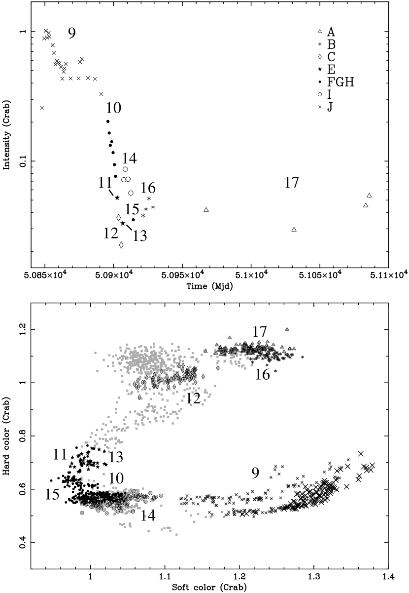
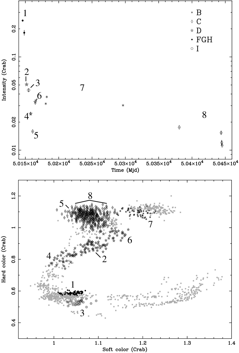
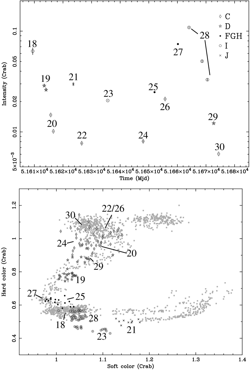


 |
 |
|
 |
 |
 |
 |
|
 |
 |
 |
 |