A New Method for Calculating Arrival Distribution of Ultra-High Energy Cosmic Rays above $10^{19}$ eV with Modifications by the Galactic Magnetic Field

Abstract

We present a new method for calculating arrival distribution of Ultra-High Energy Cosmic Rays (UHECRs) including modifications by the galactic magnetic field. We perform numerical simulations of UHE anti-protons, which are injected isotropically at the earth, in the Galaxy and record the directions of velocities at the earth and outside the Galaxy for all of the trajectories. We then select some of them so that the resultant mapping of the velocity directions outside the Galaxy of the selected trajectories corresponds to a given source location scenario, applying Liouville’s theorem. We also consider energy loss processes of UHE protons in the intergalactic space. Applying this method to our source location scenario which is adopted in our recent study and can explain the AGASA observation above $4\times 10^{19}$ eV, we calculate the arrival distribution of UHECRs including lower energy ($E>10^{19}{\rm eV}$) ones. We find that our source model can reproduce the large-scale isotropy and the small-scale anisotropy on UHECR arrival distribution above $10^{19}$ eV observed by the AGASA. We also demonstrate the UHECR arrival distribution above $10^{19}$ eV with the event number expected by future experiments in the next few years. The interesting feature of the resultant arrival distribution is the arrangement of the clustered events in the order of their energies, reflecting the directions of the galactic magnetic field. This is also pointed out by Alvarez-Muniz, Engel & Stanev (2002). This feature will allow us to obtain some kind of information about the composition of UHECRs and the magnetic field with increasing amount of data.

1 INTRODUCTION

There is no statistically significant large scale anisotropy in the observed arrival distribution of ultra-high energy cosmic rays (UHECRs) above $10^{19}$ eV (Takeda et al., 1999). This may imply an extragalactic origin of cosmic rays above $10^{19}$ eV, combined with the change of spectral slope of the observed energy spectrum at $\sim 10^{19}$ eV (Bird et al., 1994; Yoshida et al., 1995; Takeda et al., 1998). Another important feature of the UHECR arrival distribution is the small scale clusterings of the arrival directions (Takeda et al., 1999, 2001). The current AGASA data set of 57 events above 4 $\times 10^{19}$ eV contains four doublets and one triplet within a separation angle of 2.5^∘. Chance probability to observe such clusters under an isotropic distribution is only about 1 $\%$ (Hayashida et al., 2000; Takeda et al., 2001).

On the other hand, the cosmic-ray energy spectrum does not show the GZK cutoff (Greisen, 1966; Zatsepin & Kuz’min, 1966) because of photopion production with the photons of the cosmic microwave background (CMB) and extends above $10^{20}$ eV (Takeda et al., 1998). The discrepancy between the AGASA and the High Resolution Fly’s Eye (HiRes; Wilkinson et al., 1999), which reports the cosmic ray flux with the GZK cut-off around $10^{20}$ eV (Abu-Zayyad et al., 2002), remains to be one of the major open question in astroparticle physics. This issue is left for future investigation by new large-aperture detectors under development, such as South and North Auger project (Capelle et al., 1998), the EUSO (Benson & Linsley, 1982), and the OWL (Cline & Stecker, 2000) experiments.

In our recent work (Yoshiguchi et al., 2003a, hereafter Paper I), we perform numerical simulations for propagation of UHE protons in intergalactic space, and examine whether the present AGASA observation above $4\times 10^{19}$ eV can be explained by a bottom-up scenario in which the source distribution of UHECRs is proportional to that of galaxies. We use the Optical Redshift Survey (ORS; Santiago et al., 1995) to construct realistic source models of UHECRs.

In Paper I, we calculate both the energy spectrum and arrival directions of UHE protons, and compare the results with the AGASA observation above $4\times 10^{19}$ eV. We find that the large-scale isotropy and the small-scale anisotropy of the UHECR arrival distribution observed by the AGASA can be reproduced when $\sim 1/50$ of the ORS sample more luminous than $-20.5$ mag are selected as UHECR sources, in the case of weak extragalactic magnetic field (EGMF $B\leq 1$ nG). In terms of the source number density, this constraint corresponds to $\sim 10^{-6}$ Mpc^-3.

The small scale anisotropy can not be well reproduced in the case of strong EGMF ($B\geq 10$ nG), because the correlation at small scale between events which originate from a single source is eliminated, or the correlation continues to larger angle scale, due to large deflection when UHECRs propagate in the EGMF from sources to the earth. Although Isola & Sigl (2002) and Sigl, Miniati, & Ensslin (2003) conclude that the expected small-scale anisotropy and large-scale isotropy for local enhancement of UHECR sources in the LSC in the presence of the strong EGMF ($\sim 1\mu$ G) are in marginal agreement with the AGASA, the consistency is somewhat worse than that predicted by our scenario for $B=1$ nG. Of course, we can not draw any firm conclusion about the strength of the EGMF, considering the current limited amount of data. However, we assume extremely weak EGMF throughout the paper.

If local enhancement of UHECR sources in the LSC (Isola & Sigl, 2002; Sigl, Miniati, & Ensslin, 2003) is disfavored from the observations, there is no way that explains the observed extension of the cosmic-ray spectrum beyond the GZK cutoff. Our conclusion in Paper I is that a large fraction of cosmic rays above $10^{20}$ eV observed by the AGASA experiment might originate in the top-down scenarios, or that the energy spectrum measured by the Hires experiment might be better.

As mentioned above, we obtain the constraint on the source number density as $\sim 10^{-6}$ Mpc^-3 by comparing our model prediction with the AGASA data only above $4\times 10^{19}$ eV. It is very important to examine whether our source model can explain the AGASA data including lower energy $(\sim 10^{19}{\rm eV})$ one. On the other hand, the arrival directions of UHECRs above $10^{19}$ eV are modified by the galactic magnetic field (GMF) by a few $-\sim 10$ degrees. In order to accurately calculate the expected UHECR arrival distribution and compare with the observations, the effect of the GMF should be taken into account.

The first step of the studies of UHECR propagation in the GMF is found in Alvarez-Muniz, Engel & Stanev (2002). Alvarez-Muniz, Engel & Stanev (2002) calculate the expected arrival distribution of UHECRs above $10^{19.4}$ eV for several source location scenarios. They perform numerical simulations of UHECR propagation in the Galaxy injected from sources toward the earth. The radius of the earth (detector) must be so small that the unavoidable smearing in arrival angle is kept smaller than the accuracy of arrival direction determination $\sim$ a few degree (Takeda et al., 2001). In this case, the number fraction of injected UHECRs arriving at the earth is very small. This requires a large number of particles to be propagated, which takes enormous CPU time.

In this paper, we present a new method for calculating UHECR arrival distribution which can be applied to several source location scenarios including modifications by the GMF. We numerically calculate the propagation of anti-protons from the earth toward the outside of the Galaxy (in this study, we set a sphere centered around the Galactic center with radius $r_{\rm src}=$40 kpc as the boundary condition), including the effects of Lorentz force due to the GMF. The anti-protons are ejected isotropically from the earth. By this calculation, we can obtain the trajectories and the sky map of position of anti-protons that have reached to the boundary at radius $r_{\rm src}=$ 40 kpc.

Next, we regard the obtained trajectories as the ones of PROTONs from the outside of the galaxy toward the earth. Also, we regard the obtained sky map of position of anti-proton at the boundary as relative probability distribution (per steradian) for PROTONs to be able to reach to the earth for the case in which the flux of the UHE protons from the extra-galactic region is isotropic (in this study, this flux corresponds to the one at the boundary $r_{\rm src}=40$ kpc). This treatment is supported by the Liouville’s theorem. When the flux of the UHE protons at the boundary is anisotropic (e.g., the source distribution is not isotropic), this effect can be included by multiplying this effect (that is, by multiplying the probability density of arrival direction of UHE protons from the extra-galactic region at the boundary) to the obtained relative probability density distribution mentioned above.

By adopting this new method, we can consider only the trajectories of protons which arrive to the earth, which, of course, helps us to save the CPU time efficiently and makes calculation of propagation of CRs even with low energies ($\sim 10^{19}$ eV) possible within a reasonable time. We also consider the energy loss processes of UHE protons in the intergalactic space, which is not taken into account by Alvarez-Muniz, Engel & Stanev (2002).

With this method, we calculate the UHECR arrival distribution above $10^{19}$ eV for our source scenario which can explain the current AGASA observation above $10^{19.6}$ eV. Using the harmonic amplitude and the two point correlation function as statistical quantities, we compare our model prediction with the AGASA observation. We also demonstrate the arrival distribution of UHECRs with the event number expected by future experiments such as South and North Auger project (Capelle et al., 1998), the EUSO (Benson & Linsley, 1982), and the OWL (Cline & Stecker, 2000) experiments.

In section 2, we introduce the GMF model. We explain the method for calculating UHECR arrival distribution in section 3. Results are shown in section 4. In section 5, we summarize the main results.

2 GALACTIC MAGNETIC FIELD

In this study, we adopt the GMF model used by Alvarez-Muniz, Engel & Stanev (2002), which is composed of the spiral and the dipole field. In the following, we briefly introduce this GMF model.

Faraday rotation measurements indicate that the GMF in the disk of the Galaxy has a spiral structure with field reversals at the optical Galactic arms (Beck, 2001). We use a bisymmetric spiral field (BSS) model, which is favored from recent work (Han, Manchester, & Qiao, 1999; Han, 2001). The Solar System is located at a distance $r_{||}=R_{\oplus}=8.5$ kpc from the center of the Galaxy in the Galactic plane. The local regular magnetic field in the vicinity of the Solar System is assumed to be $B_{\rm Solar}\sim 1.5~{}\mu{\rm G}$ in the direction $l=90^{\rm o}+p$ where the pitch angle is $p=-10^{\rm o}$ (Han & Qiao, 1994).

In the polar coordinates $(r_{||},\phi)$, the strength of the spiral field in the Galactic plane is given by

$$B(r_{||},\phi)=B_{0}~{}\left({R_{\oplus}\over r_{||}}\right)~{}\cos\left(\phi-\beta\ln{r_{||}\over r_{0}}\right)$$ (1)

where $B_{0}=4.4~{}\mu$G, $r_{0}=10.55$ kpc and $\beta=1/\tan p=-5.67$. The field decreases with Galactocentric distance as $1/r_{||}$ and it is zero for $r_{||}>20$ kpc. In the region around the Galactic center ($r_{||}<4$ kpc) the field is highly uncertain, and thus assumed to be constant and equal to its value at $r_{||}=4$ kpc.

The spiral field strengths above and below the Galactic plane are taken to decrease exponentially with two scale heights (Stanev, 1996)

$$|B(r_{||},\phi,z)|=|B(r_{||},\phi)|\left\{\begin{array}[]{lcl}\exp(-z):&|z|\leq 0.5~{}{\rm kpc}\\ \exp(\frac{-3}{8})~{}\exp(\frac{-z}{4}):&|z|>0.5~{}{\rm kpc}\end{array}\right.$$ (2)

where the factor $\exp(-3/8)$ makes the field continuous in $z$. The BSS spiral field we use is of even parity, that is, the field direction is preserved at disk crossing.

Observations show that the field in the Galactic halo is much weaker than that in the disk. In this work we assume that the regular field corresponds to a A0 dipole field as suggested in (Han, 2002). In spherical coordinates $(r,\theta,\varphi)$ the $(x,y,z)$ components of the halo field are given by:

$$B_{x}=-3~{}\mu_{\rm G}~{}{\sin\theta\cos\theta\cos\varphi}/r^{3}$$

$$B_{y}=-3~{}\mu_{\rm G}~{}{\sin\theta\cos\theta\sin\varphi}/r^{3}$$ (3)

$$B_{z}=\mu_{\rm G}~{}{(1-3\cos^{2}\theta)}/r^{3}~{}~{}~{}~{}~{}~{}~{}$$

where $\mu_{\rm G}\sim 184.2~{}{\rm\mu G~{}kpc^{3}}$ is the magnetic moment of the Galactic dipole. The dipole field is very strong in the central region of the Galaxy, but is only 0.3 $\mu$G in the vicinity of the Solar system, directed toward the North Galactic Pole.

There is a significant turbulent component, $B_{\rm ran}$, of the Galactic magnetic field. Its field strength is difficult to measure and results found in literature are in the range of $B_{\rm ran}=0.5\dots 2B_{\rm reg}$ (Beck, 2001). However, we neglect the random field throughout the paper, in order to make easy to see the effects of the regular field, such as the arrangement of the clustered event in the order of their energies (section 4.3). Possible dependence of the results on the random field is discussed in the section 4.2.

3 NUMERICAL METHOD

3.1 Propagation of UHECRs in the Intergalactic Space

The energy spectrum of UHECRs injected at extragalactic sources is modified by the energy loss processes when they propagate in the intergalactic space. This subsection provides the method of Monte Carlo simulations for propagation of UHE protons in intergalactic space.

We assume that UHECRs are protons injected with a power law spectrum within the range of ($10^{19}$ - $10^{22}$)eV. 10000 protons are injected in each of 31 energy bins, that is, 10 bins per decade of energy. Then, UHE protons are propagated including the energy loss processes (explained below) over $3$ Gpc for $15$ Gyr. We take a power law index as 2.6 in order to fit the calculated energy spectrum to the one observed by the AGASA (Marco, Blasi, & Olinto, 2003).

UHE protons below $\sim 8\times 10^{19}$ eV lose their energies mainly by pair creations and adiabatic energy losses, and above it by photopion production (Berezinsky & Grigorieva, 1988; Yoshida & Teshima, 1993) in collisions with photons of the CMB. We treat the adiabatic loss as a continuous loss process. We calculate the redshift $z$ of source at a given distance using the cosmological parameters $H_{0}=71$ km s^-1 Mpc^-1, $\Omega_{m}=0.27$, and $\Omega_{\Lambda}=0.73$. Similarly, the pair production can be treated as a continuous loss process considering its small inelasticity ($\sim 10^{-3}$). We adopt the analytical fit functions given by Chodorowski, Zdziarske, & Sikora (1992) to calculate the energy loss rate for the pair production on isotropic photons. The same approach has been adopted in our previous studies (Paper I, Ide et al., 2001; Yoshiguchi, Nagataki, & Sato, 2003c).

On the other hand, protons lose a large fraction of their energy in the photopion production. For this reason, its treatment is very important. We use the interaction length and the energy distribution of final protons as a function of initial proton energy which is calculated by simulating the photopion production with the event generator SOPHIA (Mucke et al., 2000).

In this study, we neglect the effect of the EGMF because of the following two reasons. First, numerical simulations of UHECR propagation in the EGMF including lower energy ($\sim 10^{19}$ eV) ones take a long CPU time. Second, we show in our previous study that small scale clustering can be well reproduced in the case of weak EGMF $(B<1{\rm nG})$ (Paper I). Isola & Sigl (2002) and Sigl, Miniati, & Ensslin (2003) show that the expected small scale anisotropy for local enhancement scenario of UHECR sources in the presence of strong EGMF ($\sim 1\mu$ G) in the Local Super Cluster is marginally consistent with the AGASA observation. However, the consistency of small-scale anisotropy is somewhat worse than that predicted by our scenario in the case of weak EGMF (Paper I). Although we can not draw any firm conclusion because of the limited amount of data, we assume extremely weak EGMF throughout the paper.

3.2 Source Distribution

In this study, we apply the method for calculating the UHECR arrival distribution with modifications by the GMF (section 3.3) to our source location scenario, which is constructed by using the ORS (Santiago et al., 1995) galaxy catalog. As mentioned in section 1, we show in Paper I that the arrival distribution of UHECRs observed by the AGASA can be reproduced when $\sim 1/50$ of the ORS galaxies more luminous than $M_{\rm lim}=-20.5$ is selected as UHECR sources. We consider only this source model throughout the paper. It is unknown how much an ultimate UHECR source contribute to the observed cosmic ray flux. In paper I, we thus consider the two cases in which (1) all galaxies inject the same amount of cosmic rays, or (2) they inject cosmic rays proportionally to their absolute luminosity. However, we find that the results in the two cases do not differ from each other, as far as we focus on the luminous galaxies as UHECR sources. Accordingly, we restrict ourselves to the case that all galaxies inject the same amount of cosmic rays.

In order to calculate the energy spectrum and the distribution of arrival directions of UHECRs realistically, there are two key elements of the galaxy sample to be corrected. First, galaxies in a given magnitude-limited sample are biased tracers of matter distribution because of the flux limit (Yoshiguchi et al., 2003b). Although the sample of galaxies more luminous than $-20.5$ mag is complete within 80 $h^{-1}$ Mpc (where $h$ is the Hubble constant divided by 100 km s^-1 and we use $h=0.71$), it does not contain galaxies outside it for the reason of the selection effect. We distribute sources of UHECRs outside 80 $h^{-1}$ Mpc homogeneously. Their number density is set to be equal to that inside 80 $h^{-1}$ Mpc. We do not take into account luminosity evolution for simplicity.

Second, our ORS sample does not include galaxies in the zone of avoidance ($|b|<20^{\circ}$). In the same way, we distribute UHECR sources in this region homogeneously, and calculate its number density from the number of galaxies in the observed region.

3.3 Calculation of the UHECR Arrival Distribution with modifications by the GMF

In this subsection, we present the method of calculation of UHECR arrival distribution with modifications by the GMF. We start by injecting anti-protons from the earth isotropically, and follow each trajectory until

1. anti-proton reaches a sphere of radius $40$ kpc centered at the galactic center, or

2. the total path length traveled by anti-proton is larger than $200$ kpc,

by integrating the equations of motion in the magnetic field. It is noted that we regard these anti-protons as PROTONs injected from the outside of the Galaxy toward the earth. The number of propagated anti-proton is 2,000,000. We have checked that the number of trajectories which are stopped by the limit (2) is smaller than $0.1$% of the total number. The energy loss of protons can be neglected for these distances. Accordingly, we inject anti-protons with injection spectrum similar to the observed one $\sim E^{-2.7}$. (Note that this is not the energy spectrum injected at extragalactic sources.)

The result of the velocity directions of anti-protons at the sphere of radius $40$ kpc is shown in the right panel of figure 1 in the galactic coordinate. From Liouville’s theorem, if the cosmic-ray flux outside the Galaxy is isotropic, one expects an isotropic flux at the earth even in the presence of the GMF. This theorem is confirmed by numerical calculations shown in figure 6 of Alvarez-Muniz, Engel & Stanev (2002), which is the same figure as our figure 1 except for threshold energy. Thus, the mapping of the velocity directions in the right panel of figure 1 corresponds to the sources which actually give rise to the flux at the earth in the case that the sources (including ones which do not actually give rise to the flux at the earth) are distributed uniformly.

Figure 1: Arrival directions of anti-protons with $E>10^{19.0}$ eV at the sphere of Galactocentric radius of $40$ kpc (right panel) in the galactic coordinate. The anti-protons are injected at the earth isotropically (as shown in the left panel) with an injection spectrum $E^{-2.7}$.

We calculate the UHECR arrival distribution for our source scenario using the numerical data of the propagation of UHE anti-protons in the Galaxy. Detailed method is as follows. At first, we divide the sky into a number of bins with the same solid angle. The number of bins is taken to be $360(l)\times 200(b)$. We then distribute all the trajectories into each bin according to their directions of velocities (source directions) at the sphere of radius $40$ kpc. Finally, we randomly select trajectories from each bin with probability $P_{\rm selec}(j,k,E)$ defined as

$$P_{\rm selec}(j,k,E)\propto\sum_{i}\frac{1}{d_{i}^{2}}\,\frac{dN/dE(d_{i},E)}{E^{-2.7}}.$$ (4)

Here subscripts j and k distinguish each cell of the sky, $d_{i}$ is distance of each galaxy within the cell of (j,k), and the summation runs over all of the galaxies within it. $E$ is the energy of proton, and $dN/dE(d_{i},E)$ is the energy spectrum of protons at our galaxy injected at a source of distance $d_{i}$.

The normalization of $P_{\rm selec}(j,k,E)$ is determined so as to set the total number of events equal to a given number, for example, the event number of the current AGASA data. When $P_{\rm selec}>1$, we newly generate events with number of $(P_{\rm selec}-1)\times N(j,k)$, where $N(j,k)$ is the number of trajectories within the sky cell of $(j,k)$. The arrival angle of newly generated proton (equivalently, injection angle of anti-proton) at the earth is calculated by adding a normally distributed deviate with zero mean and variance equal to the experimental resolution $2.8^{\circ}$ $(1.8^{\circ})$ for $E>10^{19}$ eV $(4\times 10^{19}{\rm eV})$ to the original arrival angle. We perform this event generation 20 times in order to calculate the averages and variances, due to the finite number of the simulated events, of the statistical quantities (section 3.4).

3.4 Statistical Methods

In this subsection, we explain the two statistical quantities, the harmonics analysis for large scale anisotropy (Hayashida et al., 1999), the two point correlation function for small scale anisotropy.

The harmonic analysis to the right ascension distribution of events is the conventional method to search for global anisotropy of cosmic ray arrival distribution. For a ground-based detector like the AGASA, the almost uniform observation in right ascension is expected. The $m$-th harmonic amplitude $r$ is determined by fitting the distribution to a sine wave with period $2\pi/m$. For a sample of $n$ measurements of phase, $\phi_{1}$, $\phi_{2}$, $\cdot\cdot\cdot$, $\phi_{n}$ (0 $\leq\phi_{i}\leq 2\pi$), it is expressed as

$$r=(a^{2}+b^{2})^{1/2}$$ (5)

where, $a=\frac{2}{n}\Sigma_{i=1}^{n}\cos m\phi_{i}$, $b=\frac{2}{n}\Sigma_{i=1}^{n}\sin m\phi_{i}$. We calculate the harmonic amplitude for $m=1,2$ from a set of events generated by the method explained in the section 3.3.

If events with total number $n$ are uniformly distributed in right ascension, the chance probability of observing the amplitude $\geq r$ is given by,

$$P=\exp(-k),$$ (6)

where

$$k=nr^{2}/4.$$ (7)

The current AGASA 775 events above $10^{19}$ eV is consistent with isotropic source distribution within 90 $\%$ confidence level (Takeda et al., 2001). We therefore compare the harmonic amplitude for $P=0.1$ with the model prediction.

The two point correlation function $N(\theta)$ contains information on the small scale anisotropy. We start from a set of generated events. For each event, we divide the sphere into concentric bins of angular size $\Delta\theta$, and count the number of events falling into each bin. We then divide it by the solid angle of the corresponding bin, that is,

$$N(\theta)=\frac{1}{2\pi|\cos\theta-\cos(\theta+\Delta\theta)|}\sum_{\theta\leq\phi\leq\theta+\Delta\theta}1\;\;\;[\rm sr^{-1}],$$ (8)

where $\phi$ denotes the separation angle of the two events. $\Delta\theta$ is taken to be $1^{\circ}$ in this analysis. The AGASA data shows correlation at small angle $(\sim 3^{\circ})$ with 2.3 (4.6) $\sigma$ significance of deviation from an isotropic distribution for $E>10^{19}$ eV $(E>4\times 10^{19}{\rm eV})$ (Takeda et al., 2001).

4 RESULTS

4.1 Arrival Distribution of UHECRs above $10^{19}$ eV

In this subsection, we present the results of the arrival distribution of UHECRs above $10^{19}$ eV, using the method explained in the section 3.3. At first, figure 2 shows the distribution of the sources for a specific source selection when $\sim 1/50$ of the ORS galaxies more luminous than $M_{\rm{lim}}=-20.5$ is randomly selected as UHECR sources in the galactic coordinate. We show only the sources within $300$ Mpc from us for clarity, as circles of radius inversely proportional to their distances. It is noted that the sources outside 113$(=80h^{-1})$ Mpc are randomly distributed because the ORS sample does not contain any galaxy outside it.

Figure 2: Distribution of the sources in our model in the galactic coordinate. We show only the sources within $300$ Mpc from us as circles of radius inversely proportional to their distances. It is noted that the sources outside 113$(=80h^{-1})$ Mpc are randomly distributed because the ORS sample does not contain any galaxy outside it.

Energy spectrum with injection spectrum $E^{-2.6}$, predicted by the source model of figure 2. The contributions from sources at different distances are also shown. We also show the observed cosmic-ray spectrum by the AGASA experiments (Hayashida et al., 2000).

We show in figure 4.1 the expected energy spectrum for the source model of figure 2. The injection spectrum is set to be $E^{-2.6}$. The contributions from sources at different distances are also shown. We also show the observed cosmic-ray spectrum by the AGASA experiments (Hayashida et al., 2000). The resultant spectrum is in good agreement with the one observed by the AGASA, except for $E>10^{20}$ eV. As mentioned above, we conclude in Paper I that a large fraction of cosmic rays above $10^{20}$ eV observed by the AGASA experiment might originate in the top-down scenarios. Accordingly, we consider only cosmic rays with $E<10^{20}$ eV throughout the paper.

As mentioned above, Alvarez-Muniz, Engel & Stanev (2002) does not take the energy loss processes in the intergalactic space into account. Thus, they can not include the effects of difference between resultant energy spectra injected at different distances into numerical calculations. In our calculations, however, sources at larger distance mainly contribute to the cosmic ray flux at lower energies as is evident from figure 4.1. This enables us to calculate the arrival distribution of UHECRs under more realistic situations.

Given the source distribution and the resultant energy spectrum as a function of the source distance, we can calculate the right hand side of Eq. 4. Then we perform the selection of trajectories according to the probability $P_{\rm selec}$, as explained in the section 3.3.

One realization of the event generations is shown in figure 3. The events are shown by color according to their energies. This figure corresponds to figure 1. That is, the injection directions of anti-protons at the earth (figure 1, left) corresponds to the arrival directions of protons (figure 3, left). Similarly, the arrival directions of anti-protons at the sphere of Galactocentric radius of $40$ kpc (figure 1, right) does to the directions of the sources which actually give rise to the cosmic-ray flux (figure 3, right).

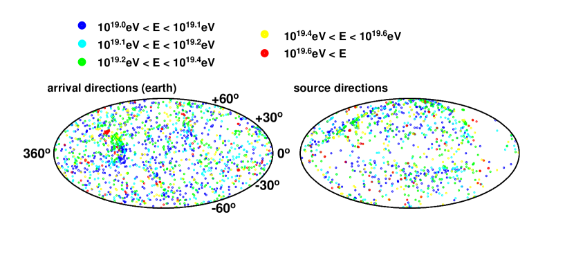
Figure 3: Arrival directions of protons with $E>10^{19.0}$ eV at the earth (left panel) expected for the source model of figure 2 in the galactic coordinate. The events are shown by color according to their energies. The event number within $-10^{\circ}\leq\delta\leq 80^{\circ}$ is set to be equal to the one observed by the AGASA (Takeda et al., 2001, 775) (The total number of events is $\sim 1500$). The right panel is the mapping of the sources which actually give rise to events shown in the left panel. Note that this mapping differ from the distribution of the sources shown in figure 2.

For the source model of figure 2, the nearest source is located at $(b,l)=(31^{\circ},284^{\circ})$ and 64 Mpc from us. A number of the simulated events are clustered at this direction as seen in figure 3. Furthermore, these events are aligned in the sky according to the order of their energies, reflecting the direction of the GMF at this direction. As we will show in the section 4.3, this interesting feature of the UHECR arrival distribution becomes evident with increasing amount of the event number.

4.2 Statistics on the UHECR Arrival Distribution

In this subsection, we show the results of the statistical quantities on the UHECR arrival distribution above $10^{19}$ eV. In the last section, we showed the results for a specific source scenario when $\sim 1/50$ of the ORS galaxies more luminous than $M_{\rm{lim}}=-20.5$ is randomly selected as UHECR sources. However, the statistical quantities presented in this section are calculated with not only the statistical error but also the variation between different selections of source from our ORS sample.

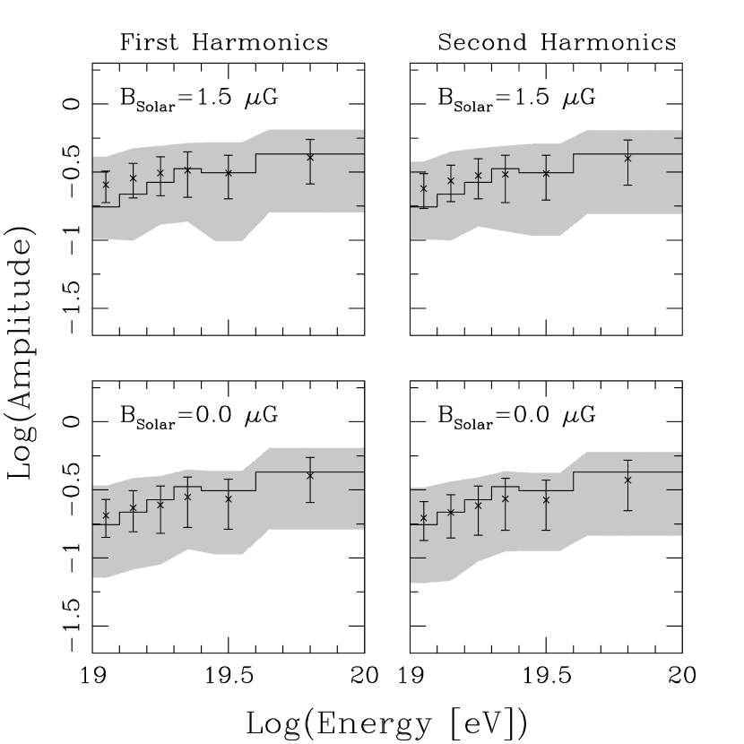
Figure 4: Harmonic amplitude predicted by our source model as a function of the cosmic-ray energies. The errorbars represent the statistical fluctuations due to the finite number of the simulated events, which is set to be equal to that observed by the AGASA within $-10^{\circ}\leq\delta\leq 80^{\circ}$. The shaded regions represent 1 $\sigma$ total error due to not only the statistical error but also the source selections from our ORS sample. The region below the solid line is expected values due to the statistical fluctuation of isotropic source distribution with the chance probability larger than 10$\%$.

The upper panels of figure 4 shows the first and the second harmonics predicted by our source model as a function of the cosmic-ray energies for $B_{\rm Solar}=1.5\mu$ G, where $B_{\rm Solar}$ is the strength of the GMF in the vicinity of the Solar system. It is noted that we calculate the harmonic amplitudes for the simulated events within only $-10^{\circ}\leq\delta\leq 80^{\circ}$ in order to compare with AGASA data. The errorbars represent the statistical fluctuations due to the finite number of the simulated events, which is set to be equal to that observed by the AGASA (775 events for $E>10^{19}$ eV). The event selections are performed $20$ times. The shaded regions represent 1 $\sigma$ total error due to not only the statistical error but also the source selections from our ORS sample. The random source selections are performed $100$ times. The region below the histogram is expected values for the statistical fluctuation of isotropic source distribution with the chance probability larger than 10$\%$.

It is clear that our source model predicts the large-scale isotropy fully consistent with that expected by uniform source distribution within 1 $\sigma$ total error (statistical one plus source selection). We have checked that 27 source distributions out of 100 predict the sufficient large-scale isotropy within 1 $\sigma$ statistical error. In order to investigate the effects of the GMF on the large-scale anisotropy, we also calculate the harmonic amplitude for the case of $B_{\rm Solar}=0.0\mu$ G. For $B_{\rm Solar}=0.0\mu$ G, the predicted arrival distribution is relatively more isotropic than that for $B_{\rm Solar}=1.5\mu$ G. We also note that this tendency can be seen at lower energies ($\sim 10^{19}$ eV). Because the deflection angle of cosmic rays with such energies by the GMF is about $\sim{\rm afew}\times 10^{\circ}$, the harmonic amplitude of arrival distribution of UHECRs can be affected by anisotropy of the event distributions which is caused by the events aligned according to the order of their energies, reflecting the direction of the GMF.

Two point correlation function expected for our source model for $E>4\times 10^{19}$ (left) and $E>10^{19}$ eV (right). The errorbars represent the statistical fluctuations due to the finite number of the simulated events, which is set to be equal to that observed by the AGASA within $-10^{\circ}\leq\delta\leq 80^{\circ}$. The shaded regions represent 1 $\sigma$ total error due to not only the statistical error but also the source selections from our ORS sample. The histograms represent the AGASA data. However, the AGASA data for $E>10^{19}$ eV are fitted to the result of our calculation at larger angle ($30^{\circ}$), since we can not know the normalization of the AGASA data with this energy.

In figure 4.2, we show two point correlation function predicted by our source model for $E>4\times 10^{19}$ (left) and $E>10^{19}$ eV (right). It is noted that we calculate two point correlation function for the simulated events within only $-10^{\circ}\leq\delta\leq 80^{\circ}$ in order to compare with AGASA data. The errorbars represent the statistical fluctuations due to the finite number of the simulated events, which is set to be equal to that observed by the AGASA (775 events for $E>10^{19}$ eV). The shaded regions represent 1 $\sigma$ total error due to not only the statistical error but also the source selections from our ORS sample. The event selections and the random source selections are performed $20$ times and $100$ times, respectively. The event numbers shown in this figures are averaged over all trials of the event selections and the source selections. The histograms represent the AGASA data. However, the AGASA data for $E>10^{19}$ eV are fitted to the result of our calculation at larger angle ($30^{\circ}$), since we can not know the normalization of the AGASA data with this energy.

Clearly visible is that large peak at small angle scale is too strong compared with the AGASA observation (Takeda et al., 2001). We have checked that when extremely nearby sources are selected by accident, predicted small-scale anisotropy becomes to be very strong. This is the reason for too large peak at small angle scale in figure 4.2, where the averages and the variances are calculated including such source distributions.

Provided that extremely nearby sources are selected by accident, not only the small-scale anisotropy but also the large-scale isotropy is inconsistent with the AGASA observation. Accordingly, we calculate two point correlation function only for the source distributions which predict the large-scale isotropy consistent with uniform source distribution within 1 $\sigma$ statistical error. The number of such source distributions is 27 out of all the 100 source selections. The result is shown in figure 4.2.

Two point correlation function in figure 4.2 exhibits a structure that is similar to that seen in the AGASA data, that is, large peak at small angle scale followed by a tail at large angles. For $E>10^{19}$ eV, a peak at small angles is somewhat weaker than that for $E>4\times 10^{19}$ eV because of the large deflection by the GMF. This feature is also seen in AGASA data (Takeda et al., 2001). From this result, it can be understood that the source distributions which predict sufficient large-scale isotropy also predict the small-scale anisotropy that is similar to that seen in the AGASA data.

Same as figure 4.2. But, this is the result only for source distributions which predict the large-scale anisotropy consistent with uniform source distribution within 1 $\sigma$ statistical error.

However, we should note that the peak at small angle scale is still relatively strong compared with the AGASA. There may be two possible explanations for this fact. First, we neglect the effects of the extragalactic magnetic field in this study, in order to save the CPU time. If we can include this effect by future studies, strong correlation at small scale will be reduced because of the deflection of UHECRs in the intergalactic space. Second, we also neglect the random component of the GMF in order to make easy to see the effect of the regular field. This may also relax the large peak at small angle scale, provided that there is the random component with same level of strength with the regular component. These issues are left for future investigations.

4.3 Future Prospects of UHECR arrival distribution

In this subsection, we demonstrate the results of the UHECR arrival distribution above $E>10^{19}$ eV with the event number expected by future experiments, such as Auger, EUSO and OWL. The results for the source model of figure 2 are shown in figure 5. The events are shown by color according to their energies. It is noted that the expected event rate by the Auger experiment is $\sim 3000$ per year above $10^{19}$ eV. These results are extended versions of our previous study (Yoshiguchi, Nagataki, & Sato, 2003c), where we predict the UHECR arrival distribution above $4\times 10^{19}$ eV without modifications by the GMF.

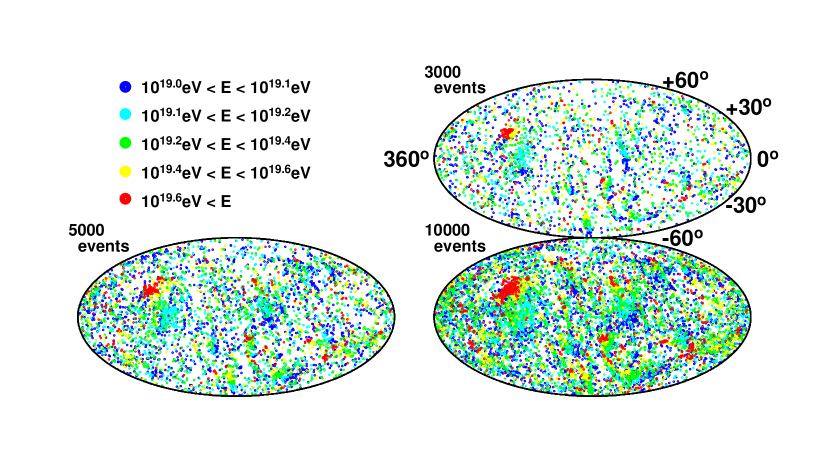
Figure 5: Arrival directions of protons with $E>10^{19.0}$ eV at the earth expected for the source model of figure 2 in the galactic coordinate. The events are shown by color according to their energies. It is noted that the expected event rate by the Auger experiment is $\sim 3000$ per year above $10^{19}$ eV.

Remarkable feature is the arrangement of clustered events at the directions of nearby sources (see figure 2). The events are aligned according to the order of their energies reflecting the direction of the GMF. We will be able to obtain some kind of information about the GMF and the chemical composition of UHECRs. In forthcoming work, we plan studies about new statistical quantities which allow us to obtain such invaluable information.

5 SUMMARY AND DISCUSSION

In this paper, we presented a new method for calculating the arrival distribution of UHECRs, which can be applied to several source location scenarios, including modifications by the GMF. We performed numerical simulations of UHE anti-protons, which are injected isotropically at the earth, in the Galaxy and recorded the directions of velocities at the earth and outside the Galaxy for all of the trajectories. It is noted that we regard these anti-protons as PROTONs injected from the outside of the Galaxy toward the earth. We then selected some trajectories so that the resultant mapping of the velocity directions outside the Galaxy of the selected trajectories corresponds to our source location scenario, applying Liouville’s theorem.

There are two points of our improvement over the work of Alvarez-Muniz, Engel & Stanev (2002). First, we calculated only the trajectories actually reaching the detectors by propagating anti-protons backwards from Earth, instead of propagating protons from the source and selecting those reaching the Earth. This helps us to save the CPU time efficiently and makes calculations of propagation of cosmic rays even with lower energies ($\sim 10^{19}$ eV) possible within a reasonable time. Second, we considered energy loss processes of UHE protons in the intergalactic space, which is not taken into account in Alvarez-Muniz, Engel & Stanev (2002). This enables us to include the effects of difference between resultant energy spectra injected at different distances into numerical calculations. We can calculate the arrival distribution of UHECRs under more realistic situation.

As an application of this method, we calculate the UHECR arrival distribution above $10^{19}$ eV for the source model which is adopted in our recent study (Paper I) and can explain the current AGASA observation above $4\times 10^{19}$ eV. We found that the predicted large-scale anisotropy is fully consistent with uniform source distribution, in the same manner as the current AGASA data. In order to investigate the effects of the GMF on the large-scale anisotropy, we calculated the harmonic amplitude for the case of $B_{\rm Solar}=0.0\mu$ G. For $B_{\rm Solar}=0.0\mu$ G, the predicted arrival distribution is relatively more isotropic than that for $B_{\rm Solar}=1.5\mu$ G. This would be due to anisotropy of the event distributions which is caused by the events aligned according to the order of their energies, reflecting the direction of the GMF.

It is also found that the calculated two point correlation function is similar to that of AGASA data, when we restrict our attention to the source distributions which predict sufficient isotropic arrival distribution of UHECRs. There may be effects of the extragalactic magnetic field and the random component of the GMF on the large peak of two point correlation function. These issues are left for future studies.

Finally, we demonstrated the UHECR arrival distribution above $10^{19}$ eV with the event number expected by future experiments in the next few years. The interesting feature of the resultant arrival distribution is the events aligned according to the order of their energies, reflecting the directions of the galactic magnetic field. This is also pointed out by Alvarez-Muniz, Engel & Stanev (2002). This feature will become clear with increasing amount of data, and allow us to obtain some kind of information about the composition of UHECRs and the GMF. In forthcoming work, we plan studies about new statistical quantities which allow us to obtain such invaluable information.

In the present work, we calculate the arrival distribution of UHECRs for our source location scenario which is adopted in our previous study (Paper I). However, it should be mentioned that the same results would be obtained if the sources were truly drawn at random, as far as the source number density is $\sim 10^{-6}$ Mpc^-3. The results such as the events aligned according to the order of their energies are independent on our assumption about the source distribution.

In this study, we calculate the harmonic amplitude and two point correlation function, which are only published quantities on UHECRs observed by the AGASA including lower energy ones ($\sim 10^{19}$ eV). In particular, the AGASA observation has published neither existence nor non-existence of the events aligned according to the order of their energies. If more detailed event data with $E<4\times 10^{19}$ eV are published, we may obtain more strong constraint on our source model, other than the source number density, using another statistical quantities. This is also one of future study plans.

References

- Abu-Zayyad et al. (2002) Abu-Zayyad T. et al. (The HiRes Collaboration) 2002, astro-ph/0208243
- Alvarez-Muniz, Engel & Stanev (2002) Alvarez-Muniz J., Engel R., & Stanev T. 2002, ApJ, 572, 185
- Beck (2001) Beck R. 2001, Space. Sci. Rev. 99, 243
- Benson & Linsley (1982) Benson R., & Linsley J. 1982, A&A, 7, 161
- Berezinsky & Grigorieva (1988) Berezinsky V., & Grigorieva S.I. 1988, A&A, 199, 1
- Bird et al. (1994) Bird D.J., et al. 1994, ApJ, 424, 491
- Capelle et al. (1998) Capelle K.S., Cronin J.W., & Parente G., Zas E. 1998, APh, 8, 321
- Chodorowski, Zdziarske, & Sikora (1992) Chodorowski M.J., Zdziarske A.A., & Sikora M. 1992, ApJ, 400, 181
- Cline & Stecker (2000) Cline D.B., & Stecker F.W. OWL/AirWatch science white paper, astro-ph/0003459
- Greisen (1966) Greisen K. 1966, Phys. Rev. Lett., 16, 748
- Han & Qiao (1994) Han J.L., & Qiao G.J. 1994, A&A, 288, 759
- Han, Manchester, & Qiao (1999) Han J.L., Manchester R.N., & Qiao G.J. 1999, MNRAS, 306, 371
- Han (2001) Han J.L., 2001, Ap&SS, 278, 181
- Han (2002) Han J.L., 2002, astro-ph/0110319.
- Hayashida et al. (1999) Hayashida N., et al. 1999 APh, 10, 303
- Hayashida et al. (2000) Hayashida N., et al. 2000, astro-ph/0008102
- Ide et al. (2001) Ide Y., Nagataki S., Tsubaki S., Yoshiguchi H., & Sato K. 2001, PASJ, 53, 1153
- Isola & Sigl (2002) Isola C., & Sigl G. 2002, astro-ph/0203273
- Marco, Blasi, & Olinto (2003) Marco D.D., Blasi P., & Olinto A.V. 2003, astro-ph/0301497
- Mucke et al. (2000) Mucke A., Engel R., Rachen J.P., Protheroe R.J., & Stanev T. 2000, Comput. Phys. Commun. 124, 290
- Santiago et al. (1995) Santiago B.X., Strauss M.A., Lahav O., Davis M., Dressler A., & Huchra J.P. 1995, ApJ, 446, 457
- Sigl, Miniati, & Ensslin (2003) Sigl G., Miniati F., & Ensslin T.A. 2003, astro-ph/0302388
- Stanev (1996) Stanev T. 1996, ApJ, 479, 290
- Takeda et al. (1998) Takeda M., et al. 1998, Phys. Rev. Lett., 81, 1163
- Takeda et al. (1999) Takeda M., et al. 1999, ApJ, 522, 225
- Takeda et al. (2001) Takeda M., et al. 2001, Proceeding of ICRC 2001, 341
- Wilkinson et al. (1999) Wilkinson C.R., et al. 1999, APh, 12, 121
- Yoshida & Teshima (1993) Yoshida S., & Teshima M. 1993, Prog. Theor. Phys. 89, 833
- Yoshida et al. (1995) Yoshida S., et al. 1995 Astropart. Phys., 3, 105
- Yoshiguchi et al. (2003a) Yoshiguchi H., Nagataki S., Tsubaki S., & Sato K. 2003a, ApJ, 586, 1231 (Paper I, astro-ph/0210132)
- Yoshiguchi et al. (2003b) Yoshiguchi H., Nagataki S., Sato K., Ohama N., & Okamura S. 2003b, PASJ, 55, 121 (astro-ph/0212061)
- Yoshiguchi, Nagataki, & Sato (2003c) Yoshiguchi H., Nagataki S., Sato K. 2003c, ApJ, in press (astro-ph/0302508)
- Zatsepin & Kuz’min (1966) Zatsepin G.T., & Kuz’min V.A. 1966, JETP Lett., 4, 78