Abstract

The nature of the fuel that drives today’s cosmic acceleration is an open and tantalizing mystery. We entertain the suggestion that the acceleration is not the manifestation of yet another new ingredient in the cosmic gas tank, but rather a signal of our first real lack of understanding of gravitational physics. By requiring that the underlying gravity theory respects Birkhoff’s law, we derive the modified gravitational force-law necessary to generate any given cosmology, without reference to the fundamental theory, revealing modifications of gravity at scales typically much smaller than today’s horizon. We discuss how through these modifications, the growth of density perturbations, the late-time integrated Sachs–Wolfe effect, and even solar-system measurements may be sensitive to whether today’s cosmic acceleration is generated by dark energy or modified gravitational dynamics, and are subject to imminent observational discrimination. We argue how these conclusions can be more generic, and probably not dependent on the validity of Birkhoff’s law.

I Introduction

The discovery of a contemporary cosmic acceleration [1, 2] is one of the most profound scientific observations of the latter part of the last century. What drives that acceleration remains an open and tantalizing question. A “conventional” explanation exists for the cause of that acceleration: vacuum energy provides the necessary repulsive gravity in general relativity to drive an accelerated expansion of the universe. Variations on this vacuum-energy theme, e.g. quintessence, promote the energy density to the potential energy density of a dynamical field. Such additions to the roster of cosmic sources of energy-momentum are collectively referred to as dark energy. Accounted for as such, dark energy would constitute the majority of the energy density of the universe today.

However, what if one were to view the current cosmic expansion not as yet another ingredient in our already complex cosmic soup, but rather as a signal of our first real lack of understanding of gravitational physics? (Although others have argued that dark matter was that first signal of post-Einsteinian gravity [3, 4], we will not address ourselves here to that possibility.) An instructive example along that direction is the braneworld theory [5] of Dvali, Gabadadze, and Porrati (DGP). In this theory, gravity appears four-dimensional at short distances but is altered at large distances through the slow evaporation of the graviton off our four-dimensional braneworld universe into an unseen, yet large, fifth dimension [5, 6, 7]. DGP gravity provides an alternative explanation for today’s cosmic acceleration [8, 9]: just as gravity is conventional four-dimensional gravity at short scales and appears five-dimensional at large distance scales, so too the Hubble scale, $H(t)$, evolves by the conventional Friedmann equation at high Hubble scales but saturates at a fixed value as $H(t)$ approaches a value equivalent to the inverse of the crossover distance between four and five-dimensional behavior, $r_{c}^{-1}$. Thus, if one were to set that crossover distance scale to be on the order of $H_{0}^{-1}$, where $H_{0}$ is today’s Hubble scale, DGP could account for today’s cosmic acceleration in terms of the existence of extra dimensions and a modifications of the laws of gravity.

We would naively expect not to be able to probe this extra dimension at distances much smaller than the crossover scale $r_{c}=H_{0}^{-1}$. However, in DGP, although gravity is four-dimensional at distances shorter than $r_{c}$, it is not four-dimensional Einstein gravity – it is augmented by the presence of an ultra-light gravitational scalar. One only recovers Einstein gravity in a subtle fashion [10, 11, 12, 13], and a marked departure from Einstein gravity persists down to distances much shorter than $r_{c}$. For example, for $r_{c}=H_{0}^{-1}$ and a central mass source of Schwarzschild radius $r_{g}$, significant and cosmologically-sensitive deviations from Einstein gravity occur at distances greater than [12, 13, 14, 15]

$$r_{*}=\left(r_{g}r_{c}^{2}\right)^{1/3}=\left({r_{g}\over H_{0}^{2}}\right)^{1/3}\ .$$ (1)

Thus a marked departure from conventional physics persists down to scales much smaller than the distance at which the extra dimension is naively hidden, or for our discussion here, the distance at which the Friedmann equation was modified to account for accelerated cosmic expansion. (Other theories have since shown how alternative modifications of gravity at large distances can lead to late-time acceleration without dark energy [16, 17].)

Recently, appeals have been made to a direct empirical modification of the Friedmann equation in order to explain cosmic acceleration without dark energy [18, 19, 20], broadening the theme explicitly and completely realized by DGP braneworlds. Unfortunately, fully self-consistent models implementing these ideas have yet to be found that can reproduce the desired general modifications to the Friedmann equation, making it difficult to establish the full consequence of the proposed new physics. An important question to be asked is whether gravity theories that produce such modified Friedmann equations can be devoid of observable consequences other than late-time acceleration? There may be something to be learned from the example of DGP gravity. Will these new theories generically lead to similar deviations from Einstein gravity at scales much smaller than today’s Hubble radius?

Pursuing this line of thought without an underlying model is difficult, but not altogether impossible. In this paper, we allow ourselves an assumption about the structure of a possible modified theory of gravity, taking the constraint of Birkhoff’s law as the example, and show how with that assumption alone, one may kinematically ascertain gravitational force interactions, avoiding reference to fundamental dynamics. We then describe how modification of cosmology at today’s Hubble scale can naturally affect gravitational physics at much smaller (e.g. astrophysical, and even under certain circumstances solar system) distance scales. It is worth noting that DGP gravity does not respect Birkhoff’s law, and we conclude with a discussion on how short-distance modifications of gravitational interactions may be a general consequence of gravity modified at cosmological scales.

II The Friedmann Equation and the Force Law

The premise of our approach is that the static, Schwarzschild-like metric, or more specifically its geodesics, may completely determine cosmological evolution, i.e., that the cosmological evolution is driven not by some dark energy background, but by the matter content itself. This should be a familiar premise – it underlies the usual undergraduate-level derivation of the Friedmann equation from Newton’s laws of motion and his Law of Gravitation. One posits that in a homogeneous isotropic dust-filled universe, the acceleration of a comoving (geodesic) observer a distance $r$ from some arbitrary origin, is determined by the gravitational pull of the matter interior to the sphere of radius $r$. One then derives an equation for the evolution of $r$ with time. That one arrives at the precisely correct General-Relativistic Friedmann equation, may seem surprisingly coincidental but is really a consequence of homogeneity, energy conservation and Birkhoff’s law. Thus in the standard cosmology, Newton’s Law of Gravitation, or now its General Relativistic generalization, and the observed scale factor evolution are used to extract the stress-energy content as a function of time. The approach here will be to fix the form of the stress energy to be that of dust (non-relativistic matter) and use the observed evolution of the scale factor to extract a new generalization of Newton’s Law.

We take the cosmological metric to be the Robertson–Walker metric (flat space, for convenience)

$$ds^{2} = dt^{2}-a^{2}(t)~{}\delta_{ij}dx^{i}dx^{j}$$ (2)

$$= dt^{2}-a^{2}(t)\left[d\lambda^{2}+\lambda^{2}d\Omega\right]\ .$$ (3)

We imagine then that we are given a complete cosmological evolution, i.e., a specified cosmological scale factor evolution, $a(t)$. (The understanding being that $a(t)$ is determined on the past light cone by observations, and that the assumption of spatial homogeneity carries this to the whole space.) If we were to solve the Einstein equations for this metric, we would be forced to specify a matter content and an equation of state as a function of time. Such an equation of state would not normally be matter dominated, and we would be forced to consider the non-dust component to be a sort of dark energy. However, we will instead presume that the scale factor $a(t)$ is the result of a pure dust configuration, and ask what modifications of gravity would be necessary to yield the given $a(t)$.

Such a prescription for modifying the Einstein equations is not unique. However, we can require that this hypothetical new gravity theory obeys a generalization of Birkhoff’s law: for any test particle outside a spherically symmetric matter source, the metric observed by that test particle is equivalent to that of a point source of the same mass located at the center of the sphere. With that one restriction on the theory, we can deduce completely the Schwarzschild-like metric of the new hypothetical gravity theory that gives us the prescribed cosmological evolution with a dust-filled universe.

The procedure for determining the metric from the cosmological evolution is as follows. Consider a uniform sphere of dust. Imagine that the evolution inside the sphere is exactly cosmological, while outside the sphere is empty space, whose metric (given Birkhoff’s law) is Schwarzschild-like (as defined by the metric Eq. (4) below). The mass of the matter source (as determined by the form of the metric at short distances) is unchanged throughout its time-evolution. The surface of the spherical mass therefore charts out the metric through all of space as the sphere expands with time, so long as we demand that the cosmological metric just inside the surface of the sphere smoothly matches the Schwarzschild solution just outside. In order to see how the metric depends on the mass of the central source, we just take a sphere of dust of a different initial size, and watch its surface chart out a new metric.

We start with a Schwarzschild-like metric in the usual form

$$ds^{2}=g_{00}(r)dT^{2}-g_{rr}(r)dr^{2}-r^{2}d\Omega\ ,$$ (4)

and rewrite it in the new form

$$ds^{2}=N^{2}(t,\lambda)dt^{2}-a^{2}(t)d\lambda^{2}-r^{2}d\Omega\ ,$$ (5)

where now $r=r(t,\lambda)$ and $a(t)$ is the given cosmological evolution. In order to determine the coordinate transformation $T=f(t,\lambda)$ and $r(t,\lambda)$, we equate the forms Eq. (4) and Eq. (5):

$$N^{2} = g_{00}\dot{f}^{2}-g_{rr}\dot{r}^{2}$$ (6)

$$0 = g_{00}\dot{f}f^{\prime}-g_{rr}\dot{r}r^{\prime}$$ (7)

$$-a^{2} = g_{00}f^{\prime 2}-g_{rr}r^{\prime 2}\ ,$$ (8)

where dot denotes partial differentiation with respect to $t$ (holding $\lambda$ fixed) while prime denotes partial differentiation with respect to $\lambda$ (holding $t$ fixed).

The object of transforming to the form Eq. (5) is that the bounding surface of the spherical mass distribution can be taken to be at fixed $\lambda=\lambda_{*}$. We wish now to make an identification between the interior metric Eq. (3) and the exterior metric Eq. (5) which is smooth, and such that this matching surface is also a geodesic of the exterior (Schwarzschild-like) metric. This is realized if the following conditions hold at the boundary:

$$r(t,\lambda_{*}) = \lambda_{*}a(t)$$ (9)

$$r^{\prime}(t,\lambda_{*}) = a(t)\ ,$$ (10)

$$N(t,\lambda_{*}) = 1$$ (11)

$$N^{\prime}(t,\lambda_{*}) = 0\ .$$ (12)

Using Eqs. (9) and (10) as the boundary condition, one can integrate Eqs. (7) and (8) to arrive at the complete coordinate transformation $T=f(t,\lambda)$ and $r(t,\lambda)$, for arbitrary functions $g_{00}(r)$ and $g_{rr}(r)$. For Eqs. (11) and (12) to be satisfied, conditions need to be placed on $g_{00}(r)$ and $g_{rr}(r)$:

$$\dot{r}^{2}(t,\lambda_{*}) = 1-g_{rr}^{-1}(r(t,\lambda_{*}))$$ (13)

$$g_{00}g_{rr} = E^{2}={\rm constant}\ ,$$ (14)

for Eqs. (11) and (12) respectively. One can quickly confirm that these expressions combined imply $\lambda=\lambda_{*}$ follows a geodesic worldline and, moreover, these expressions allow us to determine the metric components of Eq. (4) uniquely from a given $a(t)$:

$$g_{00} = E^{2}(1-\lambda_{*}^{2}\dot{a}^{2})$$ (15)

$$g_{rr}^{-1} = 1-\lambda_{*}^{2}\dot{a}^{2}\ ,$$ (16)

with $r(t,\lambda_{*})=\lambda_{*}a(t)$.

Thus, by requiring our new gravitational physics to respect Birkhoff’s law, the metric around a spherically symmetric matter source is completely specified by the cosmology $a(t)$. To determine the dependence of the metric on the source mass, one need only select a different $\lambda_{*}$. The remaining parameter $E$ may be specified by an arbitrary choice of time normalization. Notice that for a general scale factor evolution $a(t)$, superposition and linearity of the metric must be sacrificed, even in the weak-field limit. Let us see what consequences this has for phenomenology.

III Governing Scales

The exterior (Schwarzschild-like) metric is given by Eqs. (15) and (16). For the gravitational force law to approach Einstein’s at short distances, we require

$$g_{00}(r)=g_{rr}^{-1}(r)=1-{r_{g}\over r}\ ,$$ (17)

when $r$ is small and $r_{g}=2GM$ is the usual definition of the Schwarzschild radius. On the other hand, cosmology at early times (but still during matter dominated regime) must obey the conventional Friedmann equation

$$H^{2}\equiv{\dot{a}^{2}\over a^{2}}={8\pi G\over 3}\rho\ ,$$ (18)

where we use $\rho(t)$ to denote the matter density. The relationship between mass and $\lambda_{*}$ is therefore

$$M(\lambda_{*})\equiv{r_{g}\over 2G}={4\pi\over 3}\rho(t)r^{3}={4\pi\over 3}\lambda_{*}^{3}\rho a^{3}\ ,$$ (19)

where $\rho(t)$ is the matter density, and $\rho a^{3}$ is a constant with respect to $t$ for a dust-filled universe.

How small should $r$ be, or how large should $H$ be, for this conventional behavior (Eqs. (17) and (18)) to be applicable? Clearly, the cosmological evolution must be conventional when $H\gg H_{0}$, where $H_{0}$ is today’s Hubble scale (approximately the scale at which acceleration sets in) or in other words, rearranging Eq. (16), when

$${1-g_{rr}^{-1}\over r^{2}}\gg H_{0}^{2}\ .$$ (20)

But this implies that, just as in the DGP example,

$$r_{*}=\left(r_{g}\over H_{0}^{2}\right)^{1/3}\ ,$$ (21)

and not $r_{c}=H_{0}^{-1}$, is the distance smaller than which one expects deviations from Einstein gravity to be small, but larger than which significant deviations from Einstein must occur in the force law in order to reproduce the desired cosmic history as a modification of the Friedmann equation. Indeed, we may write our modified Friedmann equation in the very general form:

$$H^{2}=H_{0}^{2}~{}g\left(x\right)\ ,$$ (22)

with the dimensionless quantity $x$ defined as

$$x\equiv{8\pi G\rho\over 3H_{0}^{2}}\ .$$ (23)

$g(x)$ is such that $g(x)\rightarrow x$ when $x\gg 1$, but $g(x)$ substantially deviates from $x$ otherwise, e.g. for the cosmological constant case $g(x)=x+\Omega_{\Lambda}$, with $x=\Omega_{m}(1+z)^{3}$ from Eq. (23) and $\Omega_{m}$ and $\Omega_{\Lambda}$ the energy densities of matter and cosmological constant in terms of critical density at redshift $z=0$. The modified Schwarzschild metric may then be read from Eqs. (15) and (16):

$$E^{-2}g_{00}=g_{rr}^{-1}=1-r^{2}H_{0}^{2}g\left(x\right)\ .$$ (24)

where now $x=r_{*}^{3}/r^{3}$, using the definition of $r_{*}$ and Eq. (19).

IV Growth of Perturbations

We next wish to study the influence of the modified gravitational force law on the evolution of perturbations in the universe. Define the top-hat overdensity $\delta(t)$ of a spherical mass of dust with mass $M$ and radius $r$ by

$$1+\delta={M\over{4\pi\over 3}\bar{\rho}r^{3}}\ ,$$ (25)

where $\bar{\rho}(t)$ is the background matter density (dust component only, i.e., not including the energy density of the dark energy). The conventional evolution of $\delta(t)$ is governed by the following equation [21]

$$\ddot{\delta}+2\bar{H}\dot{\delta}-{4\over 3}{1\over 1+\delta}\dot{\delta}^{2}=4\pi G\bar{\rho}(1+\delta)\delta\ .$$ (26)

The quantity $\bar{H}(t)$ corresponds to the background evolution. We wish to compare this relationship with that for the same scale factor evolution (and correspondingly, the same $\bar{\rho}(t)$ evolution), but with modified gravity.

By exploiting the Birkhoff’s law constraint, one may compute the evolution of overdensities by merely following the geodesics of spherical masses, without regard to physics outside the spherical mass itself. Note that this is not possible unless spherically symmetric configurations respect the metric Eqs. (15) and (16). (DGP gravity in particular does not fall under this category of Schwarzschild-like metrics.) Using the geodesic equation as expressed by differentiating Eq. (16) with respect to $t$, we get

$$\ddot{r}=-{1\over 2}{d\over dr}g_{rr}^{-1}=rH_{0}^{2}\left[g(x)-{3\over 2}xg^{\prime}(x)\right]\ .$$ (27)

Note that this resembles Newton’s second law, but is fully relativistic. Using some algebra and rewriting Eq. (25) as follows

$$1+\delta=x{3H_{0}^{2}\over 8\pi G\bar{\rho}}\ ,$$ (28)

where again $x={r_{*}^{3}\over r^{3}}$, one may use Eq. (27) to derive a new governing equation for $\delta(t)$

$$\ddot{\delta}+2\bar{H}\dot{\delta}-{4\over 3}{1\over 1+\delta}\dot{\delta}^{2}=3(1+\delta)H_{0}^{2}\left[{3\over 2}\bar{x}(1+\delta)g^{\prime}(\bar{x}(1+\delta))-g(\bar{x}(1+\delta))\right]$$ (29)

$$-3(1+\delta)H_{0}^{2}\left[{3\over 2}\bar{x}g^{\prime}(\bar{x})-g(\bar{x})\right]\ ,$$ (30)

where we define $\bar{x}\equiv{8\pi G\bar{\rho}\over 3H_{0}^{2}}=\Omega_{m}\bar{a}^{-3}$. The quantity $\bar{a}(t)$ is the background scale factor. Note that Eq. (30) is dependent only on the background evolution and makes no reference to the mass $M$ or the radius $r_{*}$. Evolution begins with $\bar{x}\gg 1$ and $\bar{x}$ decreasing with time. Deviations from the usual Einstein evolution occur when $\bar{x}\sim 1$.

Equation (30) is equivalent to Eq. (50) in [22], where it is derived assuming the continuity equation and the Friedman equation for fluctuations. It turns out that this is equivalent to assuming the validity of Birkhoff’s theorem. As we mentioned above, however, this approach is not justified when dealing with DGP gravity; basically, one cannot infer the evolution of a spherical perturbation from the evolution of the scale factor.

In linear perturbation theory, we may simplify Eq. (30):

$$\ddot{\delta}+2\bar{H}\dot{\delta}=4\pi G\bar{\rho}\delta\left[g^{\prime}(\bar{x})+3\bar{x}g^{\prime\prime}(\bar{x})\right]\ .$$ (31)

If $g(x)=x+A_{1}+A_{2}~{}x^{2/3}$, where $A_{1}$ and $A_{2}$ are constants, we recover the usual scenario Eq. (26) and modified gravity yields an identical answer to the usual dark energy scenario. Choosing the time variable to be $\bar{x}$, we see that

$$3\bar{x}g(\bar{x}){d^{2}\delta\over d\bar{x}^{2}}+\left[g(\bar{x})+{3\over 2}\bar{x}g^{\prime}(\bar{x})\right]{d\delta\over d\bar{x}}={1\over 2}\left[g^{\prime}(\bar{x})+3\bar{x}g^{\prime\prime}(\bar{x})\right]\delta\ .$$ (32)

Compare this expression with the corresponding one for evolution in a dark energy background from Eq. (26)

$$3\bar{x}g(\bar{x}){d^{2}\delta\over d\bar{x}^{2}}+\left[g(\bar{x})+{3\over 2}\bar{x}g^{\prime}(\bar{x})\right]{d\delta\over d\bar{x}}={1\over 2}\delta\ .\ \ \ \ \ {\rm(dark~{}energy)}$$ (33)

It is interesting to note that, unlike Eq. (33), the case of modified gravity Eq. (32) has a decaying mode solution $D_{-}^{\rm MG}\propto\bar{H}\propto g^{1/2}$ for arbitrary expansion histories. As a result of this, one finds that the growing mode $D_{+}^{\rm MG}$ obeys

$$D_{+}^{\rm MG}(\bar{x})=\frac{5}{6}\Omega_{m}^{1/3}g^{1/2}\ \int_{\bar{x}}^{\infty}\frac{dx^{\prime}}{[g(x^{\prime})]^{3/2}x^{\prime 1/3}}$$ (34)

where $D_{+}^{\rm MG}$ is normalized so that it scales like the scale factor at early times, $\bar{x}\gg 1$. When the expansion history can be described by a linear combination of dust, vacuum energy and curvature, $g(x)=x+A_{1}+A_{2}~{}x^{2/3}$, dark energy and modified gravity give rise to the same linear growth of density perturbations and Eq. (34) becomes the standard quadrature representation [23]. For a general expansion history, one cannot use Eq. (34) to find the growing mode in a dark energy background $D_{+}^{\rm DE}$ and must solve Eq. (33) instead.

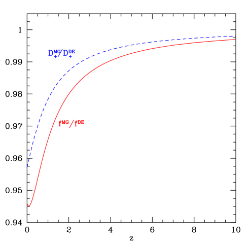
FIG. 1.: Growth of perturbations as a function of redshift in dark energy (DE) models and modified gravity (MG) models with identical expansion histories, given by Eq. (35). The dashed line shows the ratio of density perturbation growth factors $D_{+}^{\rm MG}/D_{+}^{\rm DE}$, the solid line shows the ratio of the velocity perturbation growth factors $f^{\rm MG}/f^{\rm DE}$.

Let us now consider how the linear growth of perturbations can distinguish between dark energy and modified gravity models with the same expansion history. This is relevant because in the near future, planned experiments will measure the expansion history from $z=0$ to $z\simeq 2$ with very good accuracy (see e.g. [24, 25]). For other tests of gravity using large-scale structure see e.g. [26, 27]. To illustrate our results, we assume a modified Friedman equation given by

$$g(x)=\Big{[}c+\sqrt{c^{2}+x}\Big{]}^{2},$$ (35)

where $c$ is a constant, $a=(1-\Omega_{m})/2$. This corresponds to “extra-dimensions-inspired” modified gravity in [20] when their $\alpha=1$ (which corresponds to an effective equation of state with $w_{\rm eff}\simeq-0.7$ for $z$ between 0 and 2). In all calculations we set $\Omega_{m}=1/3$ for simplicity.

Figure 1 shows the results for the ratio $D_{+}^{\rm MG}/D_{+}^{\rm DE}$ (dashed line) as a function of redshift $z$. The modified gravity perturbations growth slower, and the decline of this ratio as redshift approaches zero is a general feature, not restricted to Eq. (35), that can be understood in general terms. From Eqs. (31-33) we see that for the same expansion history, the difference in growth can be thought as coming from an effective gravitational constant $G[g^{\prime}(\bar{x})+3\bar{x}g^{\prime\prime}(\bar{x})]$. At high redshift $g(\bar{x})\approx\bar{x}$, but at low redshift the constraint that the universe accelerates ($\ddot{\bar{a}}>0$) implies ${\rm d}\ln g/{\rm d}\ln\bar{x}<2/3$. If we model $g(x)$ as a local power-law, $g(\bar{x})\sim\bar{x}^{n}$, where $n$ changes very slowly from $n=1$ at high redshift to $n<2/3$ when $z\sim 1$, we see that $g^{\prime}(\bar{x})+3\bar{x}g^{\prime\prime}(\bar{x})\sim n(3n-2)g(\bar{x})/\bar{x}$, so as $n$ becomes closer to $2/3$, $g^{\prime}(\bar{x})+3\bar{x}g^{\prime\prime}(\bar{x})$ becomes small. Although in practice one must take into account the time dependence of $n$, this illustrates why the growth of structure is slower in the case of modified gravity. As long as we are only concerned with linear perturbations around a cosmological background, this effective Newton’s constant is wavelength independent. However, when perturbations become strong, and self-gravitation dominates cosmology, we will see that the effective $G$ does acquire distance dependence (see Sec. VI).

Figure 1 also shows the ratio $f^{\rm MG}/f^{\rm DE}$, where $f\equiv{\rm d}\ln D_{+}/{\rm d}\ln\bar{a}$ governs the growth of velocity fluctuations in linear perturbation theory, that is, the velocity divergence evolves as $\theta=-\bar{H}\bar{a}f\delta$ from the linearized continuity equation (see e.g., Ref. [21]). We see that slower growth leads to smaller time derivative, thus $f^{\rm MG}/f^{\rm DE}$ also decreases as $z\rightarrow 0$. These deviations are detectable with precision measures of large-scale structure; for example, $D_{+}$ and $f$ can be derived from joint measurements of the redshift-space power spectrum anisotropy and bispectrum. The Sloan Digital Sky Survey should be able to probe these quantities with statistical errors of order a few percent [28].

So far we have discussed the linear growth of perturbations. Equation (30) can be recast in a more useful way to study the non-linear evolution in perturbation theory,

$$3\bar{x}g(\bar{x}){d^{2}\delta\over d\bar{x}^{2}}+\left[g(\bar{x})+{3\over 2}\bar{x}g^{\prime}(\bar{x})\right]{d\delta\over d\bar{x}}-4\frac{\bar{x}g(\bar{x})}{1+\delta}\Big{(}\frac{d\delta}{d\bar{x}}\Big{)}^{2} = \Big{(}\frac{1+\delta}{2x}\Big{)}\ \sum_{n=1}^{\infty}\frac{(\delta\bar{x})^{n}}{n!}$$ (37)

$$\times\Big{[}(3n-2)g^{(n)}+3\bar{x}g^{(n+1)}\Big{]}$$

A couple of points are worth stressing here. First, this equation becomes identical to that in the standard dark energy scenario, Eq. (26), only if $g(x)=A_{1}+x$, i.e. a curvature term is no longer degenerate as in the linear case. Expanded to second order, this equation can be used to compute the skewness of the density field (see also [22]); we have checked that for the same expansion history given by Eq. (35) the skewness changes by less than one percent in modified gravity compared to dark energy models. Only a rather large third derivative of $g$ can induce an appreciable change in skewness from that in the dark energy case. Such extreme models have been studied in [22] (e.g. using Eq. (55) below with $n=0$ and $q=5$); we have verified that in this case the skewness can change by up to $10\%$ compared to dark energy models, and also $D_{+}^{\rm MG}/D_{+}^{\rm DE}$ can be larger than unity (up to $1.2$ at $z=0$) due to a fast variation of $g$ with $\bar{x}$.

Ultimately, unless the source of acceleration is a vacuum energy component, determination of the expansion history of the universe plus the growth of structure should allow us to identify, through the divergence between Eq. (26) and Eq. (30), whether today’s cosmic acceleration may be attributed to modified gravity or dark energy.

V Evolution of Gravitational Potentials: The ISW Effect

The microwave background provides another window to differentiate between dark energy and modified gravity through the late-time integrated Sachs-Wolfe (ISW) effect due to the decay in gravitational potentials at late times (see e.g. [29]). In order to assess how a modified gravitational force law affects the ISW effect, we must find the evolution of the cosmological gravitational potentials, $\Psi(t,\lambda)$ and $\Phi(t,\lambda)$, which are defined using the line element

$$ds^{2}=\left[1+2\Psi(t,\lambda)\right]dt^{2}-\bar{a}^{2}(t)\left[1+2\Phi(t,\lambda)\right]\left[d\lambda^{2}+\lambda^{2}d\Omega\right]\ ,$$ (38)

where $\bar{a}(t)$ is the background scale factor evolution. We are only interested in potentials and overdensities that are small and, therefore, only interested in linear perturbations around the cosmological background.

We have the equations for the evolution of a linear top-hat overdensity $\delta(t)$ of radial extent $\lambda_{*}$, Eq. (32), and we know the complete metric for that matter configuration:

$$ds^{2}=dt^{2}-\bar{a}^{2}(t)\left[{d\lambda^{2}\over 1-\kappa\lambda^{2}}+\lambda^{2}d\Omega\right]\ ,$$ (39)

where $a^{3}=(1+\delta)\bar{a}^{3}$, and $\kappa$ is the curvature parameter associated with the magnitude of the overdensity. Using $r=a\lambda_{*}$ and integrating Eq. (27), we arrive at

$$\dot{r}^{2}=(1-\kappa\lambda_{*}^{2})-g_{rr}^{-1}\ ,$$ (40)

where the constant of integration is determined by smoothly connecting a background cosmological expansion outside $\lambda_{*}$ with an overdense space inside $\lambda_{*}$. Then, one may deduce that

$$\kappa=\bar{a}^{2}H_{0}^{2}\bar{x}g^{\prime}(\bar{x})\delta+{2\over 3}\bar{a}\dot{\bar{a}}\dot{\delta}\ .$$ (41)

One can confirm using Eq. (34) that $\kappa$ is indeed a constant.

One needs only identify a coordinate transformation taking the metric Eq. (39) into the form Eq. (38) and read off $\Psi$ and $\Phi$. After some algebra we find

$$\Psi(t,\lambda) = -{\bar{a}^{2}\lambda_{*}^{2}\over 6}\left(1-{\lambda^{2}\over\lambda_{*}^{2}}\right)\left[4\pi G\bar{\rho}\delta(g^{\prime}+3\bar{x}g^{\prime\prime})\right]$$ (42)

$$\Phi(t,\lambda) = {\bar{a}^{2}\lambda_{*}^{2}\over 6}\left(1-{\lambda^{2}\over\lambda_{*}^{2}}\right)\left[4\pi G\bar{\rho}\delta g^{\prime}\right]\ ,$$ (43)

when $\lambda<\lambda_{*}$ and the potentials vanish outside $\lambda_{*}$. By superposing top-hat linear overdensities, we surmise that for general $r$–dependent $\delta$

$$\nabla^{2}\Psi = 4\pi G\bar{\rho}\bar{a}^{2}\left[g^{\prime}(\bar{x})+3\bar{x}g^{\prime\prime}(\bar{x})\right]\delta$$ (44)

$$\nabla^{2}\Phi = -4\pi G\bar{\rho}\bar{a}^{2}g^{\prime}(\bar{x})\delta\ ,$$ (45)

where the Laplacian is with respect to comoving coordinates. These expressions for the linear gravitational potentials are the generalization of the usual result for Einstein gravity, around a specific cosmological background. One arrives at time-dependent effective Newton’s constants (in general, different for $\Psi$ versus $\Phi$). At early times, $G_{\rm eff}\rightarrow G$ but deviates from the true Newton’s constant significantly as $\bar{H}\rightarrow H_{0}$. Note that this large discrepancy only applies to self-gravitation of linear density perturbations. For example, solar system manifestations of Newton’s constant, in this context, are not linear and will only have small deviations from the true Newton’s constant, as will be seen in the next section.

We may now take Eqs. (45–44) and apply them to ascertain the ISW effect on the cosmic microwave background, which is proportional to the integral of $\dot{\Phi}-\dot{\Psi}$ along the line of sight  (see e.g. [29]). From Eqs. (44–45) we find, after a Fourier transformation,

$$A(\dot{\Phi}-\dot{\Psi})^{\rm DE} = (1-f^{\rm DE})\ D_{+}^{\rm DE}$$ (46)

$$A(\dot{\Phi}-\dot{\Psi})^{\rm MG} = \Big{[}(1-f^{\rm MG})(g^{\prime}+\frac{3}{2}\bar{x}g^{\prime\prime})+\frac{3}{2}(5\bar{x}g^{\prime\prime}+3\bar{x}^{2}g^{\prime\prime\prime})\Big{]}\ D_{+}^{\rm MG}\ ,$$ (47)

where $A\equiv-k^{2}/(8\pi G\bar{H}\bar{\rho}\bar{a}^{2}\delta_{0})$ with $k$ the comoving wavenumber and $\delta_{0}$ the amplitude of density perturbations at some early time. The second term in Eq. (47), representing the time derivative of the effective gravitational constant, leads to an additional decay of the potentials that can be quite significant at low redshifts.

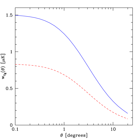
FIG. 2.: The angular cross-correlation function between galaxies and CMB temperature anisotropies. The solid line shows the dark energy case, dashed line corresponds to modified gravity with the same expansion history.

We compute the cross-correlation between temperature anisotropies due to the ISW effect and galaxy fluctuations, which has recently been detected using the WMAP and SDSS datasets [30, 31]. The angular cross-correlation function $w_{Tg}(\theta)$ can be written as

$$w^{\rm DE}_{Tg}(\theta)=3T_{0}\Omega_{m}b(2\pi)^{2}\frac{H_{0}^{3}}{c^{3}}\int dz\sqrt{g}\ D_{+}^{2}(1-f)\ w_{g}(z)\int\frac{dk}{k}P(k)J_{0}(k\theta\chi)\ ,$$ (48)

for the dark energy case, whereas for modified gravity

$$w^{\rm MG}_{Tg}(\theta) = 3T_{0}\Omega_{m}b(2\pi)^{2}\frac{H_{0}^{3}}{c^{3}}\int dz\sqrt{g}\ D_{+}^{2}\Big{[}(1-f)(g^{\prime}+\frac{3}{2}\bar{x}g^{\prime\prime})+\frac{3}{2}\bar{x}(5g^{\prime\prime}+3\bar{x}g^{\prime\prime\prime})\Big{]}\ w_{g}(z)$$ (50)

$$\times\int\frac{dk}{k}P(k)J_{0}(k\theta\chi)\ ,$$

where we have assumed the small-angle approximation, and $T_{0}$ is the CMB temperature, $b$ is the linear bias of LRG galaxies, $w_{g}(z)$ is the galaxy selection function, $P(k)$ is the dark matter power spectrum at $z=0$, $J_{0}$ is a Bessel function, and $\chi(z)$ is the comoving distance as a function of redshift $z$. We assume, following the results in [31] (see their Fig. 3), that $b=5.47$, and use their selection function for the $z=0.49$ sample.

Figure 2 shows the results, again using the expansion history given by Eq. (35). We see that the MG angular correlation function is suppressed by a factor of about two compared to the case of DE, for the same expansion history. This anomaly is a reflection of the order-unity anomalous effective Newton’s constant seen in Eqs. (45–44) when the Hubble parameter is near today’s value. Although the ISW anomaly is not yet detectable, it should be so in the near future with the completion of the SDSS survey or other future probes of structure at intermediate redshifts.

The suppression of the late-time ISW effect that results from MG can help explain, at least partially, the low amplitude of the CMB power spectrum at low multipoles as confirmed by WMAP [32]. It is worth emphasizing that these results depend on the specific prescription of exploiting Birkhoff’s law for understanding modified gravity from cosmological physics, and it will be important to check whether the large ISW discrepancy carries over to more general prescriptions of modified gravity.

VI Orbit Precession

We have seen that modification of the Friedmann equation leads to a modification of the gravitational force law. This modification of the force law may, in turn, lead to small-but-detectable corrections at distances much smaller than today’s Hubble scale. Indeed, under some circumstances (e.g., if no physics other than that deduced from cosmological evolution emerges at small scales) these alterations of cosmology on the largest observable distances may cause observable deviations from known physics at even solar system scales. Let us elaborate.

The precession $\Delta\phi$ of the perihelion per orbit in the background of a metric of the form Eq. (4) may be determined in the usual way:

$$\Delta\phi=\int dr{J\over r^{2}}\sqrt{g_{00}g_{rr}\over E^{2}-g_{00}(1+J/r^{2})}\ ,$$ (51)

where $E=N^{2}\dot{T}$, $J=r^{2}\dot{\phi}$, and dot refers to differentiation with respect to proper time. For a nearly circular orbit with a metric of the form Eq. (24), one may compute the precession rate:

$${d\over dT}\Delta\phi={H_{0}\over\sqrt{2}}x^{1/2}\left[\sqrt{g-{3\over 2}xg^{\prime}\over 4g-{9\over 2}xg^{\prime}+{9\over 2}x^{2}g^{\prime\prime}}-1\right]\ ,$$ (52)

with again, $x={r_{*}^{3}\over r^{3}}$. The leading contribution to orbit precession from the altered metric Eq. (24) comes from the simple alteration of the Newtonian potential.

We are particularly interested in orbits whose radii around a central body of Schwarzschild radius $r_{g}$ are much smaller than $r_{*}=(r_{g}/H_{0}^{2})^{1/3}$. Then, corrections from the modified gravity are small. One may represent the function $g(x)$ as

$$g(x)=x\left[1+\delta g(x)\right],$$ (53)

with $\delta g(x)\ll{\cal O}(1)$. Then, Eq. (52) reduces to

$${d\over dT}\Delta\phi={6H_{0}\over\sqrt{2}}x^{3/2}\left(\delta g^{\prime}+{3x\over 4}\delta g^{\prime\prime}\right)\ ,$$ (54)

to leading order in $\delta g$. Recall that here $x\gg 1$.

Take as an instructive example the form of the modified Friedmann equation found in Cardassian models [19]. This can be written as

$$g(x)=x\left[1+cx^{-q(1-n)}\right]^{1/q}\ ,$$ (55)

where $n$ and $q$ are parameters of the modification and where

$$c=\left({(1+z_{\rm eq})^{3q}\over 1+(1+z_{\rm eq})^{3q(1-n)}}\right)^{1-n}\ .$$ (56)

The quantity $z_{\rm eq}$ is the redshift at which the two terms inside bracket in Eq. (55) are equal, a quantity of order unity. Then, using Eq. (54), the anomalous orbit precession rate is

$${d\over dT}\Delta\phi={3cH_{0}\over 2\sqrt{2}}(n-1)[3q(n-1)+1]\left({r^{3}\over r_{*}^{3}}\right)^{q(1-n)-{1\over 2}}\ .$$ (57)

When $q(1-n)={1\over 2}$, this expression is independent of the radius of the orbit, or the mass of the central body, and the anomalous precession rate is proportional to today’s Hubble parameter, $H_{0}\sim 10~{}\mu{\rm as/year}$. Such a precession rate is on the threshold of detection by precision ephemeris measurements of the inner solar system, particularly with intriguing developments this decade coming from two Mercury-bound missions (BepiColombo and MESSENGER) as well as improvements in lunar ranging observations [14, 15, 33, 34, 35, 36]. When $q(1-n)\neq{1\over 2}$, there is a relevant distance-dependence for the anomalous precession rate, where the governing length scale is once again $r_{*}$. Since we are primarily concerned with orbits such that $r\ll r_{*}$, the dimensionless distance factor in the anomalous precession rate, $(r^{3}/r_{*}^{3})^{q(1-n)-{1\over 2}}$, will either be huge or tiny. Thus, with solar system constraints in mind, the parametric range where $q(1-n)\lesssim{1\over 2}$ can already be ruled out. However, for $q(1-n)\gg{1\over 2}$, no solar system test are likely to discover discrepancies based on anomalous orbit precession in the foreseeable future.

VII Concluding Remarks

In this paper we showed how modifying gravity to effect the observed late-time cosmological acceleration at scales of today’s Hubble radius, $H_{0}^{-1}$, can lead naturally to corresponding modifications of gravitational interactions at scales much shorter than $H_{0}^{-1}$. Indeed, by presuming that the new gravitational physics obeys a limited version of Birkhoff’s law, we were able to derive the precise form of the modifications to Newton’s law of gravitation at short (sub-cosmological) distances. We then showed that an observer in the gravitational field of a central source whose Schwarzschild radius is $r_{g}$, experiences substantial deviations from the usual Schwarzschild metric at all distances greater than approximately

$$r_{*}=\left({r_{g}\over H_{0}^{2}}\right)^{1/3}\ .$$ (58)

For many models these deviations will be measurable through observation of orbital precession of solar system objects in the coming decade. We also discussed the evolution of density perturbations and showed that, unless the acceleration of the universe is driven by an effective vacuum energy, simultaneous measurement of the expansion history and growth of large-scale structure can be used to distinguish modified gravity from dark energy. In addition, the cross-correlation of galaxy distribution and the cosmic microwave background temperature anisotropy can detect anomalies in the late-time integrated Sachs–Wolfe effect caused by modified gravity. Such measurements will be available imminently.

It is instructive that these results are identical to those found for the braneworld theory of Dvali, Gabadadze, and Porrati (DGP), even though DGP gravity does not respect any dynamical version of Birkhoff’s law. The correspondence between the scales of departure from Einstein gravity in DGP and the Birkhoff’s Law theories seems not to be a coincidence. Indeed, one suspects that it is quite general. Imagine cosmology at extremely late times, when all matter surrounding a particular gravitational source is swept away. Then, if one believes that an isolated, central source has a (quasi)static metric description, it should be Schwarzschild at short distances and deviate from Schwarzschild at large-enough distances. How large? Since this metric must still encode the cosmology within it, i.e., test observers at large distances from the source should recede from the source in the manner dictated by the given late-time (accelerating) cosmology, the empty space metric must include a repulsive force at distances where cosmological flow overcomes the local gravitational binding of the central source. Thus, we expect substantial deviations from Schwarzschild (in the form of a repulsive force) at distances ${\cal O}(r_{*})$, Thus, it is not unreasonable to expect general modifications of cosmology at today’s Hubble scale to inevitably affect local gravitational interactions at distances governed by $r_{*}$; it is only the precise functional form of the deviations that will vary from model to model.

- [1] S. Perlmutter et al. [Supernova Cosmology Project Collaboration], Astrophys. J. 517, 565 (1999).
- [2] A. G. Riess et al. [Supernova Search Team Collaboration], Astron. J. 116, 1009 (1998).
- [3] M. Milgrom, Astrophys. J. 270, 365 (1983).
- [4] R. H. Sanders and S. S. McGaugh, Annual Review of Astronomy and Astrophysics Sep 2002, Vol. 40: 263-317 [arXiv:astro-ph/0204521].
- [5] G. Dvali, G. Gabadadze and M. Porrati, Phys. Lett. B 485, 208 (2000).
- [6] G. R. Dvali, G. Gabadadze, M. Kolanovic and F. Nitti, Phys. Rev. D 64, 084004 (2001).
- [7] G. R. Dvali, G. Gabadadze, M. Kolanovic and F. Nitti, Phys. Rev. D 65, 024031 (2002).
- [8] C. Deffayet, Phys. Lett. B 502, 199 (2001).
- [9] C. Deffayet, G. R. Dvali and G. Gabadadze, Phys. Rev. D 65, 044023 (2002).
- [10] C. Deffayet, G. R. Dvali, G. Gabadadze and A. I. Vainshtein, Phys. Rev. D 65, 044026 (2002).
- [11] A. Lue, Phys. Rev. D 66, 043509 (2002).
- [12] A. Gruzinov, arXiv:astro-ph/0112246.
- [13] M. Porrati, Phys. Lett. B 534, 209 (2002).
- [14] A. Lue and G. Starkman, Phys. Rev. D 67, 064002 (2003).
- [15] G. Dvali, A. Gruzinov and M. Zaldarriaga, arXiv:hep-ph/0212069.
- [16] T. Damour, I. I. Kogan and A. Papazoglou, Phys. Rev. D 66, 104025 (2002).
- [17] S. M. Carroll, V. Duvvuri, M. Trodden and M. S. Turner, arXiv:astro-ph/0306438.
- [18] K. Freese and M. Lewis, Phys. Lett. B 540, 1 (2002).
- [19] K. Freese, arXiv:hep-ph/0208264.
- [20] G. Dvali and M. S. Turner, arXiv:astro-ph/0301510.
- [21] P. J. E. Peebles, Principles of Physical Cosmology, Princeton, 1993.
- [22] T. Multamaki, E. Gaztañaga and M. Manera, arXiv:astro-ph/0303526.
- [23] D. Heath, MNRAS 152, 75 (1977)
- [24] J. A. Frieman, D. Huterer, E. V. Linder, M. S. Turner, Phys. Rev. D 67, 083505 (2003).
- [25] K. Benabed and L. Van Waerbeke, arXiv:astro-ph/0306033.
- [26] J-P. Uzan and F. Bernardeau, Phys. Rev. D 64, 083004 (2001).
- [27] E. Gaztañaga and J. A. Lobo, Ap. J. 548, 47 (2001).
- [28] S. Colombi, I. Szapudi, and A. S. Szalay, MNRAS 296, 253 (1998)
- [29] W. Hu, and S. Dodelson, ARA&A, 40, 171 (2002)
- [30] P. Fosalba, E. Gaztañaga, and F. J. Castander, arXiv:astro-ph/0307249.
- [31] R. Scranton et al., arXiv:astro-ph/0307335.
- [32] D. N. Spergel et al., arXiv:astro-ph/0302209
- [33] K. Nordtvedt, Phys. Rev. D 61, 122001 (2000).
- [34] J. G. Williams, X. X. Newhall and J. O. Dickey, Phys. Rev. D 53, 6730 (1996).
- [35] A. Milani, D. Vokrouhlicky, D. Villani, C. Bonanno and A. Rossi, Phys. Rev. D 66, 082001 (2002).
- [36] C. M. Will, Living Rev. Rel. 4, 4 (2001) [arXiv:gr-qc/0103036].