Observational constraints on braneworld chaotic inflation

Abstract

We examine observational constraints on chaotic inflation models in the Randall–Sundrum Type II braneworld. If inflation takes place in the high-energy regime, the perturbations produced by the quadratic potential are further from scale-invariance than in the standard cosmology, in the quartic case more or less unchanged, while for potentials of greater exponent the trend is reversed. We test these predictions against a data compilation including the Wilkinson Microwave Anisotropy Probe measurements of microwave anisotropies and the 2dF galaxy power spectrum. While in the standard cosmology the quartic potential is at the border of what the data allow and all higher powers excluded, we find that in the high-energy regime of braneworld inflation even the quadratic case is under strong observational pressure. We also investigate the intermediate regime where the brane tension is comparable to the inflationary energy scale, where the deviations from scale-invariance prove to be greater.

I Introduction

Braneworld cosmology has opened up a possible new phenomenology for the cosmology of the early Universe. Amongst the ideas presently under investigation, which are nicely reviewed in Ref. revs , are the ekpyrotic and cyclic universes ekpy , where the Big Bang may be due to a collision of branes, and various incarnations of braneworld inflation, where the scalar field may be associated with the distance between branes radion , or may be a bulk field bulk , or may live on the brane MWBH . In this paper we explore the simplest and most conservative scenario, based on the Randall–Sundrum Type II model RSII where there is a single brane upon which the inflaton lives. In this scenario the detailed form of the perturbations produced by a given inflationary potential is modified because the Friedmann equation is modified at high energy, and because the gravitational wave perturbations are able to penetrate the bulk dimension.

Recently, driven by the announcement of first results from the Wilkinson Microwave Anisotropy Probe (WMAP) satellite wmap , the global cosmological data set has reached a level where it is able to significantly constrain inflationary models based on the predicted perturbations. Our aim in this short paper is to capitalize on this by obtaining observational constraints on some simple braneworld inflation models. We use the recently-published constraints of Leach and Liddle LLnew , who used a compilation of microwave anisotropy data plus the 2dF galaxy power spectrum to obtain constraints on the inflationary slow-roll parameters. These results are directly applicable also to the braneworld case and so we do not need to repeat a data analysis process.

II Basic formulae

We follow the notation set down by Liddle and Taylor LT . In the Randall–Sundrum Type II model RSII the Friedmann equation receives an additional term quadratic in the density HE . The Hubble parameter $H$ is related to the energy density $\rho$ by

$$H^{2}=\frac{8\pi}{3M_{4}^{2}}\,\rho\,\left(1+\frac{\rho}{2\lambda}\right)\,,$$ (1)

where $M_{4}$ is the four-dimensional Planck mass and $\lambda$ is the brane tension. We have set the four-dimensional cosmological constant to zero, and assumed that inflation rapidly makes any dark radiation term negligible. This reduces to the usual Friedmann equation for $\rho\ll\lambda$. If the Universe is dominated by a scalar field $\phi$ with potential $V(\phi)$, we can use the slow-roll approximation to write this as

$$H^{2}\simeq\frac{8\pi}{3M_{4}^{2}}\,V\,\left(1+\frac{V}{2\lambda}\right)\,.$$ (2)

The scalar field obeys the usual slow-roll equation

$$3H\dot{\phi}\simeq-V^{\prime}\,,$$ (3)

where prime indicates derivative with respect to $\phi$, and dot a derivative with respect to time. The amount of expansion, in terms of $e$-foldings, is given by MWBH

$$N\simeq-\frac{8\pi}{M_{4}^{2}}\int^{\phi_{\rm f}}_{\phi_{\rm i}}\frac{V}{V^{\prime}}\left(1+\frac{V}{2\lambda}\right)d\phi\,,$$ (4)

where $\phi_{\rm i}$ and $\phi_{\rm f}$ are the values of the scalar field at the beginning and end of the expansion respectively.

Using the slow-roll approximation as formulated by Maartens et al. MWBH , the spectra of scalar MWBH and tensor LMW ; HL perturbations are given by

$$A_{{\rm S}}^{2} = \frac{4}{25}\,\frac{H^{2}}{\dot{\phi}^{2}}\,\left(\frac{H}{2\pi}\right)^{2}\simeq\frac{512\pi}{75M_{4}^{6}}\,\frac{V^{3}}{V^{\prime 2}}\,\left(1+\frac{V}{2\lambda}\right)^{3}\,;$$ (5)

$$A_{{\rm T}}^{2} = \frac{4}{25\pi}\,\frac{H^{2}}{M_{4}^{2}}\,F^{2}(H/\mu)\,,$$ (6)

where

$$F(x) = \left[\sqrt{1+x^{2}}-x^{2}\ln\left(\frac{1}{x}+\sqrt{1+\frac{1}{x^{2}}}\right)\right]^{-1/2}\,,$$ (7)

$$= \left[\sqrt{1+x^{2}}-x^{2}\sinh^{-1}\frac{1}{x}\right]^{-1/2}\,,$$

and the mass scale $\mu$ is given by

$$\mu=\sqrt{\frac{4\pi}{3}}\,\sqrt{\lambda}\,\frac{1}{M_{4}}\,.$$ (8)

The expressions for the spectra are, as always, to be evaluated at Hubble radius crossing $k=aH$, and the spectral indices of the scalars and tensors are defined as usual by

$$n-1\equiv\frac{d\ln A_{{\rm S}}^{2}}{d\ln k}\quad;\quad n_{{\rm T}}\equiv\frac{d\ln A_{{\rm T}}^{2}}{d\ln k}\,.$$ (9)

If one defines slow-roll parameters, generalizing the usual ones, by MWBH

$$\epsilon_{{\rm B}} \equiv \frac{M_{4}^{2}}{16\pi}\,\left(\frac{V^{\prime}}{V}\right)^{2}\;\frac{1+V/\lambda}{\left(1+V/2\lambda\right)^{2}}\,;$$ (10)

$$\eta_{{\rm B}} \equiv \frac{M_{4}^{2}}{8\pi}\,\frac{V^{\prime\prime}}{V}\;\frac{1}{1+V/2\lambda}\,,$$ (11)

then the scalar spectral index, in the slow-roll approximation, obeys the usual equation

$$n-1\simeq-6\epsilon_{{\rm B}}+2\eta_{{\rm B}}\,.$$ (12)

We define the ratio of tensor to scalar perturbations as

$$R\equiv 16\,\frac{A_{{\rm T}}^{2}}{A_{{\rm S}}^{2}}\,,$$ (13)

which means our definition of $R$ matches that of Ref. LLnew , with $R\simeq 16\epsilon_{{\rm B}}$ in the low-energy limit (note however that that paper also defines a slightly different quantity $R_{10}$).

III Model predictions

We restrict our discussion to potentials of the form

$$V=m\phi^{\alpha}\,,$$ (14)

where normally $\alpha$ is an even integer, and $m$ is a constant. This includes the popular quadratic and quartic potentials, which we will explore in particular detail.

In the standard cosmology, the requirement that the perturbations have the observed amplitude fixes the normalization $m$ of the potential. However, in the braneworld we additionally have the brane tension $\lambda$. We proceed by taking $\lambda$ as a free parameter to be varied, and then adjust the normalization of the potential to obtain the correct amplitude of perturbations for that $\lambda$. This fixes the inflationary energy scale, whose relation to the chosen value of $\lambda$ then determines whether we are in the high- or low-energy regime.

With a potential of the above form, setting $\alpha\geq 2$, the slow-roll parameters are found to satisfy

$$\frac{1}{2}\eta_{\rm B}\leq\epsilon_{\rm B}\leq 2\eta_{\rm B}\,,$$ (15)

for any value of $\lambda$. Inflation ends when the slow-roll conditions, $\epsilon_{\rm B}\ll 1$ and $|\eta_{\rm B}|\ll 1$, are violated. For ease of computation, we take $\eta_{\rm B}=1$ to be the condition for the end of inflation, though it would make no significant difference had we adopted the usual $\epsilon_{\rm B}=1$

The equations simplify significantly in the high- and low-energy limits, in which we may obtain expressions for $n$ and $R$ which are independent of $\lambda$ and $m$:

$$n_{{\rm low}}-1 = -\frac{\alpha+2}{2N-1+\alpha}\,;$$ (16)

$$n_{{\rm high}}-1 = -\frac{4\alpha+2}{(2+\alpha)N-1+\alpha}\,;$$ (17)

$$R_{{\rm low}} = \frac{8\alpha}{2N-1+\alpha}\,;$$ (18)

$$R_{{\rm high}} = \frac{24\alpha}{(2+\alpha)N-1+\alpha}\,.$$ (19)

In the limit as $\alpha$ tends to infinity, in the high-energy regime the scalar spectral index tends to

$$n_{{\rm high}}-1=\frac{4}{N+1}\,,$$ (20)

which corresponds to steep inflation driven by an exponential potential CLL . Table 1 shows some values for particular models.

Table 1: low- and high-energy limits for scalar spectral index, $n$, and ratio of tensor to scalar perturbations, $R$, for potentials of the form $V\propto\phi^{\alpha}$. The end of inflation is defined by $\eta_{\rm B}=1$ and the number of $e$-foldings is taken to be 55.

$$\begin{array}[]{c | c c c c}\alpha&n_{\mathrm{low}}-1&n_{\mathrm{high}}-1&R_{\mathrm{low}}&R_{\mathrm{high}}\\ \hline\cr 2&-0.036&-0.045&0.144&0.217\\ 4&-0.053&-0.054&0.283&0.288\\ 6&-0.070&-0.058&0.417&0.324\\ 8&-0.085&-0.061&0.547&0.345\end{array}$$

In all the following, we assume that the number of $e$-foldings before the end of inflation at which observable perturbations are generated corresponds to $N=55$ DH ; LLe . The observational values we will use are defined at about 4 $e$-foldings within the present Hubble radius LLnew . One might have thought that the number 55 ought to be significantly modified in the case of low $\lambda$ because then the reheating and radiation eras would at least partly take place in the high-energy regime, giving a different expansion law. However the main quantity entering the calculation is the density as a function of scale factor, rather than of time, which is unchanged, and we find it is a good approximation to take the number of $e$-foldings as independent of the brane tension.

In their paper describing the slow-roll formalism for braneworld models, Maartens et al. MWBH noted that braneworld corrections tend to drive models towards scale-invariance (i.e. smaller values of $R$ and $|n-1|$). While this is true at a given location on the potential, there is a competing effect that the location of the potential corresponding to observable perturbations will be closer to the minimum of the potential, due to the extra friction from the braneworld term in the Friedmann equation. The above results show that for small $\alpha$ this latter effect dominates, moving us away from scale-invariance, whereas for large $\alpha$ it is the former effect which dominates.

Figure 1: Theoretical predictions for $n-1$ and $R$ against $\lambda$ for quadratic and quartic potentials. The models are all normalized to give the correct perturbation amplitude, and $M_{4}$ has been set to be equal to 1.

For quadratic and quartic potentials, we have obtained $n$ and $R$ as functions of the brane tension $\lambda$. This is done firstly by finding the value of the scalar field at the end of inflation, in terms of $m$ and $\lambda$, by solving $\eta_{\rm B}=1$ for $\phi$. Using this, Eq. (4) for $N$ can be solved to give $\phi_{55}(m,\lambda)$, where $\phi_{55}$ is the value of the scalar field 55 $e$-foldings before the end of inflation. Finally, the COBE normalization is imposed, in the form $A_{\rm S}=2\times 10^{-5}$ BLW . Eq. (5) for $A_{\rm S}^{2}$, which is evaluated at $\phi=\phi_{55}$, can then be solved numerically to give $m(\lambda)$. This leaves $\lambda$ as the only free parameter when determining the predicted perturbations.

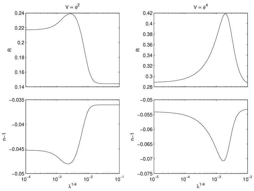
Fig. 1 shows the results for the quadratic and quartic potentials. Large and small values of $\lambda$ correspond to the low- and high-energy regimes respectively, with asymptotic values for $n$ and $R$ matching the analytic expressions Eqs. (16)–(19). In between there is a continuous curve interpolating between the regimes. However note that the interpolation is not monotonic; in fact the intermediate regime features greater departures from scale-invariance than either of the limits.

IV Comparison with observations

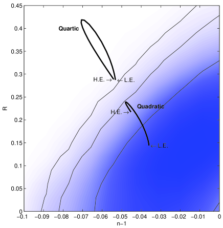
Having made predictions for $n$ and $R$, we are able to compare with observational data directly using the recent analysis of Leach and Liddle LLnew , who used a compilation of microwave anisotropy data including WMAP, plus the 2dF galaxy power spectrum, to constrain these parameters. Having fixed the number of $e$-foldings of inflation to 55, a given model lives at a location in the $n$–$R$ plane, and as $\lambda$ is varied it traces out a trajectory in that plane interpolating between low-energy and high-energy values. In reality, the points should be somewhat blurred to allow for the uncertainty in determining $N$ LLe .

Figure 2: Theoretical predictions compared to observational constraints for the quadratic and quartic potentials, as a function of the brane tension $\lambda$. The low- and high-energy limits are shown. The observational contours are one-, two- and three-sigma confidence levels.

In Fig. 2 we show the results for the quadratic and quartic potentials. The endpoints of the two curves correspond to the low- and high-energy limits described in the previous section, and the curves the interpolation between them. For these potentials, we see that the braneworld moves us further from scale-invariance, an effect which can be particularly prominent when the brane tension is comparable to the inflationary energy scale.

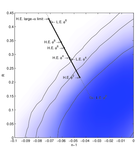
Fig. 3 shows the low- and high-energy limits as a function of exponent $\alpha$, beginning at $\alpha=2$. We see that the perturbations are much more sensitive to $\alpha$ in the low-energy limit than in the high-energy limit, and indeed once $\alpha$ exceeds four it is the high-energy limit which is closer to scale-invariance. However by this time the models have already moved into the observationally excluded region. We therefore conclude that the observational upper limit on $\alpha$ is stronger in the braneworld scenario than in the standard cosmology, though with present observations the constraint in each case lies between $\alpha=2$ and $4$, precisely where depending on how strict an exclusion limit one demands. The quartic potential is however much more strongly excluded in the intermediate regime than in either of the limits.

Figure 3: As Fig. 2, but now showing the low-energy limit (dotted line) and high-energy limit (solid line) as a function of $\alpha$, for $\alpha\geq 2$. We highlight the locations corresponding to $\alpha$ being an even integer, and the large-$\alpha$ limit in the high-energy case.

Note that the original steep inflation model with an exponential potential CLL gives the same perturbations as in the high-energy large-$\alpha$ limit. It is therefore comfortably ruled out by the data, though steep inflation may still be viable with curvaton reheating LU .

V Summary

In this paper we have computed the perturbation spectra for a set of simple braneworld inflation models with monomial potentials, and confronted them with the current observational dataset. While naïve expectation might have been that the braneworld models gave spectra closer to scale-invariance (as preferred by the data), we have found that for small exponents the perturbations are further from scale-invariance. Accordingly, observational constraints on the exponent are strengthened in the braneworld scenario. While the quadratic potential is still allowed at two-sigma for any value of the brane tension, the quartic potential is under strong observational pressure, particularly in the case where the inflationary energy scale is close to the brane tension.

References

- (1) F. Quevedo, Class. Quant. Grav. 19, 5721 (2002), hep-th/0210292; P. Brax and C. van de Bruck, hep-th/0303095.
- (2) J. Khoury, B. A. Ovrut, P. J. Steinhardt, and N. Turok, Phys. Rev. D64, 123522 (2001), hep-th/0103239; P. J. Steinhardt and N. Turok, Phys. Rev. D65 126003 (2002), hep-th/0111098.
- (3) G. Dvali and S.-H. H. Tye, Phys. Lett. B450, 72 (1999), hep-ph/9812483; A. Mazumdar and A. Pérez-Lorenzana, Phys. Lett. B508, 340 (2001), hep-ph/0102174.
- (4) H. A. Chamblin and H. S. Reall, Nucl. Phys. B562, 133 (1999), hep-th/9903225; R. N. Mohapatra, A. Pérez-Lorenzana, and C. A. de S. Pires, Phys. Rev. D62, 105030 (2000), hep-ph/0003089; Y. Himemoto and M. Sasaki, Phys. Rev. D63, 044015 (2001), gr-qc/0010035; Y. Himemoto, T. Tanaka, and M. Sasaki, Phys. Rev. D65, 104020 (2002), gr-qc/0112027.
- (5) R. Maartens, D. Wands, B. A. Bassett, and I. P. C. Heard, Phys. Rev. D62, 041301 (2000), hep-ph/9912464.
- (6) L. Randall and R. Sundrum, Phys. Rev. Lett. 83, 4690 (1999), hep-th/9906064.
- (7) C. L. Bennett et al., astro-ph/0302207; D. N. Spergel et al., astro-ph/0302209; H. V. Peiris et al., astro-ph/0302225.
- (8) S. M. Leach and A. R. Liddle, astro-ph/0306305.
- (9) A. R. Liddle and A. N. Taylor, Phys. Rev. D65, 041301 (2002), astro-ph/0109412.
- (10) C. Csáki, M. Graesser, C. Kolda, and J. Terning, Phys. Lett. B462, 34 (1999), hep-ph/9906513; J. M. Cline, C. Grojean, and G. Servant, Phys. Rev. Lett. 83, 4245 (1999), hep-ph/9906523; P. Binétruy, C. Deffayet, U. Ellwanger, and D. Langlois, Phys. Lett. B477, 285 (2000), hep-th/9910219; T. Shiromizu, K. I. Maeda, and M. Sasaki, Phys. Rev. D62, 024012 (2000), gr-qc/9910076.
- (11) D. Langlois, R. Maartens, and D. Wands, Phys. Lett. B489, 259 (2000), hep-th/0006007.
- (12) G. Huey and J. E. Lidsey, Phys. Lett. B514, 217 (2001), astro-ph/0104006.
- (13) E. J. Copeland, A. R. Liddle, and J. E. Lidsey, Phys. Rev. D64, 023509 (2001), astro-ph/0006421.
- (14) S. Dodelson and L. Hui, astro-ph/0305113.
- (15) A. R. Liddle and S. M. Leach, astro-ph/0305263.
- (16) E. F. Bunn, A. R. Liddle, and M. White, Phys. Rev. D54, 5917 (1996), astro-ph/9607038.
- (17) A. R. Liddle and L. A. Urena-Lopez, Phys. Rev. D (to be published), astro-ph/0302054.