The energy scale of inflation: is the hunt for the primordial B-mode a waste of time?

Abstract

Recent theoretical results indicate that the detection of primordial gravity waves from inflation may be a hopeless task. First, foregrounds from lensing put a strict lower limit on the detectability of the B-mode polarization signal in the Cosmic Microwave Background, the “smoking gun” for tensor (gravity wave) fluctuations. Meanwhile, widely accepted theoretical arguments indicate that the amplitude of gravity waves produced in inflation will be below this limit. I argue that failure is not inevitable, and that the effort to detect the primordial signal in the B-mode, whether it succeeds or fails, will yield crucial information about the nature of inflation.

I Introduction

Now that the era of precision cosmology is a reality, inflation is enjoying a period of stunning success . Inflation has not only been successful in its broad-brush prediction of a flat universe, but also in its more detailed prediction of a Gaussian, adiabatic, nearly (but not exactly) scale-invariant spectrum of primordial perturbations. Observations of the Cosmic Microwave Background (CMB) have been especially instrumental in confirming the predictions of inflation. In particular, the WMAP satellite has painted a picture of the universe that is precisely consistent with that expected from inflation peirisetal ; barger03 ; kkmr ; leach03 . Figure 1 shows the angular power spectra of CMB fluctuations observed by WMAP WMAPbasic .

Figure 1: Angular power spectra observed by WMAP. The top panel shows the temperature anisotropy, and the bottom panel shows the temperature-polarization cross correlation spectrum. (Figure courtesy of the WMAP science team.) Especially important for the confirmation of acausal physics typical of inflation is the measured T/E anticorrelation around $\ell=100$.

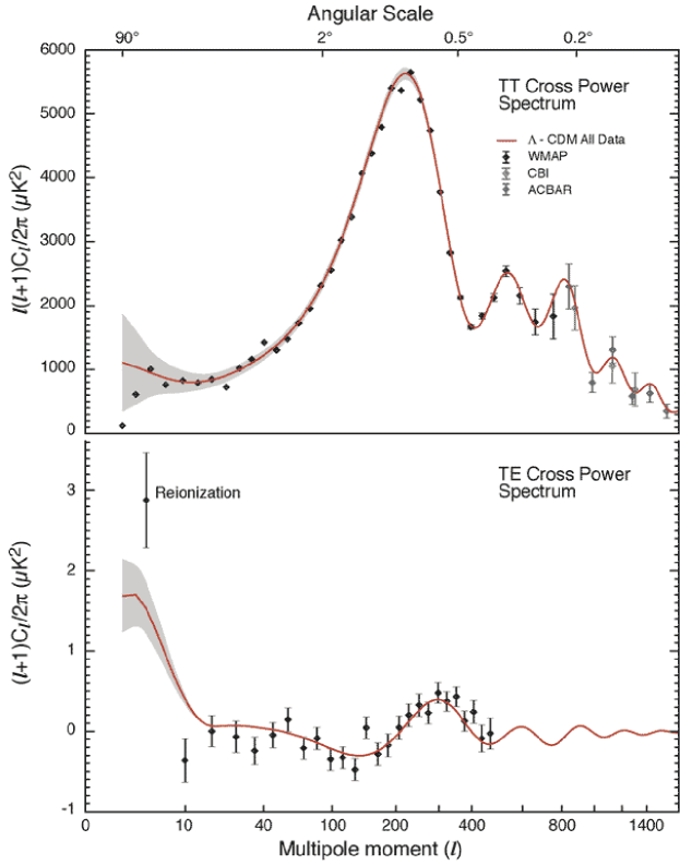
Particularly exciting is that WMAP did not just measure the anisotropy in the temperature of the CMB, but also its polarization. The WMAP polarization measurement provides us with what is probably the least ambiguous signal for inflationary physics: a measured anticorrelation between the polarization and the temperature fluctuations on an angular scale around $\ell=100$, evident in the bottom panel of Fig. 1. This feature is important because it is an essentially foreground-free measurement of correlations in primordial fluctuations on scales larger than the horizon size, a “smoking gun” for the acausal physics characteristic of inflation zaldarriaga97 . (Large-angle correlations in the temperature do not provide a clean signal of such acausal physics because of the possibility of foregrounds such as the integrated Sachs-Wolfe effect.)

Future CMB observations will improve considerably on existing data sets, especially in the measurement of the polarization signal. CMB polarization spectra divide into two types depending on their parity under reflections of the celestial sphere: even-parity, or “E-modes”, and odd-parity, or “B-modes”. The E-mode was first detected by DASI DASIemode , and the temperature / E-mode cross correlation was measured by WMAP. The B-mode signal is much smaller, and has yet to be detected. The B-mode is of particular interest for learning about inflation, because it is the only CMB signal that receives no contribution from primordial density fluctuations. Instead, the B-mode is generated entirely by primordial gravitational wave fluctuations. Since both scalar (density) and tensor (gravitational wave) fluctuations are generated during inflation, detection of tensor modes would greatly increase our ability to place constraints on the inflationary model space. In particular, the amplitude of the tensor fluctuations (unlike scalars) depends only on the value of the Hubble constant during inflation, or equivalently the potential of the scalar field driving inflation (the inflaton):

$$P_{\rm T}=\left({H\over 2\pi m_{\rm Pl}}\right)^{2}={2V\left(\phi\right)\over 3\pi m_{\rm Pl}^{4}}.$$ (1)

Therefore, if we measure the amplitude of primordial tensor fluctuations, we can determine the energy scale of inflation. This makes the B-mode polarization an important observational target for cosmology. The big question is then, how large a B-mode do we expect to be generated by a typical inflation model?

II Effective field theory and the energy scale of inflation

The prevailing prejudice in model building is that the inflaton is a fundamental field: a scalar degree of freedom in some low-energy limit of an underlying, fundamental theory such as supergravity or string theory. Therefore we expect the techniques of effective field theory, for which heavy degrees of freedom are integrated out, to be a correct description of the physics of inflation. In other words, expect the effective potential for the inflaton to be an expansion in nonrenormalizable operators suppressed by some higher energy scale, which we take to be the Planck mass:

$$V\left(\phi\right)=V_{0}+{1\over 2}m^{2}\phi^{2}+\phi^{4}\sum_{p=0}^{\infty}{\lambda_{p}\left(\phi\over m_{\rm Pl}\right)^{p}}.$$ (2)

The effective Lagrangian for the inflaton will also in general contain corrections (also suppressed by the Planck mass) to kinetic terms, but we need not consider these for the purpose of the current argument. The important feature of this construction is that the effective theory is only self-consistent for $\phi<<m_{\rm Pl}$, otherwise the series expansion for the effective potential (2) will not in general be convergent. The question we wish to answer here is: how well does such a construction work in the context of inflation?

To illustrate, we consider the simple case of a monomial “small field” potential with height characterized by a scale $\Lambda$ and width characterized by a scale $\mu$,

$$V\left(\phi\right)=\Lambda^{4}\left[1-\left({\phi\over\mu}\right)^{p}\right].$$ (3)

For potentials of this form, inflation takes place when the field value is small, $\phi\ll\mu$, and the slope of the potential is also small, $V^{\prime}\ll V$ so that the field is slowly rolling and the contribution of the potential to the energy density of the field dominates over the contribution of the kinetic energy. Eq. (3) represents the form of the potential near its maximum $\phi=0$. Inflation ends and reheating takes place when the field value is comparable to the width parameter $\phi\sim\mu$. So the field travels a distance $\Delta\phi\sim\mu$ during inflation. Therefore our assumption of a valid effective field theory expansion (2) is only consistent if $\Delta\phi\sim\mu\ll m_{\rm Pl}$ lyth96 . We first take the case $p=2$. The spectral index of scalar fluctuations can be calculated to be

$$n=1-{1\over 4\pi}\left({m_{\rm Pl}\over\mu}\right)^{2}.$$ (4)

We see that the scale-invariant limit is reached for $\Delta\phi\sim\mu>>m_{\rm Pl}$. For $n>0.95$, we must have $\mu>1.3m_{\rm Pl}$, and we expect effective field theory to break down at some point during the inflationary evolution. Such potentials predict a tensor/scalar ratio $r\equiv(C^{T}_{2}/C^{S}_{2})\simeq 0.01$ for $n\simeq 0.95$. This is not the most extreme example. For a potential of the form $V\left(\phi\right)=\lambda\phi^{4}$, which predicts a large tensor/scalar ratio $r\sim 0.1$, the field travels $\Delta\phi\sim 4m_{\rm Pl}$ during inflation. However, consider a potential of the form (3) with $p=4$. The spectral index of scalar fluctuations is given by $n\simeq 0.95$ regardless of the values of the fundamental scales $\Lambda$ and $\mu$ in the potential kinney95 . So, unlike the case of the quadratic potential, it is perfectly consistent with observation to have a potential with $\Delta\phi\sim\mu\ll m_{\rm Pl}$. However, one does this at the price of having a vanishingly small tensor/scalar ratio, $r\ll 10^{-3}$.

Lyth lyth96 showed this to be true in general. Subject to the condition of a nearly scale-invariant spectrum, the height of the potential can be written in terms of the tensor/scalar ratio $r$ as approximately

$$\Lambda\sim\left({r\over 0.7}\right)^{1/4}\times 1.8\times 10^{16}~{}{\rm GeV}.$$ (5)

This is the familiar result that a significant contribution of tensor fluctuations to the CMB requires that inflation take place at a high energy scale. More important for the discussion here is that the width of the potential can also be related to the tensor/scalar ratio

$${\Delta\phi\over m_{\rm Pl}}\sim 0.5\left({r\over 0.07}\right)^{1/2}.$$ (6)

This means that for a tensor/scalar ratio of order $0.1$, the field must travel a distance $\Delta\phi>m_{\rm Pl}$ during inflation, so that the effective field theory expansion (2) must break down at some point during inflation. An effective potential that works near the beginning of inflation will be divergent near the end of inflation, and the entire description in terms of an effective Lagrangian is invalid. This fact has been used as an argument, based on self-consistency, for expecting a very small tensor/scalar ratio in a realistic inflationary universe.

This is a discouraging conclusion, because it means that the signature of primordial gravitational waves, in particular the B-mode component of the CMB, will be unobservably small. Knox and Song knox02 have shown that foregrounds from gravitational lensing by cosmological structure place a fundamental lower limit on how well the B-mode can be measured, corresponding to a lower limit on the tensor/scalar ratio of about

$$r>6\times 10^{-4},$$ (7)

which corresponds to an energy scale for inflation of roughly

$$\Lambda>3.2\times 10^{15}\ {\rm GeV}.$$ (8)

If the energy scale of inflation is below this limit, the B-mode (and hence the primordial gravitational wave background) will be unobservable in the CMB. (A recent paper hirata03 indicates that it may be possible to use a more optimal estimator to improve the Knox and Song limit by as much as a factor of two. This does not substantially alter the discussion here.)

III The flow approach to inflationary evolution

Arguments based on effective field theory, however, are not the only way to look at the dynamics of inflation. The inflaton, for example, may not be a fundamental field – all that is necessary for the predictions of single “field” inflation to be valid is that the evolution of the spacetime be governed by a single order parameter. It is desirable to look at the predictions of inflation without resorting to assumptions about effective field theory. One way to do this is to reformulate the dynamical equations for inflation as flow in the space of dimensionless slow roll parameters flowpapers . A major advantage of this approach is that it removes the field from the dynamical picture altogether, so that we can study the generic behavior of slow roll inflation without making assumptions about the nature of the underlying particle physics. To construct the hierarchy of flow equations, we start with the slow roll parameters

$$\epsilon\equiv{m_{\rm Pl}^{2}\over 4\pi}\left({H^{\prime}\left(\phi\right)\over H\left(\phi\right)}\right)^{2},$$ (9)

and

$$\eta\equiv{m_{\rm Pl}^{2}\over 4\pi}\left({H^{\prime\prime}\left(\phi\right)\over H\left(\phi\right)}\right).$$ (10)

To lowest order, the observables $r$ and $n$ are given to lowest order in slow roll by

$$r \simeq 10\epsilon,$$ (11)

$$n-1 = 4\epsilon-2\eta\equiv\sigma.$$ (12)

Here we have introduced $\sigma\equiv 4\epsilon-2\eta$ for notational convenience. These can be seen as the first members of an infinite hierarchy of slow roll parameters liddle94

$${}^{\ell}\lambda_{\rm H}\equiv\left({m_{\rm Pl}^{2}\over 4\pi}\right)^{\ell}{\left(H^{\prime}\right)^{\ell-1}\over H^{\ell}}{d^{(\ell+1)}H\over d\phi^{(\ell+1)}}.$$ (13)

Each of these parameters can be written as a function of the number of e-folds $N$ before the end of inflation, where

$${d\over dN}={m_{\rm Pl}\over 2\sqrt{\pi}}\sqrt{\epsilon}{d\over d\phi},$$ (14)

and we have an infinite series of differential flow equations describing the inflationary evolution

$${d\epsilon\over dN} = \epsilon\left(\sigma+2\epsilon\right),$$ (15)

$${d\sigma\over dN} = -5\epsilon\sigma-12\epsilon^{2}+2\left({}^{2}\lambda_{\rm H}\right),$$ (16)

$${d\left({}^{\ell}\lambda_{\rm H}\right)\over dN} = \left[{1\over 2}\left(\ell-1\right)\sigma+\left(\ell-2\right)\epsilon\right]\left({}^{\ell}\lambda_{\rm H}\right)+{}^{\ell+1}\lambda_{\rm H}.$$ (17)

The field has disappeared from the equations of motion altogether, although the underlying assumption of dynamics controlled by a single order parameter is of course still present. The flow equations allow us to investigate the model space for inflation using Monte Carlo techniques. Since the dynamics are governed by a set of first-order differential equations, the cosmological evolution is entirely specified by choosing values for the slow roll parameters $\epsilon,\sigma,{}^{2}\lambda_{\rm H},\ldots$. Choosing such a point in the parameter space completely specifies the inflationary model, including the scalar field potential, which can be reconstructed for each choice, so-called “Monte Carlo reconstruction” montecarlorecon . The observable predictions for a given model can be evaluated as follows:

• Pick a point in the parameter space $\epsilon,\sigma,{}^{2}\lambda_{\rm H},\ldots$

• Evolve forward in time until inflation ends, or reaches a late-time attractor.

• From the end of inflation, evolve backward in time about 60 e-folds, and calculate the values of the slow roll parameters at that point.

• Calculate the observables $r$, $n$, $dn/d\ln{k}$.

This procedure can be performed numerically for a large number of randomly chosen initial conditions. Instead of specifying a potential and calculating the predictions for that model (“hand crafting” inflation), we can process models on an industrial scale, investigating the behavior of millions of possibilities for the inflationary dynamics. The result is very interesting: models do not uniformly cover the observable parameter space, but instead cluster around attractor regions. How well do the attractors correspond to the expectations from effective field theory? Not especially closely. Figure 2 shows the models plotted in the $r,n$ plane, showing that there is a significant concentration of models with nonzero tensor/scalar ratio $r$.

Figure 2: Models generated by Monte Carlo plotted in the $(n,r)$ plane. The solid line is the power-law inflation fixed point $n=1-2r/(10-r)$.

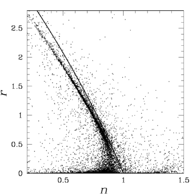
Figure 3 shows the same points plotted logarithmically in tensor/scalar ratio, with the lower bound from Knox and Song marked on the plot. There is a substantial population of dynamically valid inflation models with a tensor scalar ratio that is in principle observable, and there is no compelling reason to rule such models out. Observation of a significant tensor/scalar ratio would be a strong indication of some kind of exotic physics driving inflation, which is not adequately captured by a description in terms of a low-energy effective field theory with operators suppressed by powers of the Planck scale. Such a result would be of great interest from the standpoint of inflationary model building, but would not in itself weaken inflation as a viable theory.

Figure 3: n vs log r. The horizontal line is the lensing limit of Knox and Song. There is a substantial population of models with a large enough tensor/scalar ratio to be detectable above the lensing foreground.

IV The current observational situation and future prospects

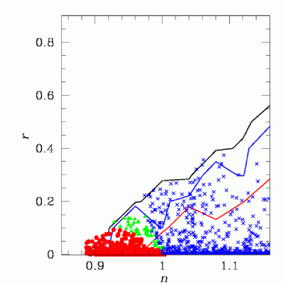
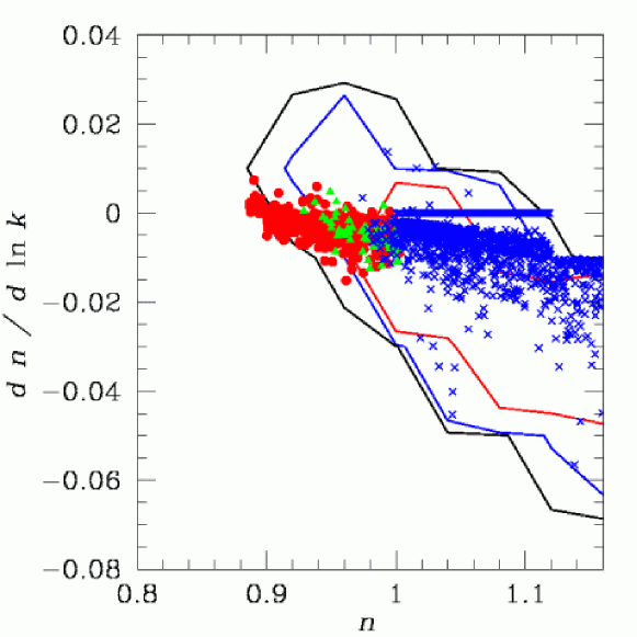
What are the prospects in the near future for detection of a tensor contribution to the CMB? Certainly, it is not likely that we will be able to approach the lensing bound on the B-mode any time soon. Current limits on the size of the tensor contribution to the CMB are still quite crude, although the recent WMAP result represents a substantial step forward. Figure 4 kkmr shows the constraint on the $n,r$ plane from the WMAP data set in conjunction with seven additional CMB data sets (BOOMERanG-98 ruhl , MAXIMA-1 lee , DASI halverson , CBI cbi , ACBAR acbar , VSAE grainge , and Archeops benoit ). Figure 5 kkmr shows the constraint in the $n,dn/d\log{k}$ plane, showing a preference for a negative running of the spectral index with scale, consistent with the results of the data analysis done by the WMAP teampeirisetal . The points plotted are models generated by Monte Carlo evaluation of the flow equations consistent with the data to $3\sigma$, and are coded by their “zoology”: small field, large field, and hybrid. We see that while no class of models is ruled out by the data, the hybrid class shows the greatest consistency with the best-fit region. There is in fact a population of hybrid models with a strong negative running of the spectral index, showing that the WMAP best fit is quite consistent with what one might expect from inflation. Deviations from the limiting case of a scale-invariant power-law spectrum are exactly what one ought to expect in a realistic inflationary cosmology: astrophysical observations probe the last sixty e-folds, i.e. the end of inflation, when the limiting behaviors of slow roll are beginning to break down. In terms of the current data, inflation is in excellent shape as a model for production of the primordial density fluctuations.

Figure 4: Errors from current CMB data on the $(r,n)$ plane. The contours represent $1\sigma$, $2\sigma$, and $3\sigma$ errors. The points are models generated by Monte Carlo, categorized into small-field (red, circles), large-field (green, triangles), and hybrid (blue, crosses). No class of models is yet ruled out by the data.

Figure 5: Errors from current CMB data on the $(n,dn/d\log{k})$ plane. Contours represent $1\sigma$, $2\sigma$, and $3\sigma$ errors, with the models plotted as in Fig. 4. Note that the region with negative running is well populated by models, especially of the hybrid class, indicating that the WMAP best fit is easily accomodated by simple inflationary models.

What does WMAP tell us about the energy scale of inflation? As one would expect from the broad range of tensor/scalar ratios consistent with the data, the height of the potential during inflation is poorly determined. Figure 6 kkmr shows an ensemble of potentials consistent with the current CMB data, generated by Monte Carlo reconstruction montecarlorecon .

Figure 6: Potentials consistent with current CMB limits generated by Monte Carlo reconstruction (color codes are the same as in Figs. 4 and 5). The horizontal line indicates the lensing limit of Knox and Song. The energy scale of inflation is not well constrained by current observations, and could in fact be many orders of magnitude below what is in principle detectable.

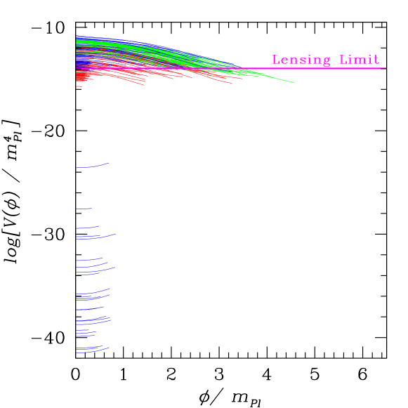
From Fig. 6 we see that a wide range of energy scales are consistent with existing data, including scales large enough to generate an (in principle) observable tensor contribution to the CMB anisotropy. We can also see in concrete form that the width of such potentials is large enough in Planck units to signal a breakdown of the effective field theory approximation (2).

While a tensor/scalar ratio $r>6\times 10^{-4}$ is observable in principle, it is very useful to understand what is going to be possible in practice in the near future. Figure 7 shows the expected errors from three experiments, plotted against models on the $n$ vs. $\log{r}$ plane: (1) a cosmic-variance limited (i.e. ideal) temperature-only CMB map, (2) the Planck Surveyor satellite, including measurement of CMB polarization Planck , and (3) a hypothetical measurement with the same angular resolution as Planck, but with a factor of three increase in sensitivity kinney98 . While the lensing limit on the B-mode is well below the expected sensitivity of these measurements, a tensor/scalar ratio of $r\sim 0.01$ is well within reach of presently feasible observations. It may well be possible to do considerably better.

Figure 7: Inflation models plotted with error bars from expected and hypothetical measurements. The dots are models generated by Monte Carlo. The solid areas are the predictions of specific potentials: $V\propto 1-(\phi/\mu)^{p}$ (green, lower area), $V\propto 1-(\phi/\mu)^{2}$ (red, central area), $V\propto\phi$ (black, third line from top), $V\propto\phi^{p}$ (cyan, second line from top), and $V\propto\exp(\phi/\mu)$, (blue, top line). The error bars are for (a) a cosmic-variance limited temperature-only measurement, (red, outside contour), (b) the Planck Surveyor satellite including polarization (blue, middle contour), and (c) a hypothetical measurement with the same angular resolution as Planck but a factor of three higher sensitivity (black, inner contour). The horizontal line shows the lensing limit of Knox and Song.

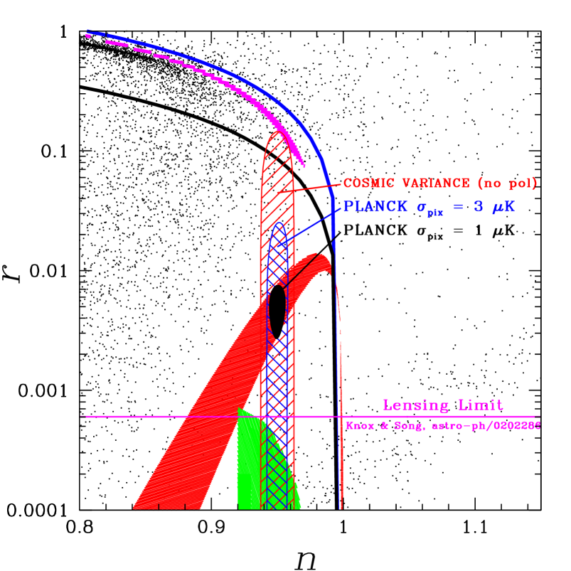
This level of sensitivity represents an important observational milestone. A detection of tensor modes in the CMB with $r>0.01$ will be an indication that the effective field theory expansion (2) is not self-consistent, and that therefore inflation in the early universe is begin driven by some sort of exotic physics, for example the holographic renormalization group flow proposed by Larsen et al. rginfl . A non-detection, however, would validate low-energy effective field theory as a viable tool for inflationary model building, which would leave the door open for more conventional descriptions of the inflaton, such as inflation from supersymmetric moduli fields, pseudo-Nambu Goldstone modes, or other conventional particle physics candidates. (See Ref. lythriotto for a review.)

V Conclusions

Recent CMB observations, especially the results from the WMAP satellite, represent a sea change in our understanding of the physics of the early universe. For the first time, it is possible to place meaningful constraints on theories of the of the universe at its earliest stages, in particular the inflationary paradigm. If inflation really is the correct model for the evolution of the early universe and for the generation of primordial perturbations, a central question is: what was the energy scale of inflation? Determining the answer to this question requires a measurement of the primordial gravitational wave (tensor) fluctuations generated during inflation. The curl, or “B-mode” component of CMB polarization is a particularly sensitive probe of primordial tensor modes, because the B-mode does not receive contributions from primordial density fluctuations. However, gravitational lensing by cosmological structure also generates B-mode polarization, and this foreground cannot be perfectly subtracted. This places a lower limit on sensitivity to a primordial B-mode and hence on the amplitude of gravitational wave fluctuations. This can be expressed in terms of a lower limit on the tensor/scalar ratio $r>6\times 10^{-4}$ knox02 .

Expectations based on the self-consistency of a low-energy effective field theory description of inflation, however, argue for a very small tensor/scalar ratio and a corespondingly low energy scale for inflation lyth96 . If this theoretical prejudice is correct, the primordial B-mode will almost certainly be too small to be detected. Nonetheless, looking at inflationary model building from the somewhat broader perspective of the flow formalism shows that there is a substantial population of dynamically viable inflation models with an observably large tensor/scalar ratio. The expected sensitivity of forthcoming CMB observations such as the Planck surveyor or (perhaps) dedicated searches for the B-mode polarization can realistically reach a sensitivity of $r\sim 0.01$, which is sufficient to distinguish between conventional effective field theory descriptions of inflation and models based on some more exotic order parameter. Whether the search for primordial B-mode polarization in the CMB is ultimately a success or a failure, we will learn something important about the physics of inflation.