Stellar density distribution in the NIR on the Galactic plane at longitudes 15-27 deg.
Clues for the Galactic bar ?

Garzón et al. (1997), López-Corredoira et al. (1999) and Hammersley et al. (2000) have identified in TMGS and DENIS data a large excess of stars at l=27^∘ and b=0^∘ which might correspond to an in-plane bar. We compared near infrared CAIN star counts and simulations from the Besançon Model of Galaxy on 15 fields between 15^∘ and 45^∘ in longitude and -2^∘ and 2^∘ in latitude. Comparisons confirm the existence of an overdensity at longitudes lower than 27^∘ which is inhomogeneous and decreases very steeply off the Galactic plane. The observed excess in the star distribution over the predicted density is even higher than 100%. Its distance from the sun is estimated to be lower than 6 kpc. If this overdensity corresponds to the stellar population of the bar, we estimate its half-length to 3.9$\pm$0.4 kpc and its angle from the Sun-center direction to 45$\pm$9 degrees.

1 Introduction

Star counts have been used for years to examine at various levels of detail the stellar contents in the Galaxy (see Paul 1993), whose structural parameters of the various morphological components are still far from being completely known. In the last two decades there has been a combined effort in this direction with the use of detailed models of stellar galactic distribution (Bahcall & Soneira 1980; Robin & Crézé 1986; Wainscoat et al. 1992; López–Corredoira et al. 2002) along with large area, high sensitivity and multicolour star count surveys. The near infrared (NIR) members of these surveys (Eaton et al. 1984, Garzón et al. 1993, Hammersley et al. 1994, López–Corredoira et al. 2000, Epchtein 1997, Skrutskie et al. 1997) are notably useful for the analysis of the galactic structure because of less interstellar extinction compared to the optical bands, in particular in the hidden on-plane areas of the inner Galaxy. It is in these zones that the morphological structures are less well studied.

The effect of the high extinction towards the inner Galaxy along the Galactic plane, added to the position of the Sun very near to the plane itself (Hammersley et al. 1995), makes it particularly difficult to detect large scale stellar structures in the central part of the Galaxy. There is an increasing consensus that the Galaxy is of barred type (see Garzón 1999 for a review), but there is still a considerable controversy about the morphology and stellar content of the bar.

Hammersley et al. (2000) has recently derived arguments for the Galactic bar to be of half-length of roughly 4 kpc and with a position angle with the sun-center direction of around $43\deg$, by observing from new NIR star count data an excess of stars at longitudes on the Galactic plane at l$\leq$27^∘ and assuming them to belong to the bar population. To continue this research work (see also López–Corredoira et al. 2001) in the field of the structure of the inner Galaxy we have made use in this paper of the large NIR star count database obtained with the CAIN camera at the Teide Observatory (Hammersley et al. 2000) together with the Besançon model of the Galaxy (Robin & Crézé 1986; Bienaymé et al. 1987; Robin et al. 2003) to examine the excesses in both the magnitude and the colour histograms of the data with respect to the model predictions. This study permits us on the one hand to confirm with an independent method the existence of this extra density, and allows us on the other hand to derive considerations about its structure. Indeed, since the Besançon model does not contain any galactic component other than the thin disc (and possibly the triaxial bulge at the innermost field) in the regions of interest, as will be described in the next sections, any excess observed in the stellar density compared to the model prediction may then be used to analyze the morphological extent of such an extra population.

This paper is organized as follows. We briefly describe the star count data and the Besançon model used in this work. We then discuss the method of deriving the extinction distribution along the line of sight from the data alone, which is then used in the model for the predictions.Those predictions are then compared with the data in two different planes: magnitude and colour counts, which both serve for the analysis. We provide conclusions describing the model itself and the derived geometry for the component responsible for the excesses.

2 The Besançon Model of the Galaxy

The approach of the Besançon model is slightly different from the ones used previously to study the bar. Here,we give a brief description of the model, dealing particularly with the thin disc population model. More details can be found in Robin & Crézé (1986), Bienaymé et al. (1987) and Robin et al. (2003).

2.1 Global description

The Besançon Model of Stellar Population Synthesis, developed in the visible, near and mid infrared, aims at giving a global 3-dimensional description of the Milky Way, including stellar populations such as the thin disc, outer bulge, thick disc and spheroid, as well as dark halo and interstellar matter.

Its approach is semi-empirical: both theoretical schemes (stellar evolution, galactic evolution, galactic dynamics) and empirical laws found in the literature are used. Boltzmann and Poisson equations are used to make the model dynamically self-consistent in the direction perpendicular to the plane. Artificial catalogues of stars are produced, giving both the fundamental characteristics of stars (age, distance, absolute magnitudes, kinematics) and observable ones (apparent magnitudes, colours, proper motion, radial velocities) directly comparable with observations. Absorption, photometric errors and Poisson noise are also added to make simulations as close as possible to observations.

The Besançon model has been used to constrain the density law or the luminosity function of the stellar populations: thin disc (Ruphy et al. 1996; Haywood et al. 1997), thick disc (Robin et al. 1996; Reylé & Robin 2001), spheroid (Robin et al. 2000) and bulge (Picaud & Robin, in preparation).

2.2 Thin disc

In the studied region, thick disc and spheroid populations give a negligible contribution, and those from the bulge likely only contaminate star counts at the innermost field (l=15^∘). Thus, the only dominant stellar population taken into account by the model is the thin disc. Its density is modeled as the Einasto law (1979): the thin disc is divided in 7 age components and each component distribution is described by an axisymmetric ellipsoid. The first component (0-0.15 Gyr) is called the young disc and the 6 other ones form the old disc, which only is presented here because of the very small number of stars belonging to the young one. The density law of each ellipsoid of the old disc is the subtraction of two modified exponentials, the second one representing the central hole:

$$\rho=\rho_{0}\times[\exp(-\sqrt{0.25+(\frac{a}{R_{d}})^{2}})-\exp(-\sqrt{0.25+(\frac{a}{R_{h}})^{2}})]$$

with $a^{2}=R^{2}+\left(\frac{Z}{\epsilon}\right)^{2}$, where:

• $R$ and $Z$ are the cylindric coordinates

• $\epsilon$ is the axis ratio of the ellipsoid which increases with the age of the component. The 6 axis ratios of the old thin disc are presented in Table LABEL:axisratios.

• $R_{d}$ is the global scale length of the disc and $R_{h}$ is the global scale length of the hole. In the present version of the Besançon model, we use $R_{d}$=2.37 kpc and $R_{h}$=1.31 kpc, deduced from model fitting toward the inner Galaxy (Picaud & Robin, in preparation).

• The normalization $\rho_{0}$ was deduced from the local luminosity function (Jaheiss et al, private communication).

age (Gyr)	$\epsilon$
0.15-1	0.0268
1-2	0.0375
2-3	0.0551
3-5	0.0696
5-7	0.0785
7-10	0.0791

Table 1: Axis ratios of the 6 age components of the old thin disc.

The distributions in $M_{v}$, $\log{T_{eff}}$, $\log{g}$ are deduced from an evolution model described in Haywood et al. (1997). Absolute magnitudes in K are computed from the corresponding V absolute magnitudes using the semi-empirical model of atmospheres from Lejeune et al. (1997, 1998). Disc density parameters and further changes in the luminosity function are explained in Robin et al. (2003).

2.3 Extinction

The Besançon model includes its own extinction model which follows the young thin disc distribution, with a scale length of 4 kpc, an equivalent scale height of 140 pc, and a normalization which can be modulated. However, this model can be replaced by another distribution as needed.

For this study, we have preferred to model the extinction without using the Besançon simulations to avoid a possible bias in the comparisons of the model with the data. The determination of the extinction distribution in each field will be described in section 4.

3 Observations

Since 1999 the IAC group has been building a Galactic survey by using CAIN, the NIR camera on the 1.5-m Telescopio Carlos Sánchez (TCS) (Observatorio del Teide, Tenerife). Observations of a series of 20 x 12 arcmin² (i.e., a total area of approximately 0.07 deg²) have been made along the Galactic plane between $l=0^{\circ}$ and $l=220^{\circ}$, together with some off-plane series (mainly in b=$\pm 2^{\circ},\pm 5^{\circ}$ and $\pm 10^{\circ}$). The survey uses the J (1.25$\mu$m), H (1.65$\mu$m), and K_short (2.17$\mu$m) standard bands, with limiting magnitudes of 17, 16.5 and 15.2 respectively. This provides almost one magnitude deeper coverage than 2MASS or DENIS surveys in the K-band (Struskie et al. 1997; Epchtein et al. 1997), which is very useful for the study of the inner galactic regions such as those considered in this paper. For the fields we used here, the seeing was typically of 1 arcsec, and data were obtained only in photometric conditions. The main characteristics of the 15 chosen fields and photometric bands used are summarized in Table LABEL:tabcamps.

l (deg)	b (deg)	area (x 10-2 deg${}^{2})$	completeness limits (band used)
15	0	6.95	16.8 ($J$)	14.8 ($K_{s}$)
20	0	6.97	16.8 ($J$)	14.8 ($K_{s}$)
21	0	6.99	16.8 ($J$)	14.8 ($K_{s}$)
26	0	12	16.8 ($J$)	14.6 ($K_{s}$)
26	2	6.95	16.4 ($J$)	14.8 ($K_{s}$)
27	0	6.97	16.4 ($J$)	14.4 ($K_{s}$)
27	0.5	6.97	16.4 ($J$)	14.8 ($K_{s}$)
27	-0.5	6.96	16.4 ($J$)	14.8 ($K_{s}$)
27	1	6.91	17 ($J$)	15 ($K_{s}$)
28	0	6.93	17 ($J$)	15 ($K_{s}$)
32	0	6.92	17 ($J$)	15 ($K_{s}$)
33	-2	7.03	16.4 ($J$)	14.8 ($K_{s}$)
37	2	7.03	16.8 ($J$)	15.4 ($H$)
40	0	7.05	16.8 ($J$)	14.8 ($K_{s}$)
45	0	6.99	16.6 ($J$)	14.6 ($K_{s}$)

Table 2: CAIN survey selected regions used in this paper.

4 Extinction from K-giants

Extinction changes very much from one field to another in and close to the Galactic plane, and a good determination of its distribution is needed to compare data and simulations in this region. This is why a global extinction model is not sufficient and the distribution of extinction along the line of sight must be determined field by field.

4.1 Method of extraction of the extinction distribution

López-Corredoira et al. (2002) (hereafter L02) developed a method to obtain the star density and interstellar extinction along a line of sight by extracting a well-known population (spectral type K2III) from the infrared colour-magnitude diagrams (hereafter CMD). The method is extensively described in L02, so we give only a brief summary here.

($J-K,m_{K}$) CMDs are built for each field. In the diagrams, stars of the same spectral type (which would mean that they have about the same absolute magnitude but are located at different distances from the Sun) will be placed at different locations in the CMD. The effect of distance alone shifts the stars vertically, while extinction by itself shifts the stars both horizontally and vertically. Combinations of these effects, plus some intrinsic dispersion in absolute magnitude and/or spectral type, cause the red clump giant stars, which constitute the majority of the disc giants (Cohen et al. 2000; Hammersley et al. 2000), to form a diagonal broad branch running from top left to bottom right on the CMDs.

In order to isolate the red clump sources, count histograms have been made by making horizontal cuts (i.e. running colour) through the CMDs at fixed $m_{K}$. A Gaussian function was then fitted to the histogram to determine the position of the peak in each cut.

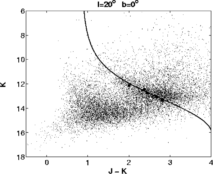
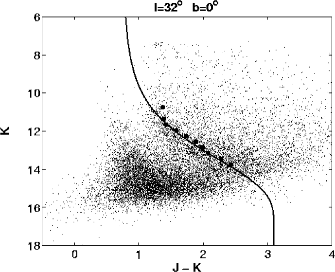
Figure 1: CMDs for two of the fields studied here. Maxima obtained by a Gaussian fitting to star distribution in the red clump strip are over-plotted. The solid line shows the fitted trace assigned to the red clump population affected by varying extinction along the line of sight.

The extinction A${}_{K}(m_{K})$, to a distance $r$, can be determined by tracing how the (J-K) of the peak of the red clump counts changes with $m_{K}$. The extinction is calculated for any given $m_{K}$ using the measured $(J-K)$ of the peak, the intrinsic mean colour excess definition, and the interstellar extinction values for $\frac{A_{J}}{A_{V}}$ and $\frac{A_{K}}{A_{V}}$ given by Mathis (1990).

$$A_{K}=\frac{(J-K)-(J-K)_{0}}{1.61}$$ (1)

Finally, the extinction law ($A_{K}$ vs. $r$) can be built for each field by using a suitable transformation for the distance along the line of sight:

$$r=10^{\frac{m_{K}-M_{K}+5-A_{K}(r)}{5}}$$ (2)

Uncertainties in the method, such the metallicity effects for the clump giants, the effect of the dwarf contamination in the K-giant strip, or differences between the real red clump distribution and the Gaussian function are fully described in L02.

4.2 Absolute magnitude calibration

The method described above can provide spatial information from the CMDs, and the only assumption being made is that the absolute magnitudes of all the sources being extracted is more or less fixed. In order to deduce the distribution of extinction along the line of sight, absolute magnitudes and colors of stars must be assigned. In L02, the peaks were identified as pertaining to the K2III stars since they are by far the most prominent population, according to the updated ”SKY” model (Wainscoat et al. 1992; M. Cohen, private communication)(see Fig.2 in L02 for details). The K2III population mean absolute magnitude and the intrinsic color were assumed to be $M_{K}=-1.65$ and $(J-K)_{0}$=0.75, with a gaussian dispersion of 0.3 mag in absolute magnitude and 0.2 in colour. However, in the present study, the absolute magnitude and intrinsic color values must be the ones used in the Besançon model to get a consistent analysis of the data. The Besançon model predicts a very prominent population of K1 giants with an absolute magnitude of $M_{K}$=-1.85 and an intrinsic colour $(J-K)_{0}$=0.64 (Fig.2). These values are slightly different from those considered initially in L02. The determination of spectral types in the model is taken from De Jager & Nieuwenhuijzen (1987).

Figure 2: Distribution of K absolute magnitudes and $(J-K)_{0}$ colours according to the Besançon model. The K0 counts are represented with dotted lines, the K1 with dotted-dashed lines and the K2 with dashed lines, while the continuous line represents the sum of the three counts. The maxima of the K1 plots correspond to the red clump, with an absolute magnitude of -1.85 and an intrinsic colour of 0.64.

Differences in using either the values used by L02 or those of Besançon are quantified and shown in Fig. 3. They cannot be a critical issue in the method, since the extraction of the peaks for the star distribution in the K-giant strip is independent of the subsequent analysis of the spectral type corresponding to those peaks. The change in the absolute magnitude and intrinsic colour of the population affects only the values extracted for A_K and $r$. The differences are less than 7% in extinction and less than 9% in distance (see Fig.3). Those errors are also of the same order of magnitude, or even less, than the intrinsic uncertainties of the real values for the absolute magnitude and intrinsic colour of the red clump population.

Figure 3: Extinction along the line of sight ($A_{V}$ vs $r$) obtained for the fields l=20^∘, b=0^∘(left) and l=32^∘,b=0^∘(right). The extinctions obtained assuming $M_{K}$=-1.65 and $(J-K)_{0}$=0.75 (L02) are shown with triangles while values with $M_{K}$=-1.85 and $(J-K)_{0}$=0.64 (Besançon model) are shown with diamonds. Differences are negligible, and they are only noticeable for off-plane regions where the extinction is lower, hence increasing the relative difference.

4.3 H band.

The analysis is made by using ($J-K,m_{K}$) CMDs for all the fields, except one (l=$37^{\circ}$,b=$-2^{\circ}$) where the K_s band was not available. A ($J-H,m_{H}$) CMD was used instead. The main difference between using the H band or the K_s band is related to the absolute magnitude and the intrinsic colour of the red clump population. Those values are not as well determined for the H filter as for the K_s, and they present a bigger dispersion than in K_s (Wainscoat et al. 1992). As explained in §4.2, we use the values defined in the Besançon model for the red clump population in this band ($M_{H}$=-1.65, $(J-H)_{0}$=0.5). The procedure of deriving the extinction is exactly the same as described before, but replacing $M_{K}$ and $(J-K)$ by $M_{H}$ and $(J-H)$. We are analyzing an off-plane field, and the extinction is low enough to produce significant differences in the extinction distribution obtained by using either the H band or the K_s band.

5 Data vs. model predictions

This study consists of comparisons of simulations from the Besançon model with CAIN data at longitudes 15^∘-30^∘ to detect and study the overdensity observed in previous studies (Hammersley et al. 2000, López–Corredoira et al. 1999). In this region, model counts are dominated by the thin disc population. This is why first comparisons between simulations and data were needed in disc fields in and out of the plane to verify that the Besançon model reproduces well the thin disc counts. Once this verification has been made, counts are compared on the one hand in the plane varying the longitude and on the other hand at different latitudes to extract information about both the horizontal extent and the vertical thickness of the detected overdensity.

Model simulations have been done assuming photometric errors close to those of the data and an extinction along the line of sight determined by the method described in section 4.

Comparisons are made in K_s magnitude and J-K_s colour for all fields except for the field at l=37^∘ b=+2^∘ where the K_s band was not available and was replaced by the H band, as explained before.

The values of limits given in Table LABEL:tabcamps show that in fields with high extinction, data are not complete in the J band for the faintest and most reddened stars. Star counts have then been produced until K_s=13.5 (H=14 at l=37^∘) and J-K_s=3 to ensure completeness. These new thresholds do not guarantee perfect completeness for all fields, but this study needed counts deep enough to observe the overdensity.

Figure 4: Percentage of dwarfs in Besançon simulations by bins of J-K_s (left) and K_s (right), for in-plane fields (up), and off-plane ones (bottom). A step between two zero lines (dashed lines) correspond to 50% of dwarfs.

In order to reduce the contamination of foreground dwarfs in star counts, only stars with J-K${}_{s}\geq$1.5 for in-plane fields and J-K${}_{s}\geq$0.75 for off-plane ones were selected. But the estimation (given by Fig. 4), using the Besançon simulations, of the dwarf contamination shows that there is still up to 20% of dwarfs at faint K_s and at low J-K_s for in-plane fields, and up to 40% at low J-K_s for off-plane ones. This contamination implies uncertainties in this work, especially for a quantitative study.

5.1 Disc fields

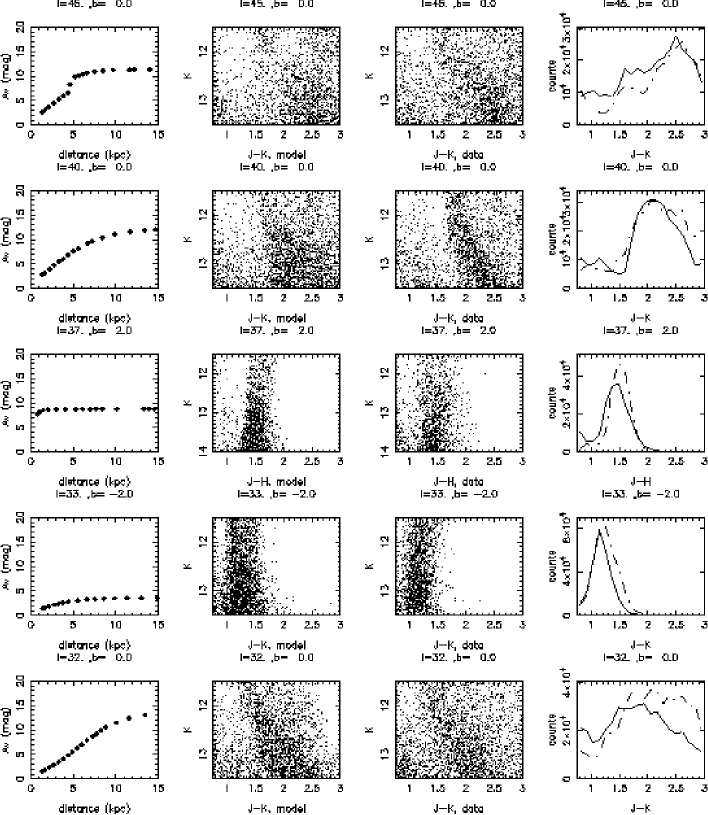
Figure 5: Extinction distributions along the line of sight, colour magnitude diagrams and colour histograms of intermediate disc fields. The CMD on the left and the dashed line at the histogram panels correspond to the Besançon simulations, while the CMD on the right and the solid line in the histograms display the CAIN data. Star counts of the colour histograms (in number of stars per magnitude bin and per square degree) are taken for 11.5 $<$ K_s $<$ 13.5

.

Model counts were compared with data on 3 fields on the galactic plane: b=0^∘ l=45^∘, 40^∘ and 32^∘, and 2 off plane fields: l=37^∘ b=+2^∘ and l=33^∘ b=-2^∘.

Extinction distributions, model and data colour-magnitude diagrams and count histograms are presented in Figure 5.

Model and data CMDs and histograms are rather close to each other, but in some fields there is a slight excess of reddest stars. The model of disc stellar evolution (Haywood et al. 1997) might overestimate the duration of late type stars and perhaps the oldest stars of these types have already become white dwarfs or planetary nebulæ. A correction has been made by rejecting giants with a spectral type later than K5 and age greater than 7 Gyr but does not eliminate all the excess. The problem of late type stars may be enhanced in off-plane fields: in these fields, stars are less reddened and most of them are below the cuts in K_s=13.5 and J-K_s=3. Moreover, because of the very small reddening, histograms of these fields may be more contaminated by foreground dwarfs even with the blue cut in J-K_s.

In any case, this excess of simulated stars is small enough to consider that the Besançon model reproduces rather well the thin disc and to continue the study on fields at l$<$30^∘.

5.2 Along the Galactic plane

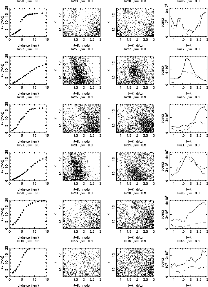
Figure 6: Colour magnitude diagrams and colour histograms of fields at l$\leq$28^∘ and b=0^∘. See caption of Figure 5 for an explanation about the content of the different panels.

In addition to the 3 on-plane disc fields (l=32^∘, l=40^∘, l=45^∘), we compared model and data on 6 fields at l$\leq$28^∘ and b=0^∘ : l=28^∘, l=27^∘, l=26^∘, l=21^∘, l=20^∘, l=15^∘. Extinction distributions, colour-magnitude diagrams and histograms are presented in Figure 6.

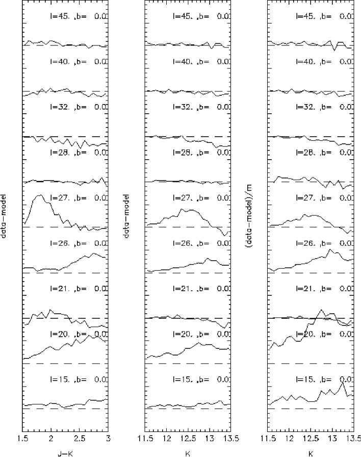
Figure 7: Difference distribution vs. magnitude along the Galactic plane. Dashed lines are zero reference lines. The left and center histograms present the absolute difference ’data minus model’ in J-K_s colour and K_s magnitude, and the range between two zero lines corresponds to 70000 mag^-1deg^-2. The right ones present the relative difference in K_s counts($m$ being the average of model counts for 11.5 $\leq$ K_s $<$ 13.5) and the step between two zero lines corresponds to 400%. Star counts are compared in 1.5 $\leq$ J-K_s $<$ 3 and 11.5 $\leq$ K_s $<$ 13.5.

Figure 7 presents the histograms of differences ’data minus model’ along the galactic plane. In order to compare the relative excess at different longitudes apart from changes in disc density from one field to another, we computed relative differences $\frac{\mbox{data-model}}{m}$ where $m$ is the average of simulated counts over the full magnitude range.

These histograms show clearly the existence of an excess of stars at l$\leq$27^∘ (except for the field at l=$21^{\circ}$), contrary to fields at l$\geq$28^∘ where data and model star counts are similar.

The observed excess is too large to be explained by a bad determination of the extinction distributions along the line of sight. Furthermore, color magnitude diagrams in the Figure 6 show that the giant clumps are rather well reproduced for most fields, and histograms in J-K_s in the same Figure have similar shapes : only the heights of the maxima change. Moreover, data are not always totally complete for K close to 13.5, especially for the most reddened stars in the fields with highest extinction, which may attenuate the data excess in these fields.

A possible contamination in the counts by stars of the Scutum Spiral arm cannot explain the observed overdensity a l$\leq$27^∘ as the impact of the arm is only expected at the position of the tangential point to the lane of stars, located at l=33^∘, with a negligible contribution for l$<$31^∘ (Hammersley et al. 1994).

Except for the discrepancies in the most reddest part of the CMDs (which corresponds to an excess of stars while the great discrepancies at low longitudes correspond to a deficit of the model), comparisons of disc fields have shown that the Besançon model reproduces rather well the galactic disc between l=32^∘ and l=45^∘. Thus, a bad modeling of disc scale length or equivalent disc scale heights cannot explain the excess of stars, and changes made by realistic modifications of them would not be sufficient to remove this excess.

But this is not the same thing for the hole scale length which, is not relevant at l$>$32^∘. Fig. 8 gives the results in 3 fields b=0^∘ and l=15^∘,20^∘,25^∘ for 3 different hole scale lengths: 0.5, 1 and 1.5 kpc. Values lower than 0.5 kpc would not significantly change the histograms, and values greater that 1.5 are not very realistic. But between these two limits, one can see that the value of the scale length has a great influence on the excess. Nevertheless, this influence decreases with longitude and cannot explain all the excess. But it implies another uncertainty for a quantitative study.

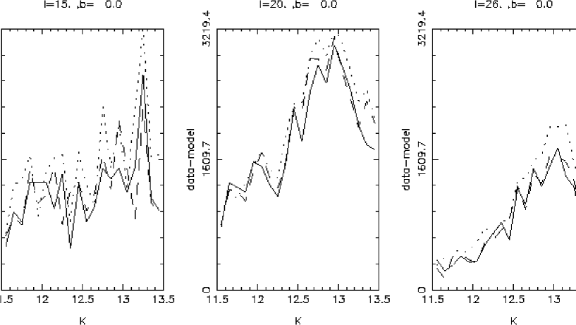
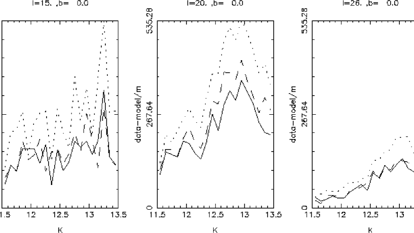
Figure 8: Absolute (upper) and relative (bottom) histograms of difference ’data minus model’ in K_s for 3 different hole scale length: 0.5 kpc (solid lines), 1 kpc (dashed lines) and 1.5 kpc (dotted lines). Units are mag^-1.deg^-2 for absolute histograms and % for relative ones.

To summarize, the analysis of the histograms of Fig. 7 confirm the existence of an overdensity with respect to the thin disc predictions. The overdensity begins at l=27^∘ and extends at least until l=15^∘, but seems to be inhomogeneous and locally disappears at l=21^∘.

5.3 Out of the Galactic plane

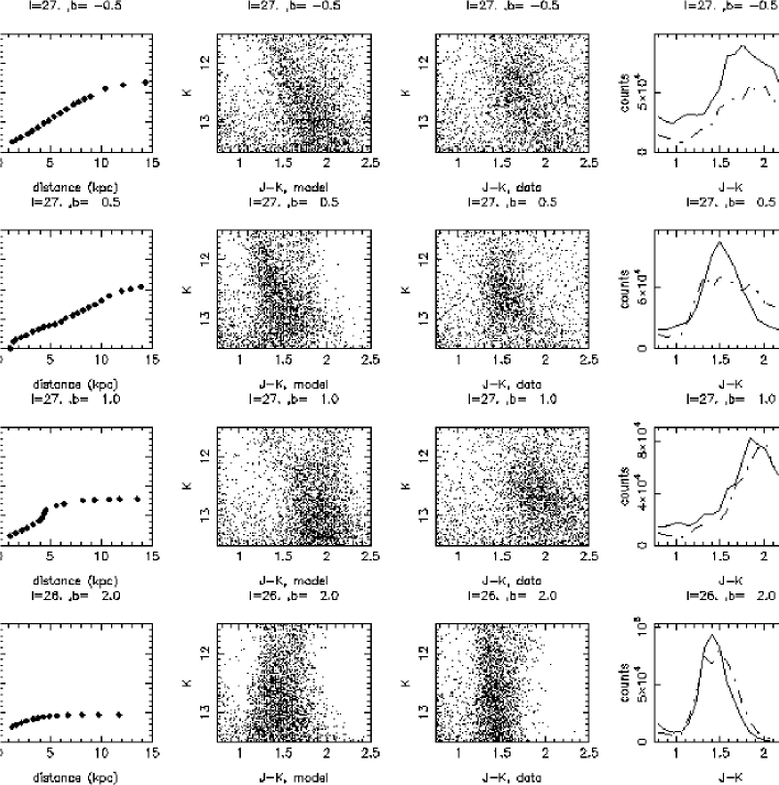
Figure 9: Extinction distributions, colour magnitude diagrams and colour histograms of fields at b$\neq$0^∘. Explanations of the graphs are given in Figure 5.

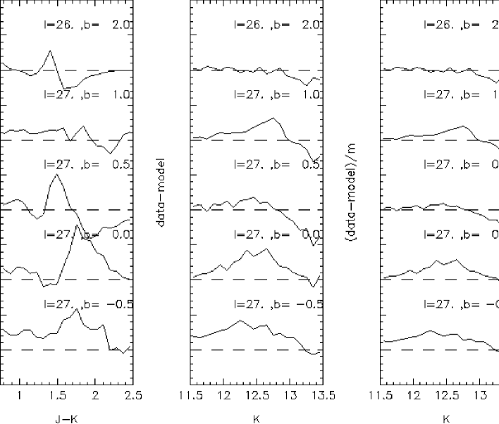
Figure 10: Histograms of differences. Explanations of the graphs are given in Figure 7 and the same scales are used. However we have changed the cuts on J-K for histograms due to the fact that the reddening is now lower than in the in-plane regions. The new colour range is 0.75 $\leq$ J-K_s $<$ 2.5.

We have studied 4 fields out of the galactic plane, roughly at longitudes coinciding with the end of the overdensity presented in the previous section : l=27^∘ b=-0.5^∘,+0.5^∘,+1^∘, and l=26^∘ b=+2^∘. The colour-magnitude diagrams and the difference histograms of theses fields are presented respectively in Figure 9 and 10.

The difficulties in modeling the extinction (even if it is low) in these fields or to select the giant clump because of the low number of stars, added to the problem of the Besançon model predictions on disc fields out of the plane make a detailed study of the overdensity difficult out of the galactic plane.

However, Figure 10 shows that the excess decreases with distance from the plane. Indeed, this excess present at l=27^∘ b=0^∘ still appears at b=-0.5^∘; It also appears at b=+0.5^∘ but some doubt remains considering the uncertainties; at b=1^∘ the peak is not significant; at b=2^∘ the excess has disappeared.

Thus, Figure 10 shows that the excess observed at b=0^∘ on different longitudes seems to be confined very close to the galactic plane, at least at its end (l=26^∘-27^∘).

5.4 Characterizing the extra density

5.4.1 Quantitative considerations

It is very difficult to quantify the excess density. Indeed, imperfections in thin disc modeling or extinction modeling and completeness of data do not prevent the detection of the overdensity but have an effect on the determination of its characteristics such as density and position. We try however to extract some information about the excess density from the comparisons. The most significant parameter is the star count difference at the maximum of the peak in K histograms. Table LABEL:densites gives the values for the 6 fields where the overdensity has been detected and the peak is rather well defined. Even if values must be taken with great caution, they show that the excess stars are at least as numerous as the disc ones.

Field	Absolute counts (deg-2.mag-1)	Relative counts (%)
l=15∘ b=0∘	11335	142
l=20∘ b=0∘	31734	414
l=26∘ b=0∘	18867	131
l=27∘ b=-0.5∘	24571	150
l=27∘ b=0∘	28765	112
l=27∘ b=1∘	21998	82

Table 3: Star count difference at the maximum of the peak in K histograms. The second column corresponds to the absolute counts (in number of stars per square degree per magnitude) $N_{data}-N_{model}$ and the third one represents the counts (in percentage) relative to the disc $N_{data}-N_{model}/N_{model}$.

5.4.2 Spatial location of the overdensity

Hammersley et al. (2000) estimated with CAIN data the position in the H/J-H CMD of the excess peak at l=27^∘ and deduced, using values of absolute magnitude and color, a distance of 5.7$\pm$0.7 kpc from the Sun for excess stars at this field. Using the distances for the stars from the Besançon model (which has other values for absolute magnitudes and colors), we have tried to replicate the same determination in the K_s band making use of the same CAIN database.

3 fields have been used for the determination: l=26^∘ b=0^∘, l=27^∘ b=0^∘ and l=27^∘ b=-0.5^∘. In these fields, the excess peak is rather well defined and extinction seems to be well modeled. The last two fields are not very reddened, which permits us to avoid problems of incompleteness. The field at l=26^∘ is more absorbed but the excess is clearly determined. Unfortunately, the fields at l=15^∘ and l=20^∘ are too absorbed to permit a good definition of the the peak excess so they cannot be used to derive the distance of the stars. Thus, the only fields that can be used to determine the distance of the excess stars are close to the end of the overdensity.

The following procedure to determine the distance of the excess stars was used: assuming that these stars are of the same or similar type as the disc ones, we assigned as distance for each data star in a given colour-magnitude bin as the median of the distances of the model stars in the same bin. Histograms of distance distributions of the difference ’data minus model’ are thus deduced. These histograms are presented in Figure 11.

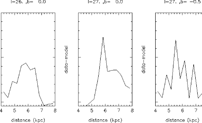
Figure 11: Histograms of distance distribution of the absolute difference ’data minus model’. Distance of data stars were derived using 12 x 12 bins of colour-magnitude with the following cuts: 12 $\leq$ K_s $<$ 13.5 and 1.6 $\leq$ J-K_s $<$ 3. for l=26^∘ b=0^∘, and 11.7 $\leq$ K_s $<$ 13. and 1.3 $\leq$ J-K_s $<$ 2.5 for l=27^∘ b=0^∘,-0.5^∘.

The distance distribution peaks very clearly at l=27^∘ b=0^∘, with a maximum at 5.9 kpc. The peak is lower but rather well defined at l=26^∘ b=0^∘ with the same maximum. At l=27^∘ b=-0.5^∘, the peak is ever less well defined, with a maximum at 5.5 kpc. We can thus deduce from these graphs that the stars of the excesses are located at a distance from the Sun a little lower than 6 kpc. This value confirms the result given by Hammersley et al. (2000).

6 Discussion

The Besançon model has shown good performances in producing the observed NIR counts at intermediate longitudes in the Galactic plane, where the disc is the major contributor, even if the vertical scalelength of the model components may have to be fine tuned.

We then confirm the existence of an overdensity between l=20^∘ and l=27^∘ in the Galactic plane, which seems to decrease inversely to the distance from the galactic plane at its end (l=26^∘-27^∘), and is located at a distance from the Sun a little lower than 6 kpc (assuming that they are disc-like stars).

The extension in longitude of the extra density and its confinement very close to the galactic plane may suggest an in-plane bar shape, as is argued in Hammersley et al. (2000) and López-Corredoira et al. (2001). Supposing that it does correspond to a bar, one can estimate its bar angle and its half-length, using the distance of excess stars from the Sun at its top end. Neglecting the width of the bar end and taking a distance between the Sun and the galactic center $R_{\odot}=8\pm 0.5$ kpc, and a distance from the Sun of bar stars $R=5.9\pm 0.5$ kpc, we obtain (see Figure 12) that the bar has a half-length $d=3.9\pm 0.4$ kpc and an angle from the Sun-center direction $\theta=45^{\circ}\pm 9^{\circ}$. These results are compatible with the values obtained in previous works: $d\approx 4$ kpc and $\theta\approx 43\deg$ (Hammersley et al., 2000). Moreover, other authors have given similar results for the geometrical parameters of the Galactic bar by using different methods. Sevenster et al. (1999) extracted an angle of 44^∘ for the bar through kinematic analysis of OH-IR stars. Nakai et al. (1992) studied the CO distribution in the inner Galaxy and suggested a bar near 45^∘, but with non-negligible uncertainties. More recently, Van Loon et al. (2003) studied luminosity distributions across the Galactic plane claimed for a bar with an orientation of 40^∘.

Figure 12: Scheme of the galactic in-plane bar

Unfortunately, if we can estimate bar parameters assuming as true the hypothesis that the excess stars belong to a bar population, the fact that the study was confined at l$\geq$15^∘ because of the completeness of data makes it impossible to confirm. Even the field at l=15^∘, very reddened and perhaps a little contaminated by the outer bulge, must be used with great care. Also, the most inner fields are dependent on the value of the disc hole scale length. Furthermore, the field at l=21^∘ b=0^∘, where the excess disappears, shows that the structure has inhomogeneities. On the other hand, extended star excesses can appear locally, close to rings for instance, without corresponding to a bar in term of dynamics.

New observations are needed to settle these uncertainties. If there is a bar, an excess of stars must exist at negative longitudes until the other end of the hypothetic bar. With a half-length of $3.9\pm 0.4$ kpc and an angle of $45^{\circ}\pm 9^{\circ}$, the bar far end stars would be located at the longitude l=-14${}^{\circ}\pm 2^{\circ}$ and at a distance from the sun of $11.1\pm 1$ kpc. Only much deeper data will allow us to detect them at these longitudes, and counts will be contaminated by the triaxial bulge in the inner regions. Moreover, kinematic measurements, at the top end of the hypothetic bar for instance, are necessary to know whether the extra density corresponds to a bar in term of dynamics or not. Such a study, using radial velocities, is being planned.

7 Acknowledgments

The TCS is operated on the island of Tenerife by the Instituto de Astrofísica de Canarias at the Spanish Observatorio del Teide of the Instituto de Astrofísica de Canarias.

References

- (1) Alves D.R. 2000, ApJ, 539, 732
- missing (2) Bahcall, J.N., & Soneira, R.M. 1980, ApJS, 44, 73
- Bienaymé et al. (1987) Bienaymé, O., Robin, A. C., & Crézé, M. 1987, A&A, 180, 94
- Cohen, Hammersley, & Egan (2000) Cohen, M., Hammersley, P. L., & Egan, M. P. 2000, AJ, 120, 3362
- De Jager & Nieuwenhuijzen (1987) De Jager, C., Nieuwenhuijzen, H. 1987, A&A, 177, 217
- (6) Eaton N., Adams D. J, Gilels A. B., 1984, MNRAS 208, 241
- Einasto (1979) Einasto, J. 1979, IAU Symp. 84, The Large Scale Characteristics of the Galaxy, ed. W.B. Burton, p. 451
- (8) Epchtein N. 1997, in: The Impact of Large Scale Near-IR Sky Surveys, F. Garzón F., N. Epchtein N., A. Omont, B. Burton, P. Persi, eds., kluwer, Dordrecht, p. 15
- missing (9) Garzón, F., Hammersley, P.L., Mahoney, T., et al. 1993, MNRAS, 264, 773.
- Garzon et al. (1997) Garzon, F., Lopez-Corredoira, M., Hammersley, P., Mahoney, T. J., Calbet, X., & Beckman, J. E. 1997, ApJ, 491, L31
- Garzon et al. (1999) Garz n F. 1999, in: The Evolution of Galaxies on Cosmological Timescales, ASP Conf. Ser. 187, ed. J. E. Beckman, & T. J Mahoney (Sheridan Books, S. Francisco), 31
- (12) Grocholski, A.J., Sarajedini, A. 2002, AJ, 123, 1603
- (13) Hammersley P. L., Garzón F., Mahoney T., Calbet X. 1994, MNRAS 269, 753
- (14) Hammersley, P.L., Garzon, F., Mahoney, T., & Calbet, X. 1995, MNRAS, 273 206
- Hammersley et al. (2000) Hammersley, P. L., Garzón, F., Mahoney, T. J., López-Corredoira, M., & Torres, M. A. P. 2000, MNRAS 317, L45
- Haywood et al. (1997) Haywood, M., Robin, A. C., & Crézé, M. 1997 A&A, 320, 440
- Lejeune et al. (1997) Lejeune, T., Cuisinier, F., & Buser, R. 1997 A&AS, 125, 229
- Lejeune et al. (1998) Lejeune, T., Cuisinier, F., & Buser, R. 1998 A&A, 130, 65
- López-Corredoira et al. (1999) López-Corredoira, M., Garzón, F., Beckman, J. E., Mahoney, T. J., Hammersley, P. L., & Calbet, X. 1999, AJ, 118, 381
- (20) López-Corredoira M., Hammersley P. L., Garzón F., Simonneau E., Mahoney T. J. 2000, MNRAS 313, 392
- missing (21) López-Corredoira, M., Hammersley, P.L., Garzón, F., Cabrera-Lavers, A., Rodríguez N., Schultheis, M., Mahoney T. J. 2001, A&A, 373, 139
- missing (22) López-Corredoira, M., Cabrera-Lavers, A., Garzón, F., Hammersley, P.L. 2002, A&A, 394, 883 (L02)
- Mathis (1990) Mathis, J.S. 1990 ARA&A 28,37
- missing (24) Nakai, N. 1992, PASJ, 44, L27
- missing (25) Paul, E.R. 1993, in The Milky Way Galaxy and Statistical Cosmology, 1890-1924 (Cambridge University Press, Cambridge).
- Reylé & Robin (2001) Reylé, C., Robin, A.C. 2001 A&A 373,886
- Robin & Crézé (1986) Robin, A. & Crézé, M. 1986, A&A, 157, 71
- Robin et al. (1996) Robin, A.C., Haywood, M., Crézé, M., Ojha, D.K., Bienaymé, O. 1996 A&A, 305,125
- Robin et al. (2000) Robin, A.C., Reylé, C., Crézé, M. 2000 A&A, 359,103
- Robin et al. (2002) Robin, A.C., Reylé, C., Derrière, S., Picaud, S. 2003 accepted by A&A
- Ruphy et al. (1996) Ruphy, S., Robin, A.C., Epchtein, N., Copet, E., Bertin, E., Fouqu é, F., Guglielmo, F. 1996 A&A, 313, 21
- (32) Sevenster, M., Saha, P., Calls-Gabaud, D., Fux, R. 1999, MNRAS 307,584
- (33) Skrutskie, M. F., Schneider S. E., Stiening R., et al. 1997, in: The Impact of Large Scale Near-IR Sky Surveys, F. Garzón F., N. Epchtein N., A. Omont, B. Burton, P. Persi, eds., kluwer, Dordrecht, p. 25
- (34) van Loon, J.T., Gilmore, G.F., Omont, A., Blommaert, J.A.D.L., et al. 2003, MNRAS, 338, 857
- (35) Wainscoat R. J., Cohen M., Volk K., Walker H. J., Schwartz D. E. 1992, ApJS 83, 111