Star formation rate indicators in the Sloan Digital Sky Survey

Abstract

The Sloan Digital Sky Survey (SDSS) first data release provides a database of $\approx 106000$ unique galaxies in the main galaxy sample with measured spectra. A sample of star-forming (SF) galaxies are identified from among the 3079 of these having 1.4 GHz luminosities from FIRST, by using optical spectral diagnostics. Using 1.4 GHz luminosities as a reference star formation rate (SFR) estimator insensitive to obscuration effects, the SFRs derived from the measured SDSS H$\alpha$, [Oii] and $u$-band luminosities, as well as far-infrared luminosities from IRAS, are compared. It is established that straightforward corrections for obscuration and aperture effects reliably bring the SDSS emission line and photometric SFR estimates into agreement with those at 1.4 GHz, although considerable scatter ($\approx 60\%$) remains in the relations. It thus appears feasible to perform detailed investigations of star formation for large and varied samples of SF galaxies through the available spectroscopic and photometric measurements from the SDSS. We provide herein exact prescriptions for determining the SFR for SDSS galaxies. The expected strong correlation between [Oii] and H$\alpha$ line fluxes for SF galaxies is seen, but with a median line flux ratio $F_{\rm[OII]}/F_{\rm H\alpha}=0.23$, about a factor of two smaller than that found in the sample of Kennicutt (1992). This correlation, used in deriving the [Oii] SFRs, is consistent with the luminosity-dependent relation found by Jansen et al. (2001). The median obscuration for the SDSS SF systems is found to be $A_{\rm H\alpha}=1.2\,$mag, while for the radio detected sample the median obscuration is notably higher, 1.6 mag, and with a broader distribution.

1 Introduction

The current star formation rate (SFR) of a galaxy is one of many important parameters used in developing our understanding of galaxy evolution. Various different indicators of galaxy SFR exist at different wavelengths, and include H$\alpha$ and [Oii] emission line luminosities, ultraviolet continuum luminosity, far-infrared (FIR) luminosity and radio luminosities (see reviews by Kennicutt, 1998; Condon, 1992). There are also strong suggestions that X-ray luminosity is an important SFR indicator (Grifiths et al., 1990; White & Ghosh, 1998; Ghosh & White, 2001; Ptak et al., 2001; Brandt et al., 2001; Georgakakis et al., 2003), although very faint X-ray observations are typically required to detect X-ray emission from star formation processes. In recent years several comparisons between different star formation indicators at varying wavelengths have been made, primarily establishing broad agreement between each but with detailed discrepancies and large scatter in the relations (Bell, 2003; Buat et al., 2002; Hopkins et al., 2001; Sullivan et al., 2001, 2000; Cram et al., 1998). One of the limiting factors in these comparisons to date is the mostly heterogeneous nature of the data being compared, and the relatively small numbers of objects investigated, no more than a few hundred.

The Sloan Digital Sky Survey (SDSS, Fukugita et al, 1996; Gunn et al., 1998; York et al., 2000; Hogg et al., 2001; Stoughton et al., 2002; Smith et al., 2002; Pier, 2003) eliminates these limitations. The SDSS is supplying the astronomical community with images and spectra providing an immense resource for use in numerous studies of galaxy, quasar, stellar and solar system properties. By identifying star-forming (SF) galaxies catalogued by the SDSS, a very large, homogeneous sample can be used to investigate the properties of star formation in galaxies. To support such studies, we investigate herein the consistency of SFRs derived from SDSS H$\alpha$ and [Oii] line measurements with those derived from the obscuration independent 1.4 GHz and FIR luminosities. Further, we empirically derive a non-linear calibration of SFR from the SDSS $u$-band luminosity, which gives SFR estimates highly consistent with the other four estimators. X-ray luminosities are not pursued here as an SFR estimator since not enough deep X-ray data is presently available for an exploration of a homogeneous X-ray detected SF galaxy sample. Results from an analysis of ROSAT All Sky Survey (RASS) identifications with SDSS galaxies in the early data release (Schulte-Ladbeck et al., 2003) confirm that almost all the RASS X-ray sources are identified with known galaxy clusters, quasars or active galactic nuclei (AGN).

In § 2 we describe the details of the current sample. The five SFR indicators are each explored in § 3, beginning with the 1.4 GHz estimator in § 3.1. The H$\alpha$ SFRs, including the obscuration and aperture corrections required, are presented in § 3.2. SFRs from [Oii], FIR and $u$-band luminosities are each given in §§ 3.3, 3.4, and 3.5 respectively. A discussion of the absolute SFR calibrations and the properties of the radio detected SF galaxies are explored in § 4. We summarise our results in § 5. Throughout this paper we assume a ($\Omega_{M}=0.3,\Omega_{\Lambda}=0.7,H_{0}=70$) cosmology.

2 Sample selection

The SDSS sample of spectroscopically observed main galaxies (Strauss et al., 2002) taken from the first data release (DR1, Abazajian et al., 2003) was used as the starting point for constructing our sample. This catalogue of $\approx 106000$ unique galaxies yields 3079 galaxies with 1.4 GHz measurements from the Faint Images of the Radio Sky at Twenty centimeters catalogue (FIRST, White et al., 1997). The radio identification from FIRST is based on positional matching within a radius of $1\farcs 5$ of the SDSS position (Ivezić et al., 2002). These galaxies form our primary sample for the investigations presented here.

Within our primary sample, we made use of three spectral diagnostic diagrams to classify galaxies as either SF, active galactic nuclei (AGN) or unclassified. Following Kewley et al. (2001) and Miller et al. (2003), the diagrams used were [Oiii]/H$\beta$ vs [Nii]/H$\alpha$, [Oiii]/H$\beta$ vs [Sii]/H$\alpha$, and [Oiii]/H$\beta$ vs [Oi]/H$\alpha$. We used the conservative requirements that for a galaxy to be classified as SF or AGN it had to be so classified in all three of the diagnostic diagrams, and remaining unclassified otherwise. Only emission lines where the measured flux was greater than twice the flux uncertainty (similar to a $2\sigma$ threshold) were considered in producing these classifications (Miller et al., 2003). Additionally, some objects could also be classified as AGN on the basis of having a large ratio of two emission lines for a given diagram, even though the other pair of lines for that diagram were not measurable (see discussion in Miller et al., 2003). Saturated emission lines will not affect our sample since saturated line parameters are not measured, so systems with saturated H$\alpha$, for example, can not be classified as SF galaxies. These systems are also extremely rare, and mostly dominated by nuclear emission from very nearby galaxies, so very few SF galaxies are likely to be omitted by excluding such objects. Our primary sample consists of 791 SF galaxies, 379 AGNs, 672 “quiescent” galaxies (with no measurable diagnostic emission lines), with the remaining 1237 galaxies either inconsistently classified, or lacking the required emission lines to be able to be classified in all three diagrams (see Figure 1). The ratio of AGN to SF systems is relatively high as a result of requiring radio detection (and hence a bias towards AGN systems) for inclusion in the sample. While a number of the “quiescent” galaxies are likely to be absorption line systems, typical of old stellar populations in elliptical galaxies, many are likely to be higher redshift objects whose emission lines fall below the sensitivity limits of the SDSS.

Although true absorption line systems, particular those at higher redshifts ($z\gtrsim 0.3$), will incorporate the luminous red galaxies (LRGs, Eisenstein et al., 2001), our sample has been defined to exclude these objects, being drawn from the main galaxy sample only (Strauss et al., 2002). This point is relevant since LRGs were noted by Ivezić et al. (2002) to have a relatively high fraction of radio counterparts. However, even if the LRGs are not excluded a priori, the results presented here do not change at all, since almost none of the LRGs satisfy our spectroscopic classification to be considered as SF galaxies.

Of the systems with the necessary emission lines, relatively few show conflicting classifications, as seen in Figure 1. The 177 galaxies inconsistently classified between AGN and SF may be composite systems hosting both types of activity (Hill et al., 2001), and are thus interesting in their own right, although they are not further investigated here.

All the classified SF and AGN galaxies have measurable H$\alpha$ luminosity ($L_{\rm H\alpha}$) and Balmer decrements, a result of requiring H$\alpha$ and H$\beta$ for classification, and we restrict the current investigation to the 791 galaxies classified as SF in all three spectral diagnostic diagrams. To calculate $u$-band luminosities we chose to use the Petrosian $u$-band absolute magnitudes, $M_{u}$, (calculated using the k-corrections of (Blanton et al., 2003)), treating them as AB magnitudes (Fukugita et al, 1996). Of the 791 SF systems, 752 have measurable [Oii] emission.

The completeness of the final spectroscopically classified sample is complex to define. The initial SDSS spectroscopic sample is complete to an optical flux limit corresponding to about $r=17.7$, and by requiring the presence of the [Sii] emission lines for classification, we implicitly impose an upper redshift limit of about $z=0.36$. By also requiring a 1.4 GHz detection from FIRST, we impose a second flux limit, this time corresponding to about 0.5 mJy. The full distributions in redshift, 1.4 GHz flux density and luminosity of the sample are presented in Figures 2 to 4. All three Figures show the distributions for the whole sample of 3079 galaxies, distinguishing the 379 AGNs, 791 SF, and 672 “quiescent” galaxies. The proportion of galaxies classified as “quiescent” becomes more dominant as redshift increases. This comes about as a combination of the detection limit of the survey and the necessary diagnostic emission lines moving out of the observable wavelength window. As a result, some galaxies classified as “quiescent,” especially those at higher redshifts, may not actually be quiescent at all. This is emphasised in Figure 4 where a large fraction of the brightest radio sources are classified as “quiescent.” In reality these systems may possess strong emission features that are below the detection threshold or lie outside the accessible SDSS window. The distribution in 1.4 GHz luminosities for the 3079 radio detections spans the very broad range from quite faint SF systems, $\log(L_{\rm 1.4\,GHz})\approx 20.5$, to powerful radio galaxies, $\log(L_{\rm 1.4\,GHz})\approx 26$ (compare with the range found by Sadler et al., 2002, for example). The luminosity range spanned by the spectroscopically classified AGNs is not too dissimilar from that of the SF systems, and this is a result of two effects: (1) requiring the presence of the necessary emission lines for the spectroscopic diagnostics limits the classified AGNs to lower redshifts, and hence lower luminosities; and (2) the more powerful AGNs may be dominated by elliptical type host galaxies, with absorption spectra.

Since the results of our SFR analysis do not rely on having a complete sample, and in order to retain the maximum number of objects for the analysis, we have chosen not to exclude any galaxies other than those required by our selection criteria above. Although our full spectroscopically classified sample thus remains incomplete at the higher redshift and lower flux density extremes, we can still define regimes over which our sample does approach completeness. The initial spectroscopic sample is known to be highly complete over the redshift range $0.05<z<0.1$ (Gómez et al., 2003). The flux density limit to which the FIRST survey is complete is about 2 mJy (White et al., 1997), so out to $z=0.1$, the 1.4 GHz detections should be complete above about $\log(L_{\rm 1.4\,GHz}/{\rm W\,Hz^{-1}})=22.5$ (corresponding, using the calibration described below, to SFR${}_{\rm 1.4\,GHz}\approx 20\,M_{\odot}\,$yr^-1). Despite this fairly high lower limit for completeness in SFR, the FIRST detections extend below the completeness limit to flux densities of about 0.75 mJy, allowing SFRs of order unity to be probed, although the radio detected sample at these levels is highly incomplete.

3 Star formation rates

Estimating a galaxy’s current SFR is typically done by applying a scaling factor to a star formation sensitive luminosity measurement for the galaxy (Kennicutt, 1998; Condon, 1992). Here we use this technique to estimate SFRs using H$\alpha$, [Oii], $u$-band, 1.4 GHz and FIR luminosities. In all the SFR calibrations given below we assume a Salpeter initial mass function (IMF) and a mass range from 0.1 to 100 $M_{\odot}$. Changing the mass range or choosing a different IMF will, of course, alter the values for the derived SFRs, and a discussion of these effects can be found in Kennicutt (1998). The radio luminosities have been calculated assuming a power-law spectral index $S_{\nu}\propto\nu^{-0.8}$ appropriate for galaxies dominated by synchrotron emission, and the optical luminosities are calculated by incorporating the k-corrections as measured by Blanton et al. (2003). Below we describe the details of calculating the SFRs for the five estimators we explore, and comparisons between each are performed.

3.1 1.4 GHz Star formation rates

Long-wavelength SFR estimates are insensitive to dust obscuration, increasing their attraction for SFR investigations, but they are not without limitations. Radio luminosity can be generated by AGN as well as star formation processes, and indeed the majority of apparently bright radio sources are AGN. By selecting for star formation directly from optical spectroscopic features, however, we have eliminated this potential source of confusion. The detailed physics involved in the connection between SF and radio emission, in addition, is still poorly understood, despite attempts by numerous models to explain it (e.g., Condon, 1992; Price & Duric, 1992; Chi & Wolfendale, 1990). Despite this, radio luminosities, in part because of the tight correlation with FIR luminosities (e.g., de Jong et al., 1985; Condon et al., 1991; Yun et al., 2001), appear to be robust and efficient SFR estimators (Condon, 1992; Cram et al., 1998; Bell, 2003). This, combined with the fact that the 1.4 GHz luminosity is insensitive to dust obscuration makes the use of SFR${}_{\rm 1.4\,GHz}$ very attractive, and we adopt this as a reference SFR when investigating the details of the other SFR measures. After the detailed investigation of the radio-FIR correlation by Bell (2003), we adopt the calibration derived therein between 1.4 GHz luminosity and SFR,

$${\rm SFR_{1.4GHz}}\,(M_{\odot}\,{\rm yr^{-1}})=\frac{fL_{\rm 1.4GHz}}{1.81\times 10^{21}\,{\rm W\,Hz^{-1}}},$$ (1)

where

$$f=\left\{\begin{array}[]{ll}1&L_{\rm 1.4GHz}>L_{c}\\ (0.1+0.9(L_{\rm 1.4GHz}/L_{c})^{0.3})^{-1}&L_{\rm 1.4GHz}\leq L_{c},\end{array}\right.$$ (2)

and $L_{c}=6.4\times 10^{21}\,$W Hz^-1. This calibration produces SFRs about a factor of two lower than the calibration of Condon (1992) for luminosities above $L_{c}$, while for fainter luminosities the SFRs progressively converge, with the present calibration eventually producing larger SFRs than that of Condon (1992) below about $3.4\times 10^{20}\,$W Hz^-1 (see discussion in Bell, 2003).

Most of the current generation of sensitive radio surveys, including FIRST, are conducted with interferometric telescopes, which, lacking short-spacing information, have a limited sensitivity to emission from more extended structures. The extent of this effect is dependent on the shortest baseline of the instrument. In particular, the FIRST catalogue starts losing sensitivity to 1.4 GHz emission for galaxies larger than about $10^{\prime\prime}$. For galaxies with a radius of $12^{\prime\prime}$ FIRST is only sensitive to about 84% of the emission, decreasing further for larger sources (Becker et al., 1995). If this effect is not accounted for, it can result in an apparent overestimate of the comparison SFR at low SFRs (see, for example, Figure 1 of Cram et al., 1998), although it is actually an underestimate in the 1.4 GHz derived SFRs. As shown in Figure 5, where the galaxy size is shown as a function of SFR${}_{\rm 1.4\,GHz}$ from FIRST, this starts becoming an issue in the current sample for galaxies with SFR${}_{\rm 1.4\,GHz}\lesssim 10\,M_{\odot}\,$yr^-1. To avoid such underestimates in SFR${}_{\rm 1.4\,GHz}$ for our analysis, we make use of the NRAO VLA Sky Survey (NVSS, Condon et al., 1998), a 1.4 GHz survey made with the VLA in the more compact D configuration. As a result of the compact VLA configuration used for the survey, the NVSS has poorer resolution than FIRST, but greater sensitivity to extended structure. It also has a survey limit similar to FIRST, and of the 107 SF galaxies in our sample with $r>10^{\prime\prime}$, 87 are present in the NVSS catalogue, within a $15^{\prime\prime}$ matching radius of the SDSS object (c.f. the $10^{\prime\prime}$ radius used by Sadler et al., 2002, for NVSS and 2dFGRS matches). These objects are shown in Figure 6, where the NVSS 1.4 GHz luminosities are compared with those from FIRST. For the systems larger than about $10^{\prime\prime}$ the extent of the underestimate in the FIRST measurements is clear. For all subsequent analysis herein, we use the NVSS derived SFRs in place of those from FIRST for galaxies with $r>10^{\prime\prime}$ to ensure no underestimates of 1.4 GHz derived SFR bias our results. Omitting the 20 objects with $r>10^{\prime\prime}$ and no NVSS measurement leaves a final sample of 771 SF galaxies.

3.2 H$\alpha$ Star formation rates

In estimating SFR from the H$\alpha$ luminosity we adopt the calibration given by Kennicutt (1998):

$${\rm SFR_{H\alpha}}\,(M_{\odot}\,{\rm yr^{-1}})=\frac{L_{\rm H\alpha}}{1.27\times 10^{34}\,{\rm W}}.$$ (3)

Prior to applying this calibration, though, there are several issues to address regarding the measurement of an H$\alpha$ luminosity representative of the full emission from a galaxy given a flux measurement from a fiber-based spectrum. These issues include both corrections for obscuration, due to the intrinsic dust content of the target galaxy, and aperture corrections, to account for the emission missed by virtue of the fiber diameter potentially being smaller than a target galaxy. Both these effects can be accounted for using the available SDSS data.

Before addressing these issues, we briefly digress to comment on the observing strategy called “smearing” (Stoughton et al., 2002). This is used in the SDSS to account for seeing and wavelength-dependent atmospheric refraction effects in ensuring the most accurate spectrophotometric calibration. A “smear-correction,” in brief, consists of scaling a primary spectrum so its smoothed continuum equals the smoothed continuum of a short exposure of the same object taken while the telescope pointing was dithered to cover a somewhat larger aperture than the fiber diameter. This scaling preserves line equivalent widths, but not line fluxes. The line fluxes are effectively being “aperture corrected” by scaling them assuming the line emission scales directly with the stellar continuum. This actually follows the same principle as the methods used below to perform aperture corrections, although the scaling of the smear-correction is to the stellar continuum within a fixed aperture for all galaxies, and will not necessarily encompass all of a target galaxy, especially at lower redshifts.

Naively using measurements of spectral line fluxes from smear-corrected spectra can thus potentially lead to small errors in the resulting fluxes and line ratios. Because of the fixed aperture effectively used in constructing the smear-correction, the line fluxes from smear-corrected spectra will be different from those constructed from the primary spectra with an aperture correction based on measured galaxy sizes or magnitudes. Some preliminary comparisons for line ratios, using Balmer decrement measurements in SF galaxies, quantify this small effect to some extent. Even with the Balmer decrement line ratio (widely spaced in wavelength) the systematic difference between primary and smear-corrected spectra is only about 10% at most.

In summary, equivalent widths measured from smear-corrected spectra should be consistent with those in primary spectra, and line ratios for lines close to each other in wavelength (such as the typical AGN/SF diagnostics) will be negligibly affected. But it is clear that to avoid potentially introducing small systematic offsets, the best solution for individual flux measurements, or line ratios widely separated in wavelength, is to use spectral line measurements made on spectra which have been processed without using the smear correction. All spectral line measurements used for the analysis herein were made on primary spectra, with no smear corrections applied.

3.2.1 Obscuration corrections

Galactic foreground obscuration is corrected for following Schlegel et al. (1998), but obscuration by dust intrinsic to the SF galaxies can cause more significant underestimates in the emission line and $u$-band derived SFRs. We address this by making obscuration corrections in two ways. All the SF classified galaxies have measured H$\alpha$ and H$\beta$ fluxes, so the Balmer decrement F_Hα/F_Hβ can be calculated, and used to estimate and correct for the obscuration. The suggestion of luminosity-dependent obscuration in SF galaxies (e.g., Hopkins et al., 2001; Sullivan et al., 2001), also recently identified in individual regions of star formation from spatially resolved spectroscopy of an extreme SF galaxy, IRAS 19254-7245 (Berta et al., 2003), is explored as well. New results from the Phoenix Deep Survey (Afonso et al., 2003) indicate, however, that the situation is more complex than implied by simple linear models. While galaxies with low SFRs seem to have relatively low levels of obscuration, at higher SFRs a broad range of obscurations are seen. A trend for an increase in the median obscuration with SFR, though, is still present. We make use of the method described by Afonso et al. (2003) and the relationship they derive to explore the effectiveness of such an empirical correction for the present sample, and perform an explicit comparison with the Balmer decrement correction.

Stellar absorption in the Balmer emission lines, if not accounted for, can cause a significant overestimation in the implied obscuration from measurements of the Balmer decrement (Rosa-González et al., 2002). Detailed analysis of continuum fitting to refine emission line measurements is being addressed by Tremonti et al. (2003), and an alternative line measurement method explored by Goto et al. (2003), but for the purposes of the current investigation it was deemed sufficient to assume a simple constant correction for stellar absorption in the measured Balmer line equivalent widths (EWs). The value of this equivalent width correction, ${\rm EW_{c}}$, for the H$\beta$ line was found by Miller & Owen (2002) to vary from about 1 Å for Sa galaxies to about 4 Å for extreme late types, with ${\rm EW_{c}}=2\,$Å for Sb galaxies, consistent with the typical value found in other studies of SF galaxies (e.g., Georgakakis et al., 1999; Tresse et al., 1996).

Given the broad range of possible stellar absorption values, the assumption of a common value may act to introduce a degree of scatter into the resulting SFR estimates. For the sample investigated here, the stellar absorption correction is typically a significant fraction of the measured H$\beta$ equivalent width, anything from a 10% to 100% correction. As a result, it is worth emphasising that the extent of the derived obscuration correction depends strongly on the assumed value of the stellar absorption. The assumption of a common value as done here should therefore be restricted only to studies of large samples where the gross characteristics of the population are being examined, and more refined measurements should be preferred for analyses of individual objects. Furthermore, since the relative correction is largest for systems with low EW, and since these tend to be those with higher luminosities, it is the bright galaxies that are most affected by any uncertainty in the extent of the absorption correction.

The EW correction is converted into a flux correction for the Balmer lines using

$$S=\frac{\rm EW+EW_{c}}{\rm EW}F,$$ (4)

where $S$ is the stellar absorption corrected line flux for H$\alpha$ or H$\beta$, EW is the equivalent width of the line, ${\rm EW_{c}}$ the correction for stellar absorption, and $F$ the observed line flux. The commonly assumed stellar absorption of ${\rm EW_{c}}=2\,$Å at H$\beta$ derives from a line measurement technique which involves an integration of the spectrum over a wavelength range encompassing the line (Miller & Owen, 2002; Goto et al., 2003). When alternative measurements are used, such as the Gaussian fitting of the SDSS pipeline, it appears that a smaller stellar absorption correction is necessary. This is a result of the SDSS spectral resolution, which partially resolves the stellar absorption, resulting in the fitted Gaussian being only incompletely diminished by the absorption. Thus the measured line flux (or EW) is larger than a flux-summing method would produce.

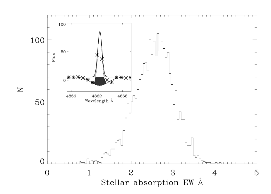
Figure 7: Histogram of intrinsic stellar absorption EWs at H$\alpha$ for the complete sample of SF galaxies. The median value is 2.6 Å. Inset: Sample SDSS spectrum indicating the effect of the pipeline measurement of the H$\beta$ emission line, illustrating the incomplete extent to which stellar absorption reduces the measured emission. The points are the actual measured SDSS spectrum. The solid line is the SDSS pipeline Gaussian fit to the emission, and the dashed lines are a double Gaussian fit, made by fixing an absorption component to have an EW$=3.0\,$Å the same EW as the absorption measured at H$\delta$ in this spectrum. The black shaded region indicates the true flux missed by the pipeline Gaussian fit in the measurement of the emission, while the grey shaded regions indicate excess flux added by the pipeline Gaussian fit. The black area minus the grey area is the true amount by which the pipeline fit underestimates the emission. It can clearly be seen that this area is smaller (by at least a factor of two) than the area of the stellar absorption component. Given a median stellar absorption of EW$=2.6\,$Å at H$\alpha$, the SDSS pipeline measurements, typically, are diminished by only about EW$=1.3\,$Å.

To establish the extent of this effect, the approximate distribution of actual stellar absorptions was first explored to determine the median absorption at the wavelength of H$\alpha$. Rather than simply assuming ${\rm EW_{c}}=2\,$Å for H$\beta$, we use the measured absorption at H$\delta$ in the SDSS spectra as a proxy for the H$\beta$ absorption. We then followed the prescription of Keel (1983) for deriving the stellar absorption at H$\alpha$, EW(H$\alpha$)$=1.30+0.40\,$EW(H$\beta$) (Miller & Owen, 2002). The resulting distribution of stellar absorption EWs at H$\alpha$ for a complete, volume limited sample of SF galaxies (constructed below, see § 3.5) is shown in Figure 7. The median value of this distribution is 2.6 Å, consistent with the observed range for late type galaxies. Since the resolution of SDSS spectra are sufficient to resolve this absorption, a correction smaller than this actual value needs to be applied. This is demonstrated explicitly for an actual SDSS spectrum in the inset of Figure 7. The SDSS pipeline Gaussian fit to the emission line underestimates the line flux by the black shaded area minus the grey shaded area, which can be seen to be smaller than the total stellar absorption, by at least a factor of two. Given the median stellar absorption of $2.6\,$Å, it seems that the appropriate stellar absorption correction should be at most about ${\rm EW_{c}}=1.3\,$Å. We adopt this value for the rest of this analysis.

Now, using the stellar absorption corrected Balmer line measurements, the Balmer decrement $S_{\rm H\alpha}/S_{\rm H\beta}$ can be constructed. The obscuration correction is then derived using the Balmer decrement and an obscuration curve. For making obscuration corrections to the emission lines, we use the Milky Way obscuration curve of Cardelli et al. (1989) as referenced in Table 2 of Calzetti (2001). For the obscuration corrections to the stellar continuum in the $u$-band (§ 3.5), we use the obscuration curve of Calzetti et al. (2000) derived for starburst galaxies. Note that the extent of the obscuration experienced by emission lines and the stellar continuum at the same wavelength differs by a factor of about two (Calzetti, 2001).

The stellar absorption corrected Balmer decrements are shown as a function of SFR_1.4GHz in Figure 8. The predicted Balmer decrement from the SFR-dependent obscuration of Afonso et al. (2003) is shown as the solid line in this Figure, and that of Hopkins et al. (2001) as the dashed line. The relation independently derived by Sullivan et al. (2001) lies $10\%$ higher than that of Hopkins et al. (2001), while having an almost identical slope. These relations have been converted to the current SFR calibrations and cosmologies where necessary. As discussed by Afonso et al. (2003), the empirical relation found by Hopkins et al. (2001) appears to be affected by sample selection effects (being restricted to higher EW systems). This results in a model that provides a reasonable approximation for larger EW systems (EW(H$\alpha$)$\gtrsim 70$ Å), but is clearly an underestimate for smaller EW systems. For the whole sample, the model of Afonso et al. (2003) is better at tracing the trend in the median obscuration with SFR, although appears to be a slight overestimate. This is discussed further in § 3.2.3 below. Again, very importantly, there is significant scatter in the distribution of actual Balmer decrements about such trends, particularly at high SFR.

On top of the overall trend for systems with higher SFRs to have a higher median Balmer decrement, the observed trend with EW in Figure 8 is also likely to be real, and not merely an artifact of the chosen stellar absorption correction. In the relatively low SFR range $1<{\rm SFR_{1.4GHz}}<10\,M_{\odot}\,$yr^-1, for example, the systems with EW$<70\,$Å have a median Balmer decrement of 6.1, compared with 5.3 for the systems with larger EWs. If the stellar absorption correction was boosted as high as ${\rm EW_{c}}=2.6\,$Å, (an unreasonably large estimate given the illustration in Figure 7), these median values decrease only to 5.4 and 4.6 respectively. This indicates both that there are real differences in the extent of the typical absorption, depending on the observed EW, and that this difference is not an artifact of the chosen stellar absorption correction. The extent of the absorption, moreover, is not negligible, even at these relatively low SFRs.

3.2.2 Aperture corrections

In addition to the obscuration correction, the emission line luminosities also require an aperture correction to account for the fact that only a limited amount of emission from a galaxy is detected through the $3^{\prime\prime}$ diameter fiber. For both the H$\alpha$ and [Oii] emission lines, this is done as follows.

The H$\alpha$ EW (corrected for stellar absorption) can be used along with an estimate of the continuum luminosity for the galaxy from the photometric catalogue at the observed wavelength of H$\alpha$, to recover an effective H$\alpha$ line luminosity for the whole galaxy. Explicitly, (before obscuration corrections are applied),

$$L_{\rm H\alpha}\,({\rm W})=({\rm EW+EW_{c}})\,10^{-0.4(M_{\rm r}-34.10)}\,\frac{3\times 10^{18}}{(6564.61(1+z))^{2}}$$ (5)

where $M_{\rm r}$ is the k-corrected absolute $r$-band AB-magnitude, derived from the observed $r$-band Petrosian magnitude. The last term converts this luminosity from units of W Hz^-1 to W Å^-1. This Equation assumes that the flux of the continuum at the wavelength of H$\alpha$ can be represented by the flux at the effective wavelength of the $r$-band filter ($\approx 6222\,$Å). While this is not strictly true, the continuum in these SF systems in the wavelength range of interest is flat enough that it is a good approximation. A more refined estimate can be made using an interpolation between the absolute magnitudes in the $r$ and $i$, or $i$ and $z$ filters, as appropriate for the redshift of the galaxy. This was explored and found to make a negligible difference in the resulting distribution of SFRs and in the comparison with SFRs estimated at other wavelengths.

The aperture correction implicitly assumes that the emission measured through the fiber is characteristic of the whole galaxy, and that the SF is uniformly distributed over the galaxy. Issues such as galaxy orientation and patchy distributions of SF regions, primarily when the aperture corrections are large, will increase the uncertainties in this form of aperture correction estimate.

In the case of the [Oii] luminosity, an exactly analogous method is used to calculate the aperture correction, although no stellar absorption correction is necessary for the EW of [Oii]. In Equation 5 $M_{\rm u}$ is substituted for $M_{\rm r}$, and the wavelength of [Oii], 3728.30 Å, is used in place of that of H$\alpha$, 6564.61 Å, in the last term. The explicit calculation used in constructing the final SFR_Hα, incorporating both the aperture correction and the obscuration correction, is given as Equation B2 in Appendix B.

An alternative method of applying an aperture correction is described in Appendix A, along with a fuller discussion of systematic uncertainties and an exploration of how the aperture correction depends on parameters such as angular size and redshift.

3.2.3 Comparison with 1.4 GHz SFRs

The estimated SFRs derived from H$\alpha$ luminosities are shown as a function of SFR${}_{\rm 1.4\,GHz}$ in Figure 9. Each step in the process of calculating the H$\alpha$ luminosities is shown, to emphasise the magnitude of each effect. The uncorrected SFRs shown are calculated directly from the H$\alpha$ line luminosities prior to any obscuration or aperture corrections. The aperture corrected SFRs are calculated from the luminosities obtained using Equation 5 before applying obscuration corrections, and finally, from Equation B2 incorporating the obscuration correction as well. It can be seen that, on average, the combined effect of the aperture and obscuration correction is to increase uncorrected luminosities (and SFRs) by a factor of about 20. The resulting estimates from H$\alpha$ and 1.4 GHz luminosities are highly consistent, although there remains a significant amount of scatter. The rms characterising the extent of this scatter, in the sense of the rms deviation from the one-to-one line, is 0.21 dex, or about a factor of 1.6 either side of the line. The extrema of the scatter (apart from a small number of significant outliers) span about 1 dex.

The results of using the obscuration correction method of Afonso et al. (2003) are also shown in Figure 9, producing a similar distribution for the derived H$\alpha$ SFRs as the Balmer decrement correction. Directly comparing SFR_Hα estimated using obscuration corrections derived from the Balmer decrement with those using the method of Afonso et al. (2003) show that the relation of Afonso et al. (2003) gives, on average, an overestimate of about 20%. This is not unexpected given the location of the trend shown in Figure 8. Afonso et al. (2003) discusses the fact that this relation, derived from a radio-selected sample of SF galaxies, reflects the presence of galaxies with larger obscurations, able to be detected in radio-selected samples, and possibly overlooked in UV or optically selected samples. This point will be discussed in more detail in § 4.2 below. In any case, for this type of application empirical relations like that of Afonso et al. (2003) and Hopkins et al. (2001), when their selection effects and limitations are correctly taken into account, appear to be useful tools for estimating obscuration corrections in the absence of more physical measurements.

It is possible that some of the scatter observed in Figure 9 may be produced by our assumption of a common stellar absorption correction. This was investigated by applying corrections using the individual estimates derived above, from the method of Keel (1983). No measurable reduction in the resulting scatter was detected, suggesting that the assumption of a common EW correction for stellar absorption does not dominate the observed scatter in these results. To account for the scatter, other physical processes must be investigated.

The differences between the measurements of SFR from H$\alpha$ and 1.4 GHz luminosities from Figure 9(c) were further investigated to explore whether there was any residual trend in the relation. Figure 10 shows the ratios of these SFRs as a function of redshift, indicating the consistency of the two measurements, on average. The effect of the flux density limit of the radio survey is also shown. This limit (about 0.75 mJy, somewhat lower than the completeness level of 2 mJy) starts to bias the observed distribution for systems beyond a redshift of $z\approx 0.1$. This bias is in the sense of losing sensitivity to systems with apparent underestimates of SFR${}_{\rm 1.4\,GHz}$ with respect to SFR_Hα. Also, below a redshift of $z\approx 0.03$, the distribution seems to show predominantly more systems with SFR_Hα overestimated compared to SFR${}_{\rm 1.4\,GHz}$. This is unlikely to be a selection effect, and is also unlikely to be an underestimate in the 1.4 GHz luminosities, as the NVSS measurements used for these large, nearby systems are sensitive to the emission over the full range of sizes seen. This effect is instead more likely to be an overestimate in the H$\alpha$ luminosities as a result of the effective aperture correction used. The aperture correction implicitly assumes that the star formation sampled through the fiber is representative of the distribution over the whole galaxy, and that this scales directly with the broadband optical emission. The more realistic scenario is that (especially in relatively low SFR, nearby systems) the star formation is patchy, and distributed non-uniformly throughout the galaxy. Hence it is not surprising that the simple aperture correction used for these systems produces an overestimate. This overestimate is not seen in the distribution of measurements between $0.05\lesssim z\lesssim 0.1$, where the 1.4 GHz flux density limit does not yet affect the observed distribution. The most likely explanation here is that the lowest redshift systems have a larger contribution from galaxies with centrally concentrated star formation, and possibly also from irregular and dwarf systems, known to contain patchy SF distributions.

It is worth pointing out here that there is a subtle selection effect arising from the requirement of having a radio detection for the SF sample. This is an effective emission line flux limit resulting from the radio flux density limit. If the 1.4 GHz detection limit of about 0.75 mJy is transformed to an H$\alpha$ flux limit via the SFR calibrations of Equations 1 and 3, (after incorporating the factor of 20 corresponding to the average combined obscuration and aperture correction), an effective H$\alpha$ flux limit of about $3.5\times 10^{-18}\,$Wm^-2 is derived. This is over an order of magnitude higher than the minimum observed H$\alpha$ fluxes of $\approx 3\times 10^{-19}\,$Wm^-2 for the spectroscopically classified SF galaxies in the whole DR1. A similar relation can be derived for [Oii] line fluxes. In this case the effective [Oii] flux limit ($\approx 7\times 10^{-19}\,$Wm^-2) imposed by the radio flux density limit is a little closer to the actual minimum [Oii] fluxes observed ($\approx 1\times 10^{-19}\,$Wm^-2) in the DR1 SF galaxies. The primary result of this selection effect seems to be that the radio detected sample is more similar to a complete sample, in the sense that the incompleteness at low H$\alpha$ fluxes is removed. This is explored further in § 4.2.

3.3 [Oii] Star Formation Rates

An SFR calibration based on the [Oii] emission is an important tool for probing galaxy SFRs at $z\gtrsim 0.4$ where H$\alpha$ is redshifted out of the bands easily accessible by optical spectroscopy. As with H$\alpha$, [Oii] luminosities require aperture and obscuration corrections, which are described in detail in § 3.2 above. SFRs derived from [Oii] luminosities are based on the fact that there is a good correlation between observed [Oii] line fluxes and observed H$\alpha$ lines fluxes (i.e., prior to any obscuration corrections). The SFRs come from using the [Oii] emission as a proxy for the H$\alpha$ emission, which must then be corrected for obscuration based on the obscuration at the wavelength of H$\alpha$ in order to use the SFR calibration derived for H$\alpha$ luminosities (Kennicutt, 1998, 1992).

Many recent estimates of [Oii] SFRs rely on the SFR calibration of Kennicutt (1998), an average of the calibrations reported by Gallagher et al. (1989) and Kennicutt (1992), each of which are based on samples of fewer than 100 galaxies. In particular the observed ratio $F_{\rm[OII]}/F_{\rm H\alpha}=0.45$ from Kennicutt (1992) is extensively used. This ratio is, however, luminosity and metallicity dependent (Jansen et al., 2001), and the appropriate ratio should be determined for a given sample depending on its selection effects. The current sample of 791 SDSS SF galaxies with radio counterparts includes 752 with measured [Oii] emission. Following the methodology used in Kennicutt (1992), the ratio of the observed fluxes in the [Oii] and H$\alpha$ emission lines was investigated (see also Figure 20, and subsequent discussion in § 4.2), and the median ratio was found to be $F_{\rm[OII]}/F_{\rm H\alpha}=0.23$. (This result comes after a stellar absorption correction EW${}_{\rm c}=1.3\,$Å is applied to the H$\alpha$ emission, although the median ratio changes negligibly if this step is omitted.)

Applying or omitting the aperture corrections when calculating this ratio also changes the median value negligibly, although it is certainly true that a differential distribution for the origin of the line emission would not be accounted for with the aperture correction methods used here. If [Oii] emission came predominantly from galaxy disks, and H$\alpha$ predominantly from galaxy nuclei, for example, the current estimate would be skewed low. It seems unlikely, though, that this contrived geometry of line emission should occur for the majority of systems. Given, additionally, the expected association of both forms of emission with star formation regions, it seems reasonable that both [Oii] and H$\alpha$ emission should be at least approximately colocated throughout SF galaxies.

The median ratio determined for the current sample (from fiber spectroscopy) is slightly lower than that found by Jansen et al. (2001) (using spatially integrated spectra) for galaxies of similar absolute magnitude. This does not appear to be an artifact of the radio selected nature of the current sample. If the radio detection requirement is relaxed, and a complete, volume-limited sample of optically selected SF galaxies constructed, an unbiased estimate of the distribution of this flux ratio can be established. This is pursued further in § 4.2 below, and results in median values for $F_{\rm[OII]}/F_{\rm H\alpha}$ very similar to that found for the full radio detected sample currently being explored. For the present discussion we adopt the ratio $F_{\rm[OII]}/F_{\rm H\alpha}=0.23$ as being representative of typical SF galaxies, given the optical luminosity range of the present sample. This calibration may also be useful for higher redshift surveys of galaxies of similar luminosity, where observations of the H$\alpha$ line are more difficult. The metallicity dependence of the $F_{\rm[OII]}/F_{\rm H\alpha}$ ratio, however, must also be accounted for at higher redshifts, given the strong evolution in the metallicity-luminosity relation (Kobulnicky et al., 2003).

Using this estimate for the correlation between [Oii] and H$\alpha$ line fluxes the calibration of $L_{\rm H\alpha}$ to SFR (Equation 3) is transformed to

$${\rm SFR_{\rm[OII]}}\,(M_{\odot}\,{\rm yr^{-1}})=\frac{L_{\rm[OII]}}{2.97\times 10^{33}\,{\rm W}},$$ (6)

where $L_{\rm[OII]}$, due to the way this calibration was derived, must incorporate the obscuration correction valid at the wavelength of H$\alpha$ (Kennicutt, 1998). The final [Oii] SFR estimate is explicitly shown in Appendix B as Equation B5.

The effectiveness of this calibration can be seen in the comparison of [Oii] derived SFRs with those from 1.4 GHz and H$\alpha$ in Figure 11. The small number of systems in Figure 11(a) with anomalously high 1.4 GHz SFRs may be composite AGN/SF systems, in which the AGN is masked by obscuration at optical wavelengths, since the H$\alpha$ and [Oii] SFRs for these systems are in good agreement.

3.4 FIR Star Formation Rates

FIR flux densities are available from the IRAS catalogs for a sub-sample of our SF galaxies, and positional matching with the FIRST radio sources identifies 191 galaxies in this final SF sample with IRAS detections. The $60\,\mu$m and $100\,\mu$m flux densities, $S_{60}$ and $S_{100}$ can be used to derive a FIR flux following Helou et al. (1988), FIR(W m^-2)$=1.26\times 10^{-14}(2.58\,S_{60}+S_{100})$. There are several calibrations of FIR luminosity to SFR in the literature, (for a summary see Kennicutt, 1998). We begin with the recent calibration of Bell (2003), (from which our chosen 1.4 GHz SFR calibration was derived):

$${\rm SFR_{FIR}}\,(M_{\odot}\,{\rm yr^{-1}})=\frac{1.75fL_{\rm FIR}}{2.44\times 10^{36}\,{\rm W}}=\frac{fL_{\rm FIR}}{1.39\times 10^{36}\,{\rm W}},$$ (7)

where

$$f=\left\{\begin{array}[]{ll}1+\sqrt{2.186\times 10^{35}\,{\rm W}/L_{\rm FIR}}&L_{\rm FIR}>L_{c}\\ 0.75\,(1+\sqrt{2.186\times 10^{35}\,{\rm W}/L_{\rm FIR}})&L_{\rm FIR}\leq L_{c},\end{array}\right.$$ (8)

and $L_{c}=2.186\times 10^{37}\,$W. $L_{\rm FIR}$ is the luminosity corresponding to the FIR flux as defined above, and the factor of 1.75 in Equation 7 converts this to a luminosity representative of the full ($8-1000\,\mu$m) mid- to far-infrared spectrum (for details see Bell, 2003; Kewley et al., 2002). The piecemeal nature of this Equation comes from the assumption of varying fractions of old stellar populations with luminosity. It is plausible, however, that galaxies with high FIR luminosities in the current sample have similar relative contributions (to FIR luminosity) from old stellar populations as the lower luminosity systems. This is in contrast to the sample from Bell (2003), which was more inhomogeneously constructed, possibly resulting in preferential selection of starbursting galaxies with low old fractions above $10^{11}\,M_{\odot}$ yr^-1 (Bell, 2003, private communication). Consequently we have chosen to adopt an old stellar population fraction of 30% independent of luminosity, and apply the portion of Equation 8 valid for $L_{\rm FIR}\leq L_{c}$ to all galaxies. This is explicitly presented in Equation B10. We further recommend this strategy to others working on samples of radio-selected galaxies (Bell, 2003, private communication). The resulting SFR_FIR is compared with those from 1.4 GHz and H$\alpha$ in Figure 12. This calibration is within a factor of two of that of Kennicutt (1998) down to about $3\times 10^{-3}\,L_{c}$ (Bell, 2003). Note that the empirical relation from Buat & Xu (1996), measured from a sample of galaxies of types Sb and later, produces SFRs almost 80% larger than this calibration, and that of Condon (1992) produces SFRs about $60\%$ larger.

3.5 $u$-Band Star Formation Rates

While ultraviolet (UV) luminosity ($\lambda\lesssim 2500\,$Å) is commonly used as an SFR indicator, the luminosity at $u$-band wavelengths ($\lambda\approx 3600\,$Å) is similarly dominated in starburst galaxies by young stellar populations, and in the absence of UV measurements the $u$-band luminosity may thus be used instead as an SFR indicator (Cram et al., 1998). The $u$-band luminosities used here are derived from the SDSS k-corrected absolute $u$-band magnitudes (Blanton et al., 2003), after incorporating an obscuration correction based on the Balmer decrement and the extinction curve from Calzetti et al. (2000). It is worthwhile pointing out that the average $u$-band obscuration correction ranges from a factor of 3 at SFRs of $1\,M_{\odot}\,$yr^-1 up to about a factor of 10 at SFRs of $100\,M_{\odot}\,$yr^-1.

UV luminosities have been extensively used as SFR indicators, and for wavelengths $1500\,$Å $\lesssim\lambda\lesssim 2500\,$Å the calibration given by Kennicutt (1998)

$${\rm SFR_{UV}}\,(M_{\odot}\,{\rm yr^{-1}})=\frac{L_{\rm UV}}{7.14\times 10^{20}\,{\rm W\,Hz^{-1}}}$$ (9)

has proven quite effective. For $u$-band luminosities, though, it is somewhat more difficult to assign a simple scaling factor to derive an SFR due to the strong dependence on the evolutionary timescale. From synthetic galaxy spectra (e.g., Fioc & Rocca-Volmerange, 1997) it can be seen that the $u$-band luminosity varies from about factor of 10 lower than the UV luminosity at the onset of a burst of star formation, to almost equivalent by $10^{8}$ years later (see also discussions of the dependence of UV measures on the timescale of SFR in Sullivan et al., 2000; Glazebrook et al., 1999).

Given this sensitivity of the $u$-band (and indeed UV) luminosity to the starburst age and the assumed star formation history, a more complex calibration is in general likely to be necessary. This may take the form of a non-linear dependency on $L_{\rm U}$ to reflect the rapid change of $L_{\rm U}$ with respect to $L_{\rm UV}$ during the first $10^{8}$ years of a starburst, and to account for the presence of old stellar populations that are likely to contribute significantly to $L_{\rm U}$ in less luminous systems (Bell, 2003). More quiescent or low-luminosity SF systems have a relatively larger contribution to their $u$-band luminosity from old stellar populations, (they are, on average, redder than more luminous galaxies), and this causes a linear calibration from luminosity to SFR to result in an overestimate of the SFR. While these effects can be modelled in detail using stellar spectral synthesis methods (Sullivan et al., 2000), for the purposes of a simple SFR estimate based on a measured luminosity an empirical non-unity power-law relationship between $u$-band luminosity and SFR can be derived. Although providing no information about the SFR history or the SED evolution, such a calibration has the advantage of being easy to construct and can form a useful tool in subsequent analysis.

To construct such a tool we require a complete, volume-limited sample of galaxies, a necessity not demanded of the previous sections where straightforward comparisons between existing calibrations were being explored. This requirement is necessary to avoid biasing the calibration low or high based on the independent limits of the H$\alpha$ and $u$-band detections. In order to have the largest complete sample from which to derive the new calibration, and to eliminate any potential concerns introduced regarding radio selection, we thus construct an SF galaxy sample from the DR1 based on the completeness criteria described by Gómez et al. (2003), and do not require radio detection at all. The criteria used specify that galaxies should lie closer than $z\leq 0.095$ (since aperture corrections are applied, no lower redshift limit is necessary) and have $M_{\rm r}\leq-20.57$ (after converting to our chosen value of $H_{0}$). The small number of systems with $z<0.05$ (the lower redshift limit used by Gómez et al., 2003) which show slight overestimates in their aperture corrected SFR_Hα relative to SFR_1.4GHz do not bias the result, which remains unchanged if these objects are excluded. A further restriction was applied, a limit on the H$\alpha$ fluxes, $F_{\rm H\alpha}>3\times 10^{-18}\,$Wm^-2. This corresponds to an SFR of about $0.5\,M_{\odot}$yr^-1 at the redshift limit of the complete sample, and ensures no bias will be introduced to the derived calibration through the presence of incompletely sampled fainter H$\alpha$ systems. This results in a sample of 2625 spectroscopically classified SF galaxies with measured H$\alpha$ and $u$-band luminosities.

Using this sample the ordinary least-squares bisector method of linear regression (Isobe et al., 1990) was applied to $\log(L_{\rm U})$ (after applying obscuration corrections based on the Balmer decrements) and $\log({\rm SFR_{H\alpha}})$. It is recognised that the luminosity limits imposed by requiring completeness will cause a small bias to this fit, (since the imposed limit on $r$-band luminosity translates to an effective limit on $u$-band luminosity, and omitting galaxies with lower luminosities affects the slope of the fit slightly), nevertheless this still produces a better estimate of the true relation than were an incomplete sample used. The comparison for the complete sample of galaxies between $L_{\rm U}$ and SFR_Hα can be seen in Figure 13(a), which indicates the resulting best fit relation. This relation results in the calibration:

$${\rm SFR_{U}}\,(M_{\odot}\,{\rm yr^{-1}})=\left(\frac{L_{\rm U}}{1.81\times 10^{21}\,{\rm W\,Hz^{-1}}}\right)^{1.186},$$ (10)

and the result of applying this calibration is shown in Figure 13(b). Strictly speaking, this calibration is only valid over the range of luminosities probed here, $2\times 10^{21}\lesssim L_{U}\lesssim 10^{23}\,$W Hz^-1. The explicit calculation in terms of the observable quantities is given in Equation B8, in Appendix B. Since the calibration from luminosity to SFR is no longer linear, a multiplicative obscuration correction cannot be applied directly to the SFR in the same manner as to the luminosity. Rather the appropriate exponent as given in the SFR calibration must be incorporated as well.

The entire sample of 21649 SF galaxies with measured $u$-band and H$\alpha$ SFRs are compared in Figure 14. The effects of the incompleteness can be seen, appearing as a slight apparent bias to overestimated $u$-band SFRs. The fitted relation, therefore, is sensitive to the completeness of the sample being used, emphasising the need for the initial calibration to be performed on a well-defined sample.

Using the new SFR calibration for $u$-band luminosity, SFR_U is shown as a function of SFR${}_{\rm 1.4\,GHz}$ in Figure 15. The rms deviation between SFR_U and SFR${}_{\rm 1.4\,GHz}$ is 0.23 dex, or a factor of 1.7 either side of the one-to-one line.

4 Discussion

4.1 Systematics and absolute SFR calibrations

We have demonstrated a consistency between independent SFRs estimated from H$\alpha$ and 1.4 GHz luminosities, used an observed H$\alpha$/[Oii] flux correlation to establish the consistency of the [Oii] SFRs, identified the FIR calibration giving most consistent SFRs, and derived a $u$-band calibration defined to give consistent SFRs. It should be emphasised that, since the calibration for SFR${}_{\rm 1.4\,GHz}$ is derived from the FIR calibration (Bell, 2003), and since the [Oii] and $u$-band calibrations are derived from the H$\alpha$ calibration, the only independent calibrations being directly compared are those of H$\alpha$ and FIR, both ultimately coming from Kennicutt (1998). This is still non-trivial, however, given the different physics involved in the two derivations (ionising luminosities compared with total bolometric fluxes), and the broad consistency seen across the range of wavelengths explored is highly encouraging. This consistency is in spite of the large scatter, frequently referred to above, in the SFR values measured at different wavelengths for individual systems. The dispersions about the one-to-one line for each estimator compared with the 1.4 GHz estimator are summarised in Table 1, where the uncertainties shown are the rms deviations either side of the one-to-one line. Some issues that are likely to contribute to this observed scatter include (1) the reliability of the assumptions underlying the aperture corrections to the emission line estimates; (2) whether the Balmer decrement obscuration estimate (which is measured only for the region seen through the fiber aperture) is valid for the whole galaxy; (3) the extent to which any low luminosity AGN that may be present in the SF galaxies contributes to the observed radio luminosity; (4) galaxy to galaxy differences in the average 1.4 GHz luminosity generated by supernovae, either through differences in electron population densities, temperatures, or confinement, strength of interstellar magnetic fields, or other physical differences.

It is possible that in addition to this observed scatter, however, the absolute SFR calibrations are still uncertain by up to a factor of two (Bell, 2003; Condon, 2002). Apart from concerns arising through the detailed physics involved in deriving the SFR calibrations, the only additional systematics that might change the quantitative SFRs derived herein are the assumed equivalent width correction to account for stellar absorption, and the chosen obscuration curve. The aperture corrections could produce underestimates of SFR_Hα only for galaxies large enough that the fiber predominantly samples light from the nucleus, the star formation occurs primarily in the disk, and the galaxy is observed close to face on. Hence it seems likely that any bias caused by the aperture corrections will be overestimates of SFR_Hα, as seen in Figure 10, and that these are relatively small effects restricted to very nearby systems. (It is of course possible that the assumptions involved in making the aperture correction contribute, perhaps significantly, to the scatter seen in the measured individual SFRs.)

Differences between estimates of the obscuration curve appropriate for correcting emission lines produce only small changes (of order $5\%$) from the results given here. The assumption of Case B recombination may also contribute to the scatter between the different SFR estimates, since this will not be valid for all systems (although it should be reasonable for the majority of the SF galaxies). It is also possible that the detailed geometries of gas and dust in individual objects could result in quite different obscurations than estimated here, but for this sample of relatively low redshift galaxies the obscuration curve adopted should be fairly representative. These effects, while contributing to the observed scatter, should not act in a systematic fashion.

The H$\alpha$ SFR values reported here could potentially be increased by up to about $20\%$ by reducing the chosen EW correction for stellar absorption (a value of ${\rm EW_{c}}=0.7\,$Å increases the derived SFRs by this factor). This arises through the change introduced in the Balmer decrement when a different value of the ${\rm EW_{c}}$ is used. Since the measured H$\beta$ emission is in many cases comparable to the correction being applied to it, the resulting Balmer decrement is very sensitive to the chosen value. Values of ${\rm EW_{c}}$ smaller than about 0.7 Å would, however, no longer be consistent with the stellar absorption corrected Balmer decrements derived from the flux-summing method of line measurement. Making the stellar absorption correction smaller also increases the discrepancy between the two methods (described in Appendix A) of estimating SFR_Hα. So there is a limit of about $20\%$ by which SFR_Hα can be increased through the chosen estimate of ${\rm EW_{c}}$. Even in combination with the other systematic uncertainties in the H$\alpha$ SFR calibration, the values reported here seem reliable in an absolute sense to better than a factor of two. In any case, it doesn’t seem to be possible to produce high enough values of SFR_Hα to become consistent with the 1.4 GHz SFR calibration of Condon (1992) (which gives SFRs about a factor of two higher than the calibration used here), without revising the H$\alpha$ SFR calibration.

Since the SFR_[OII] calculation uses the same obscuration correction as for H$\alpha$, and since the $u$-band SFRs are calibrated to SFR_Hα, these would both be changed consistently as different estimates of ${\rm EW_{c}}$ change SFR_Hα in the above case. The FIR estimate, similarly, is consistent with the chosen 1.4 GHz estimate (by construction), so the only truly independent SFR estimators in the current investigation are SFR_Hα and SFR_1.4GHz. The consistency between these two results does, however, support the reliability of the assumed stellar absorption correction, and since the absolute calibration of the H$\alpha$ SFRs appears quantitatively reliable, to better than a factor of two, the radio and FIR calibrations adopted must be similarly reliable. This conclusion regarding the quantitative reliability of the SFR calibrations, of course, only applies to the overall population. Measurements of individual objects, as can be seen from the large scatter in all the SFR comparison diagrams, can still easily be uncertain by factors of two or more.

So, despite the discrepancies (factors of two) in many of the available calibrations, a strong argument can be made that the absolute SFR calibrations should be close to those adopted here. This preliminary exploration suggests that the presently adopted calibrations give SFRs which are on average reliable to better than a factor of two.

4.2 Radio-selected SF galaxies

The properties of the radio detected SF galaxies have been explored to investigate some details of how they differ from optically selected SF galaxies. The complete sample of SF galaxies constructed for the $u$-band calibration in § 3.5, above, was used to compare the distribution of various measured parameters between the optically selected and radio detected objects. There are 2625 galaxies in the complete sample, of which 380 are radio detected. Figure 16 indicates the distribution in optical luminosity spanned by both the complete sample and the radio detected galaxies within that sample. The median magnitudes of these two distributions are similar ($-20.6$ for the complete sample, $-20.8$ for the radio detected systems), although the radio detected systems show a much broader magnitude distribution. Gaussian fits to the two histograms indicate a full width at half maximum (FWHM) of 0.9 mag for the complete sample, and 1.3 mag for the radio detected galaxies. Figure 17 shows the distributions of rest frame $u-g$ and $u-r$ colors, concentration index inverse, $1/c$, and D₄₀₀₀ for both the complete SF sample and the radio detected galaxies in the complete sample. (Concentration index, here, is defined to be the ratio of the Petrosian radius enclosing $90\%$ of a galaxy’s light to that enclosing $50\%$, e.g., Kauffmann et al. 2003.) It is clear that the radio detected galaxies preferentially identify a sub-population of the SF galaxies, with somewhat redder colors, more concentrated morphologies, and higher D₄₀₀₀ values. This all suggests that the radio selected SF galaxies favour systems with a greater relative contribution from old stellar populations than optically selected systems. It should be noted here that while the radio detected SF systems are redder and bulgier than optically selected SF galaxies, they are still on average bluer and diskier than the overall population of galaxies. This is confirmed by the dashed histograms in Figure 17, which show the distribution of parameters for a complete sample of all galaxies, constructed in an identical fashion to the complete sample constructed above, but without any restriction on the H$\alpha$ EW. This new complete sample of 24444 galaxies clearly shows bimodal distributions corresponding to red and blue galaxy populations, and verifies that the radio-detected SF galaxies truly represent a sub-population of SF galaxies, and are not the result of an unexpected selection effect, or some unexplained early-type galaxy contamination to the SF sample.

The broader distribution seen in absolute magnitude for the radio detected galaxies suggests that these results may simply reflect a tendency for the radio detection to favour larger, brighter galaxies. But the distributions in the $u$-band luminosities, for the radio detected galaxies compared with the complete sample, suggests that this may not be the whole picture. In Figure 18 the $u$-band and H$\alpha$ SFRs are compared for the galaxies in the complete sample, as for Figure 13(b), but now identifying the radio detected galaxies. There seems to be a preference for the radio detected systems to appear below the one-to-one line, at least for low to moderate SFRs. Since the comparison between radio and H$\alpha$ SFRs shows no such effect, it seems likely that the radio detection preferentially identifies lower $u$-band luminosity systems for a given SFR.

The reasons why these types of preferential selection occur may be related to the optically selected samples undersampling the red end of the distribution as a result of obscuration effects, but it is also possible that the radio detection may undersample the blue end of the distribution due to the different physical processes and timescales producing the emission in the different wavelength regimes. A full exploration of the questions raised by these and related results is clearly warranted, although, being beyond the scope of the present work, this is being investigated in detail in a subsequent paper (Hopkins et al., 2003).

The radio detected systems seem to have a notably higher median obscuration than the complete sample, $A_{\rm H\alpha}=1.6\,$mag compared with $A_{\rm H\alpha}=1.2\,$mag (Figure 19), and the distribution is broader, a Gaussian fit giving a FWHM of 1.2 mag compared with 1.0 mag for the optically selected galaxies. The median value here for the optically selected objects is consistent with the 1.1 mag of obscuration commonly assumed for H$\alpha$ measurements of SF galaxies (Kennicutt, 1983). The median value for the radio detected systems, however, is significantly higher, and may be related to the efficiency of radio measurements in detecting heavily obscured sources. In other words, a radio selected sample should not bias against galaxies with high obscuration, producing a distribution of obscurations characteristic of the true distribution (Afonso et al., 2003). The slightly higher median and broader distribution for the radio detected systems suggests that it may be likely that the optically selected sample does indeed undersample the redder, bulgier end of the galaxy distribution. This does not, however, exclude the possibility that radio detection simultaneously undersamples the bluer end, as suggested by the lack of higher SFR_U systems seen in Figure 18.

In Figure 20(a), histograms of the $F_{\rm[OII]}/F_{\rm H\alpha}$ flux ratio for the (incomplete) sample of all the SF galaxies from DR1 shows a median value of 0.38, similar to that found by Kennicutt (1992). The radio selected systems here have a much lower ratio, 0.23, more comparable to the median values found for the complete samples, shown in Figure 20(b), for both optically selected and radio detected galaxies (0.26 and 0.21 respectively). It appears, moreover, that there is a weak trend between the ratio $F_{\rm[OII]}/F_{\rm H\alpha}$ and H$\alpha$ line flux or EW, the latter being shown in Figure 21, in the sense of higher flux ratios in higher EW systems. This is likely to be directly related to the correlation with luminosity noted by Jansen et al. (2001), as the higher EW systems include those with the lower luminosities. The discrepancy between the present result and those from Gallagher et al. (1989) and Kennicutt (1992) can also be explained by some level of incompleteness in those samples at the low EW end. This would lead to a bias toward higher EW systems, and hence higher $F_{\rm[OII]}/F_{\rm H\alpha}$ ratios. For systems in the complete sample with EW(H$\alpha$)$>70\,$Å the mean ratio is 0.46, much closer to the mean of 0.45 found by Kennicutt (1992).

An important conclusion here is that the use of [Oii] luminosities as an SFR estimator requires a good understanding of the selection effects of the sample being investigated. The notion that SFRs based on [Oii] luminosities are not very reliable (Jansen et al., 2001; Charlot & Longhetti, 2001; Kennicutt, 1998) is perhaps related at least partially to the incomplete understanding of the $F_{\rm[OII]}/F_{\rm H\alpha}$ distribution valid for the sample under consideration, and what governs this distribution for the given set of selection effects. To the extent that the $F_{\rm[OII]}/F_{\rm H\alpha}$ ratio depends on metallicity, for example, the evolution of the luminosity-metallicity relation (Kobulnicky et al., 2003) must also be taken into account for higher redshift systems.

A brief exploration of how $F_{\rm[OII]}/F_{\rm H\alpha}$ varies with several parameters was pursued, to identify any obvious trends that might help in this type of sample characterisation. Jansen et al. (2001) find a strong correlation between $F_{\rm[OII]}/F_{\rm H\alpha}$ and $M_{B}$, with brighter galaxies having lower flux ratios. No such relation (with $M_{g}$, $M_{r}$ or $M_{z}$) is convincingly measurable in the present sample although this only spans a range of about three magnitudes, much smaller than the eight magnitudes spanned by the sample of Jansen et al. (2001). Given the scatter in the relation shown in Figure 1 of Jansen et al. (2001), a range of at least 5 or 6 magnitudes would need to be sampled to identify this trend, so it is not surprising that it is not clearly detected in the current sample. There is, however, a suggestion in the current data that the brightest systems are restricted to lower ratios, and this weak trend is reflected in the weak trend mentioned above with H$\alpha$ EW. There is, similarly, very little detected trend with galaxy size, although again the very largest galaxies are restricted to lower ratios.

The connection between the $F_{\rm[OII]}/F_{\rm H\alpha}$ ratio and the Balmer decrement was also examined. If a common obscuration curve is valid for all the galaxies in the sample, there should be a simple relationship between this ratio and the $F_{\rm H\alpha}/F_{\rm H\beta}$ ratio. Figure 22 shows this relation for the complete sample of SF galaxies (compare with Figure 2(c) of Jansen et al., 2001). The curves shown in Figure 22 indicate the relationship expected for the obscuration curve of Cardelli et al. (1989) and intrinsic $F_{\rm[OII]}/F_{\rm H\alpha}$ flux ratios (before any obscuration affects the emission lines) of 0.3, 1.0 and 2.0. This suggests either that the complete sample displays a range of these intrinsic ratios spanning about $0.3-2.0$, or that the attenuation in SF galaxies does not follow a unique attenuation law owing to varying dust geometries, changes in dust properties, or both.

Another comment can be made regarding Figures 21 and 22. A higher value for $F_{\rm[OII]}/F_{\rm H\alpha}$ corresponds to lower obscuration (from Figure 22), and EW(H$\alpha$) is a tracer of the current relative SF (in the sense of absolute current SFR relative to the total integrated SFR). So the weak trend seen in Figure 21 might be taken to suggest that systems with higher relative SFRs show (on average) lower obscurations. This is an intriguing result given that Figure 8 implies systems with higher absolute SFRs have (on average) higher obscurations. These results may be useful in further exploring the nature of obscuration in SF galaxies as a function of their physical properties. One hypothesis which will be examined in more detail in a subsequent investigation is that these results are both consistent with obscuration being primarily a function of galaxy mass or luminosity (larger galaxies having higher obscurations).

5 Summary

From a sample of 3079 SDSS galaxies having radio luminosities from the FIRST survey, we have used optical spectroscopic diagnostics to identify a sub-sample of 791 SF galaxies. Using this sub-sample we have investigated five SFR indicators based on H$\alpha$, [Oii], $u$-band, FIR and 1.4 GHz luminosities. The FIRST 1.4 GHz derived SFRs below about $10\,M_{\odot}\,$yr^-1 are progressively underestimated as the galaxy sizes become larger, consistent with a known limitation of the FIRST survey. This can be corrected by using NVSS measurements where available for the larger systems. After applying appropriate obscuration and aperture corrections, the H$\alpha$ SFR estimate is seen to be consistent with the 1.4 GHz estimate, although a large scatter still remains. The median [Oii] to H$\alpha$ flux ratio is found to be $F_{\rm[OII]}/F_{\rm H\alpha}=0.23$, about a factor of two lower than commonly assumed, and an updated SFR calibration for [Oii] luminosities was derived to account for this. The resulting [Oii] SFRs are highly consistent with those from H$\alpha$ and 1.4 GHz luminosities. A power-law calibration between $u$-band luminosities and SFR_Hα was empirically derived, which provides measurements of SFR based on $L_{\rm U}$ consistent with the other estimators, although more detailed investigation of the physical processes driving this relation are warranted. Issues surrounding the reliability of the absolute SFR calibration were addressed, suggesting that the calibrations used here should be reliable to better than a factor of two.

With these results there are now three reliable SFR estimators available from the SDSS measurements, H$\alpha$, [Oii], and $u$-band luminosities. With the large sample size and the extensive spectroscopic measurements archived by the survey, it thus provides a vast resource for investigations of star formation in the universe.

Investigating the properties of the SF galaxies, it is found that the median obscuration at the wavelength of H$\alpha$ for the complete sample of SF galaxies is A${}_{\rm H\alpha}=1.2\,$mag, comparable with the 1.1 mag from Kennicutt (1983), while the radio detected systems are notably higher, A${}_{\rm H\alpha}=1.6\,$mag. The properties of the radio detected sample imply that radio selection preferentially identifies somewhat redder, bulgier SF systems, (although still bluer and diskier than the general galaxy population), having a relatively larger contribution from the old stellar population, than seen in optically selected SF samples. This is characterised through redder optical colors, and higher D₄₀₀₀ values and concentration indices than in optically selected samples. This could be attributed to either or both of the cases that (1) the optically selected samples undersample the red end of the distribution due to obscuration effects, and (2) radio detection undersamples the blue end of the distribution due to the different physical processes and timescales producing the multiwavelength emission.

Appendix A Aperture corrections

In addition to the aperture correction described by Equation 5, the H$\alpha$ luminosity calculated using the line flux can be explicitly aperture corrected. This is done using the ratio of the fluxes corresponding to the total galaxy magnitude, and the magnitude “through the fiber,” where this latter term is also one of the outputs of the photometric pipeline. This fiber magnitude comes from a photometric measurement of the magnitude in an aperture the size of the fiber, and is corrected for seeing effects. The Petrosian magnitude was used to represent the total galaxy flux. The extent of this aperture correction can be expressed as

$$A=10^{-0.4(r_{\rm Petro}-r_{\rm fiber})}$$ (A1)

where $r_{\rm fiber}$ is the $r$-band fiber magnitude. The explicit calculation of the aperture corrected luminosity using this method is thus

$$L_{\rm H\alpha}\,({\rm W})=4\pi D_{l}^{2}\,S_{\rm H\alpha}\,10^{-0.4(r_{\rm Petro}-r_{\rm fiber})},$$ (A2)

with $S_{\rm H\alpha}$ being the stellar absorption corrected flux of the H$\alpha$ emission, and $D_{l}$ the luminosity distance. The obscuration correction has not been included in the above Equation.

Both methods for estimating an aperture-corrected emission line luminosity give consistent results, as can be seen for H$\alpha$ in Figure 23 (an almost identical comparison results for [Oii]). This indicates the high level of self-consistency between the photometric and spectroscopic data in the SDSS, and suggests that both the measurements and the methods are self-consistent. There remains a small systematic discrepancy, though, such that SFRs calculated using the aperture corrections based on Equation A1 are about 15% larger. This is the case for both H$\alpha$ and [Oii], and may be related to the spectrophotometric calibration. The SDSS takes spectra during conditions which are not deemed “photometric”. The seeing conditions are thus typically worse for the spectroscopic data than for the photometric data. Early versions of the photometric pipeline software, used to photometrically calibrate the spectra, did not take these seeing differences into account. In the DR1, however, all photometric data used in calibrating the spectra are convolved to $2^{\prime\prime}$ seeing (typical of the seeing conditions for spectroscopic observations). The currently available spectra have, unfortunately, not yet been recalibrated, resulting in spectrophotometric magnitudes fractionally brighter than what one would expect from the photometrically measured fiber magnitudes (by $\approx 0.1$ magnitude in the mean). The SFRs using the aperture correction of Equation A2 and the emission line fluxes (Equation B3) thus slightly overestimates the correction (since the line fluxes are slightly overestimated). The alternative SFR estimate (Equation B2), which uses the line EWs and absolute magnitudes, is insensitive to this issue.

We investigated the aperture corrections of Equation A1 using Petrosian and fiber magnitudes in both $r$ and $z$. The $r$ magnitudes were seen to give a distribution with less scatter than the $z$ magnitudes, and as a result we chose to apply those in preference. For the estimation of [Oii] luminosities, the $u$-band Petrosian and fiber magnitudes were used in applying Equation A1, but very little difference results if the $r$-band magnitudes are retained instead.

To emphasise the extent of the aperture corrections we show how they vary with several parameters. The logarithm of the aperture corrections is shown as a function of galaxy size (the Petrosian radius) in Figure 24, and Figure 25 shows the aperture correction as a function of redshift and of SFR${}_{\rm 1.4\,GHz}$. It can be seen from these Figures that the aperture corrections are typically at least a factor of two and can be as much as an order of magnitude. Finally, the variation in the ratio of the SFRs from H$\alpha$ and 1.4 GHz luminosities with the aperture correction is shown in Figure 26. While the relation is almost flat, as would be desired for an aperture correction introducing no bias in the derived SFR, there is a measurable positive slope, which reflects the implicit assumption of a uniform SF distribution throughout each galaxy. In systems with the largest aperture corrections, the SFR_Hα is slightly overestimated, as already seen in Figure 10. There are a small number of systems with very small aperture corrections, and another small population at all values of aperture correction, where SFR_1.4GHz appears to be strongly overestimated, possibly due to the presence of low luminosity AGN components contributing to the radio emission. Apart from these systems, at low aperture corrections the median ratio of the two SFRs is unity.

Appendix B SDSS SFR formulae

For ease of reference, the formulae for deriving SFRs using the measured SDSS parameters, and the SFR calibrations used, are all collected together here. The sections in which each formula is derived are also given. All SFRs are calibrated based on a Salpeter IMF and a mass range of $0.1<M_{\odot}<100$.

The H$\alpha$ luminosity to SFR calibration used is

$${\rm SFR_{H\alpha}}\,(M_{\odot}\,{\rm yr^{-1}})=\frac{L_{\rm H\alpha}}{1.27\times 10^{34}\,{\rm W}}.$$ (B1)

For H$\alpha$ SFRs, using the aperture correction method of Equation 5, the derivation in § 3.2.2 gives

$${\rm SFR}_{\rm H\alpha}\,(M_{\odot}\,{\rm yr^{-1}}) = ({\rm EW(H\alpha)+EW_{c}})\,10^{-0.4(M_{\rm r}-34.10)}$$ (B2)

$$\times\frac{3\times 10^{18}}{(6564.61(1+z))^{2}}\left(\frac{S_{\rm H\alpha}/S_{\rm H\beta}}{2.86}\right)^{2.114}\frac{1}{1.27\times 10^{34}},$$

where $S_{\rm H\alpha}$ and $S_{\rm H\beta}$ are the stellar absorption corrected line fluxes, calculated as in Equation 4. The exponent on the Balmer decrement term (in all the equations given here) is equal to $k(\lambda)/[k({\rm H\beta})-k({\rm H\alpha})]$, and depends on the assumed obscuration curve. For obscuration corrections to emission line luminosities, we assume the obscuration curve of Cardelli et al. (1989) as recommended by Calzetti (2001). ${\rm EW_{c}}=1.3\,$Å is a reasonable approximation for the stellar absorption correction when using the SDSS pipeline spectral line measurements, and corresponds roughly to a $2.6\,$Å EW stellar absorption in the SF galaxies. Using the alternative aperture correction given in Appendix A results in

$${\rm SFR}_{\rm H\alpha}\,(M_{\odot}\,{\rm yr^{-1}})=4\pi D_{l}^{2}\,S_{\rm H\alpha}\,10^{-0.4(r_{\rm Petro}-r_{\rm fiber})}\left(\frac{S_{\rm H\alpha}/S_{\rm H\beta}}{2.86}\right)^{2.114}\frac{1}{1.27\times 10^{34}},$$ (B3)

where $D_{l}$ is the luminosity distance, and $S_{\rm H\alpha}$ is the stellar absorption corrected H$\alpha$ line flux.

The [Oii] luminosity to SFR calibration used is

$${\rm SFR_{\rm[OII]}}\,(M_{\odot}\,{\rm yr^{-1}})=\frac{L_{\rm[OII]}}{2.97\times 10^{33}\,{\rm W}},$$ (B4)

where $L_{\rm[OII]}$ incorporates the obscuration correction valid for the wavelength of H$\alpha$. For [Oii] SFRs the derivation of § 3.3 gives

$${\rm SFR}_{\rm[OII]}\,(M_{\odot}\,{\rm yr^{-1}}) = {\rm EW(OII)}\,10^{-0.4(M_{\rm u}-34.10)}$$ (B5)

$$\times\frac{3\times 10^{18}}{(3728.30(1+z))^{2}}\left(\frac{S_{\rm H\alpha}/S_{\rm H\beta}}{2.86}\right)^{2.114}\frac{1}{2.97\times 10^{33}},$$

and using the alternative aperture correction given in Appendix A results in

$${\rm SFR}_{\rm[OII]}\,(M_{\odot}\,{\rm yr^{-1}})=4\pi D_{l}^{2}\,F_{\rm[OII]}\,10^{-0.4(u_{\rm Petro}-u_{\rm fiber})}\left(\frac{S_{\rm H\alpha}/S_{\rm H\beta}}{2.86}\right)^{2.114}\frac{1}{2.97\times 10^{33}}.$$ (B6)

The $u$-band luminosity to SFR calibration used is

$${\rm SFR_{U}}\,(M_{\odot}\,{\rm yr^{-1}})=\left(\frac{L_{\rm U}}{1.81\times 10^{21}\,{\rm W\,Hz^{-1}}}\right)^{1.186}.$$ (B7)

The derivation given in § 3.5 gives

$${\rm SFR_{U}}\,(M_{\odot}\,{\rm yr^{-1}})=\left(\frac{10^{-0.4(M_{\rm u}-34.10)}}{1.81\times 10^{21}}\left(\frac{S_{\rm H\alpha}/S_{\rm H\beta}}{2.86}\right)^{2.061}\right)^{1.186}.$$ (B8)

The exponent on the Balmer decrement term here uses the obscuration curve of Calzetti et al. (2000), and incorporates the factor of 0.44 necessary for obscuration corrections of the stellar continuum (see also Calzetti, 2001).

For completeness, the SFR calibrations from 1.4 GHz and FIR luminosities that give consistent SFR estimates with the above formulae are also given here (from Bell, 2003). The calibration for 1.4 GHz luminosities is

$${\rm SFR_{1.4GHz}}\,(M_{\odot}\,{\rm yr^{-1}})=\left\{\begin{array}[]{ll}L_{\rm 1.4GHz}/[1.81\times 10^{21}\,({\rm W\,Hz^{-1}})]&L_{\rm 1.4GHz}>L_{c}\\ L_{\rm 1.4GHz}/[(0.1+0.9(L_{\rm 1.4GHz}/L_{c})^{0.3})\,1.81\times 10^{21}\,({\rm W\,Hz^{-1}})]&L_{\rm 1.4GHz}\leq L_{c},\end{array}\right.$$ (B9)

with $L_{c}=6.4\times 10^{21}\,$W Hz^-1, and that for FIR luminosities is

$${\rm SFR_{FIR}}\,(M_{\odot}\,{\rm yr^{-1}})=L_{\rm FIR}(1+\sqrt{2.186\times 10^{35}\,({\rm W})/L_{\rm FIR}})/[1.85\times 10^{36}\,({\rm W})].$$ (B10)

Table 1: Scatter of SFR indicators relative to SFR_1.4GHz

Indicator	rms scatter	Notes
FIR	$\pm 40\%$	Using calibration from Equation 7
H$\alpha$	$\pm 60\%$	Using obscuration curve from Cardelli et al. (1989)
$[$Oii$]$	$\pm 70\%$	Using $F_{\rm OII}/F_{\rm H\alpha}=0.23$
$u$-band	$\pm 70\%$	Using derived calibration of Equation B7

Figure 1: Distribution of the spectroscopic diagnostic classifications for all 3079 DR1 main galaxies with 1.4 GHz FIRST detections. The three numbers at the top of each box are the flags (0, 1, or 2) indicating the classification in the three spectral diagnostic diagrams. Below these is the number of sources with each particular combination of flags (for example, there are 791 sources with 0 for each flag). There are 672 “quiescent” systems, with none of the necessary emission lines for classification.

Figure 2: Redshift distribution of the 1.4 GHz FIRST detections in the sample. The histograms indicate the proportions classified as SF, AGN and “quiescent.” This is done in a cumulative fashion, adding the histogram for each population onto the previous total, to emphasise the relative proportions in each bin.

Figure 3: 1.4 GHz flux density distribution for the FIRST detections in the sample. As in the previous Figure, the histograms are cumulative, and indicate the proportions classified as SF, AGN and “quiescent.”

Figure 4: 1.4 GHz luminosity distribution for the FIRST detections in the sample. Histograms are again cumulative, indicating the proportions classified as SF, AGN and “quiescent.”

Figure 5: Galaxy size given by the Petrosian radius in $r$-band as a function of SFR_1.4GHz. Here it can be explicitly seen that the FIRST SFRs below about $10\,M_{\odot}\,$yr^-1 belong to progressively larger galaxies, implying that these SFRs are progressively underestimated.

Figure 6: (a) Ratio of NVSS to FIRST luminosities for SF galaxies as a function of Petrosian radius in $r$-band. This shows that the majority of sources smaller than about $r=10^{\prime\prime}$ have comparable luminosities (and flux densities) from NVSS and FIRST, although NVSS still appears to be fractionally larger (by about 5% to 10%) on average. Above $10^{\prime\prime}$, though, the NVSS flux density is consistently higher than that from FIRST. There are a handful of sources with $r<10^{\prime\prime}$ with significantly higher NVSS flux densities, and these are likely to be cases where one or more nearby galaxies have entered the NVSS beam in addition to the galaxy for which the FIRST flux density is measured. (b) Comparison of the SFRs derived using NVSS and FIRST 1.4 GHz luminosities, for all SF galaxies having $r>10^{\prime\prime}$. The greater sensitivity of the NVSS to extended radio emission is clearly seen in the comparison. The error bars in the upper left indicate the typical uncertainty in the measurements. They represent random error only, no systematic errors (such as the uncertainty in the SFR calibration) are included. The lower panel shows the residuals from the one-to-one line.

Figure 8: Balmer decrements, corrected for stellar absorption as described in the text, as a function of SFR${}_{\rm 1.4\,GHz}$. The different symbols indicate ranges in H$\alpha$ equivalent width, as shown. The error bars in the upper left indicate the typical uncertainty in the measurements. They represent random error only, no systematic errors (such as the uncertainty in the SFR calibration) are included. The dashed line indicates the 2.86 value expected from case B recombination (Brocklehurst, 1971), the solid line indicates the Balmer decrements predicted from the SFR-dependent obscuration derived by Afonso et al. (2003), and the dot-dashed line those from Hopkins et al. (2001). (These relations have been converted to be consistent with the 1.4 GHz SFR calibration and cosmology used here.) While the empirical correction of Hopkins et al. (2001) is clearly an underestimate for the sample on average (although it may be reasonable for systems with EW(H$\alpha)\gtrsim 70\,$Å), that of Afonso et al. (2003) seems to be somewhat of an overestimate, on average, for this sample. This is likely to reflect the radio-selected nature of the sample from which this relation was derived, suggesting that the present sample may be missing a number of more highly obscured systems.

Figure 9: SFRs from H$\alpha$ luminosity as a function of SFRs from FIRST 1.4 GHz luminosity. Only galaxies spectroscopically classified as SF are shown. All panels show the 771 SF galaxies remaining when NVSS measurements are used for galaxies having $r>10^{\prime\prime}$. Panel (a) shows SFR_Hα uncorrected for aperture or obscuration effects. Panel (b) shows the aperture corrected SFR_Hα prior to the obscuration correction, calculated from Equation 5, and panel (c) adds the obscuration correction using the Balmer decrement to give the fully corrected SFR_Hα. Panel (d) uses the method of Afonso et al. (2003) rather than the Balmer decrement for making the obscuration correction, for comparison. The rms deviation either side of the one-to-one line in (c) is 0.21 dex, a factor of 1.6. The error bars in the upper left of panel (c) indicate the typical uncertainty in the measurements. Again, they include random error only.

Figure 10: Ratio of SFRs from 1.4 GHz and H$\alpha$ luminosities as a function of redshift. The horizontal line shows the one-to-one relationship, and the curved line indicates the effect of the flux density limit of the FIRST survey detections (about 0.75 mJy) combined with the approximate upper limit of the measured H$\alpha$ SFRs (about $100\,M_{\odot}\,$yr^-1). The symbol sizes reflect the apparent size of the object, based on the Petrosian radius as indicated in the Figure. The error bar in the lower right indicates the typical uncertainty in the SFR ratio. This is again random error from the measurements only.

Figure 11: SFR_[OII] compared with SFR_1.4GHz and SFR_Hα. The rms deviation either side of the one-to-one line is 0.22 dex, a factor of 1.7, for the comparison with SFR_1.4GHz, and is 0.15 dex, a factor of 1.4, for the comparison with SFR_Hα. Interestingly, the systems with SFR${}_{\rm[OII]}\lesssim 1\,M_{\odot}$yr^-1 seem to all show significant overestimates in SFR_1.4GHz (while the SFR_Hα is consistent with the SFR_[OII]). These systems are likely to be hosting a heavily obscured AGN, which dominates the radio emission but is not detectable through the optical spectroscopic signature. The error bars in the upper left of both panels indicate the typical random error in the measurements.

Figure 12: SFR_FIR from Equation 7 compared with (a) SFR_1.4GHz and (b) SFR_Hα. SFR_Hα is calculated as given in Equation B2. The rms deviation either side of the one-to-one line is 0.15 dex, a factor of 1.4, for the comparison with SFR_1.4GHz, and 0.22 dex, a factor of 1.7 for the comparison with SFR_Hα. The error bars in the upper left of both panels indicate the typical random error in the measurements. It is interesting to note in panel (b) that for SFR${}_{\rm FIR}\lesssim 7\,M_{\odot}$yr^-1, almost all the points show relatively high SFR_Hα/SFR_FIR. These galaxies are mostly nearby systems with large aperture corrections for the H$\alpha$ SFR estimate, and it is likely that the SFR_Hα is somewhat overestimated for these objects.

Figure 13: (a) Comparison between the $u$-band luminosities and the H$\alpha$ SFRs, for the complete sample of 2625 SF galaxies in the DR1. Luminosities have been corrected for obscuration using the stellar absorption corrected Balmer decrements. The SFR_Hα estimates have also been corrected for aperture effects. The solid line shows the ordinary least squares bisector fit described in the text. (b) The resulting SFR comparison after applying the new SFR_U calibration. The rms deviation either side of the one-to-one line is 0.13 dex, a factor of 1.3. The error bars in the upper left of both panels indicate the typical random error in the measurements.

Figure 14: Comparison between the $u$-band and H$\alpha$ SFRs, for all 21649 SF galaxies with the necessary measurements in the DR1. Despite the incompleteness when the entire sample is considered, the derived calibration is very similar to the ordinary least squares bisector line fit. There can still be seen, nevertheless, as a slight overall apparent bias to overestimated SFR_U at high SFRs, although the two SFR estimates are in fact consistent (see Figure 13). The error bars in the upper left indicate the typical random error in the measurements.

Figure 15: SFRs from $u$-band luminosity compared with the SFRs from FIRST 1.4 GHz luminosity. Shown are the 771 SF galaxies remaining after NVSS measurements are used to replace those from FIRST for galaxies with $r>10^{\prime\prime}$. The upper panel (a) shows SFR_U before the obscuration correction is applied. The lower panels incorporate the obscuration correction to the SFR_U, directly from the (stellar absorption corrected) Balmer decrement in (b), and using the method of Afonso et al. (2003) in (c). The error bars in the upper left of panel (b) indicate the typical random error in the measurements. The slight apparent offset in (b) towards lower SFR_U estimates is a result partially of the incompleteness of this sample although the same effect is present, to a lesser extent, if the radio detected galaxies are restricted to those in the complete sample (see discussion in § 4.2, and Figure 18).

Figure 16: Histogram showing the range of absolute magnitude, $M_{g}$, spanned for the complete sample of 2625 SF galaxies. The radio detected galaxies within the complete sample are indicated by the filled histogram (note that different bin sizes have used, to emphasise the shape of the distribution for the radio detections). For the whole complete sample the median $M_{g}$ is $-20.6$, while for the radio detected galaxies it is $-20.8$, although the distribution for the radio detected systems is much broader. Gaussian fits to the two distributions here gives a FWHM of 0.9 mag for the complete sample, and 1.3 mag for the radio detected galaxies.

Figure 17: Histograms showing, for the complete sample of 2625 SF galaxies, the difference in (a, b) colors, (c) inverse of the concentration index, $1/c$, and (d) D₄₀₀₀. The radio detected galaxies within the complete sample are indicated by the filled histograms. The dashed histograms in each panel show the distribution for the complete sample of all galaxies, 24444 objects, not restricted to star-forming systems. The heights of these histograms have been scaled down by a factor of ten to emphasise the relative shapes of the distributions, the bimodal nature of which is clear, being split clearly into red and blue populations, with the blue population hosting the star-forming systems. It can be seen that the radio detected SF population has redder colors, smaller $1/c$ and larger D₄₀₀₀ values than the SF population as a whole. This suggests are larger contribution to the optical emission, on average, from old-stellar populations in radio detected SF systems.

Figure 18: Comparison between SFR_U and SFR_Hα for the complete sample (dots), indicating the location of the radio detected systems (filled circles). The error bars in the upper left indicate the typical random error in the measurements. It can be seen that, while high SFR systems ($\approx 100\,M_{\odot}$yr^-1) seem to be uniformly detected at 1.4 GHz, for moderate SFR galaxies ($\approx 10\,M_{\odot}$yr^-1) radio detection seems to preferentially select the lower-luminosity $u$-band systems.

Figure 19: Histogram showing the (emission line) obscuration in magnitudes at the wavelength of H$\alpha$ for the complete sample of SF galaxies. The radio detected galaxies are shown as the filled histogram. The median obscuration for the complete optically selected sample is 1.2 magnitudes, while for the radio detected galaxies, it is 1.6 magnitudes. Gaussian fits to these histograms give FWHM values of 1.0 mag for the complete sample, and 1.2 mag for the radio detected galaxies.

Figure 20: (a) Histogram of $F_{\rm[OII]}/F_{\rm H\alpha}$ for the full sample of 22577 SF galaxies from DR1. The 752 radio detected galaxies in the full sample are shown as the filled histogram. The median value for the whole (incomplete) sample is $F_{\rm[OII]}/F_{\rm H\alpha}=0.38$, while for the radio detected sources it is 0.23. (b) The distribution for the complete sample of SF galaxies. The median value for the complete, optically selected sample is 0.26. The radio detected galaxies in the complete sample are shown as the filled histogram, with a median of 0.21.

Figure 21: Ratio of [Oii] to H$\alpha$ line fluxes as a function of EW(H$\alpha$) for the complete sample of SF galaxies. A weak trend can be seen for higher flux ratios to be present in systems of higher EW. The error bars in the upper left indicate the typical random error in the measurements.

Figure 22: Relationship between the $F_{\rm[OII]}/F_{\rm H\alpha}$ ratio and the Balmer decrement for the complete sample of SF galaxies. The trend seen is to be expected, given that the $F_{\rm[OII]}/F_{\rm H\alpha}$ flux ratio is constructed prior to obscuration corrections, and hence will trace the obscuration depending on the obscuration curve used. The error bars in the upper right indicate the typical random error in the measurements. The three lines shown in (a) indicate the trend expected from the obscuration curve of Cardelli et al. (1989) for intrinsic $S_{\rm[OII]}/S_{\rm H\alpha}$ flux ratios of 0.3, 1.0 and 2.0, from bottom to top respectively.

Figure 23: Comparison of the H$\alpha$ SFRs derived using the different methods described in Appendix A. The abscissa shows SFR calculated using Equation B2, based on EW(H$\alpha$) and absolute $r$-band magnitude, and the ordinate shows SFR calculated using Equation B3, based on apparent $r$-band magnitude and fiber magnitude. Both SFR estimates have been corrected for obscuration using the Balmer decrement. The error bars in the upper left indicate the typical random error in the measurements. The lower panel shows the residuals from the one-to-one line.

Figure 24: The aperture correction (from Equation A1) applied to the fiber-based SFR estimates shown as a function of galaxy size as given by the Petrosian radius. Clearly the larger galaxies require a larger aperture correction.

Figure 25: The aperture correction (from Equation A1) as a function of (a) redshift and (b) SFR_1.4GHz. The largest galaxies with greatest aperture corrections lie at the lowest redshifts, and have the lowest radio derived SFRs. It can be inferred that below about $10\,M_{\odot}\,$yr^-1 the FIRST SFRs become progressively further underestimated. This is shown explicitly in Figure 5.

Figure 26: The ratio of SFRs from H$\alpha$ and 1.4 GHz luminosities as a function of the aperture correction (from Equation A1). The implicit assumption of a uniform SF distribution made through the aperture correction results in the slight positive slope seen in this relation.

References

- Abazajian et al. (2003) Abazajian, K., et al. 2003, AJ, (submitted; astro-ph/0305492)
- Afonso et al. (2003) Afonso, J., Hopkins, A., Mobasher, B., Almeida, C. 2003, ApJ, (in press; astro-ph/0307175)
- Becker et al. (1995) Becker, R. H., White, R. L., Helfand, D. J. 1995, ApJ, 450, 559
- Bell (2003) Bell, E. 2003, ApJ, 586, 794
- Berta et al. (2003) Berta, S., Fritz, J., Franceschini, A., Bressan, A., Pernechele C. 2003, A&A, 403, 119
- Blanton et al. (2003) Blanton, M. R., et al. 2003, AJ, 125, 2348
- Brandt et al. (2001) Brandt W. N., et al. 2001, AJ, 122, 1
- Brocklehurst (1971) Brocklehurst, M. 1971, MNRAS, 153, 471
- Buat et al. (2002) Buat, V., Boselli, A., Gavazzi, G., Bonfanti, C. 2002, A&A, 383, 801
- Buat & Xu (1996) Buat, V., Xu, C. 1996, A&A, 306, 61
- Calzetti (2001) Calzetti, D. 2001, PASP, 113, 1449
- Calzetti et al. (2000) Calzetti, D., Armus, L., Bohlin, R. C., Kinney, A. L., Koornneef, J., Storchi-Bergmann, T. 2000, ApJ, 533, 682
- Cardelli et al. (1989) Cardelli, J. A., Clayton, G. C., Mathis, J. S. 1989, ApJ, 345, 245
- Charlot & Longhetti (2001) Charlot, S., Longhetti, M. 2001, MNRAS, 323, 887
- Chi & Wolfendale (1990) Chi, X., Wolfendale, A. W. 1990, MNRAS, 245, 101
- Condon (1992) Condon, J. J. 1992, ARA&A, 30, 575
- Condon et al. (1991) Condon, J. J., Anderson, M. L., Helou, G. 1991, ApJ, 376, 95
- Condon (2002) Condon, J. J., Cotton, W. D., Broderick, J. J. 2002, AJ, 124, 675
- Condon et al. (1998) Condon, J. J., Cotton, W. D., Greisen, E. W., Yin, Q. F., Perley, R. A., Taylor, G. B., Broderick, J. J. 1998, AJ, 115, 1693
- Cram et al. (1998) Cram, L., Hopkins, A., Mobasher, B., Rowan-Robinson, M. 1998, ApJ, 507, 155
- de Jong et al. (1985) de Jong, T., Klein, U., Wielibinski, R., Wunderlich, E. 1985, A&A, 147, L6
- Eisenstein et al. (2001) Eisenstein, D. J., Annis, J., Gunn, J. E., et al. 2001, AJ, 122, 2267
- Fioc & Rocca-Volmerange (1997) Fioc, M., Rocca-Volmerange, B. 1997, A&A, 326, 950
- Fukugita et al (1996) Fukugita, M., Ichikawa, T., Gunn, J. E., Doi, M., Shimasaku, K., Schneider, D. P. 1996, AJ, 111, 1748
- Gallagher et al. (1989) Gallagher, J. S., Hunter, D. A., Bushouse, H. 1989, AJ, 97, 700
- Georgakakis et al. (1999) Georgakakis, A., Mobasher, B., Cram, L., Hopkins, A., Lidman, C., Rowan-Robinson, M. 1999, MNRAS, 306, 708
- Georgakakis et al. (2003) Georgakakis, A., Hopkins, A. M., Sullivan, M., Afonso, J., Georgantopoulos, I., Mobasher, B., Cram, L. 2003, MNRAS, (in press; astro-ph/0307377)
- Ghosh & White (2001) Ghosh, P., White, N. E. 2001, ApJ, 559, L97
- Glazebrook et al. (1999) Glazebrook, K., Blake, C., Economou, F., Lilly, S., Colless, M. 1999, MNRAS, 306, 843
- Gómez et al. (2003) Gómez, P. L., et al. 2003, ApJ, 584, 210
- Goto et al. (2003) Goto, T., et al. 2003, PASJ, (submitted; astro-ph/0301305)
- Grifiths et al. (1990) Griffiths, R. E., Padovani, P. 1990, ApJ, 360, 483
- Gunn et al. (1998) Gunn, J. E., et al. 1998, AJ, 116, 3040
- Helou et al. (1988) Helou, G., Khan, I. R., Malek, L., Boehmer, L. 1988, ApJS, 68, 151
- Hill et al. (2001) Hill, T. L, Heisler, C. A., Norris, R. P., Reynolds, J. E., Hunstead, R. W. 2001, AJ, 121, 128
- Hogg et al. (2001) Hogg, D. W., Schlegel, D. J., Finkbeiner, D. P., and Gunn, J. E. 2001, AJ, 122, 2129
- Hopkins et al. (2001) Hopkins, A. M., Connolly, A. J., Haarsma, D. B., Cram, L. E. 2001, AJ, 122, 288
- Hopkins et al. (2003) Hopkins, A. M., Miller, C. J., Sullivan, M., Nichol, R. C., Connolly, A. J. 2003 (in preparation)
- Isobe et al. (1990) Isobe, T., Feigelson, E. D., Akritas, M. G., Babu, G. J. 1990, ApJ, 364, 104
- Ivezić et al. (2002) Ivezić, Ž., et al., 2002, AJ, 124, 2364
- Jansen et al. (2001) Jansen, R. A., Franx, M., Fabricant, D. 2001, ApJ, 551, 825
- Kauffmann et al. (2003) Kauffmann, G., et al. 2003, MNRAS, 341, 54
- Keel (1983) Keel, W. C. 1983, ApJ, 269, 466
- Kennicutt (1998) Kennicutt, R. C., Jr. 1998, ARA&A, 36, 189
- Kennicutt (1992) Kennicutt, R. C., Jr. 1992, ApJ, 388, 310
- Kennicutt (1983) Kennicutt, R. C., Jr. 1983, ApJ, 272, 54
- Kewley et al. (2001) Kewley, L. J., Dopita, M. A., Sutherland, R. S., Heisler, C. A., Trevena, J. 2001, ApJ, 556, 121
- Kewley et al. (2002) Kewley, L. J., Geller, M. J., Jansen, R. A., Dopita, M. A. 2002, AJ, 124, 3135
- Kobulnicky et al. (2003) Kobulnicky, H. A., et al. 2003, ApJ, (submitted; astro-ph/0305024)
- Miller et al. (2003) Miller, C. J., Nichol, R. C., Gomez, P. L., Hopkins, A. M., Bernardi, M. 2003 AJ, (in press; astro-ph/0307124)
- Miller & Owen (2002) Miller, N. A., Owen, F. N. 2002, AJ, 124, 2453
- Pier (2003) Pier, J. R., Munn, J. A., Hindsley, R. B., Hennessy, G. S., Kent, S. M., Lupton, R. H., Ivezić, Z. 2003, AJ, 125, 1559
- Price & Duric (1992) Price, R., Duric, N. 1992, ApJ, 401, 81
- Ptak et al. (2001) Ptak, A., Griffiths, R., White, N., Ghosh, P. 2001, ApJ, 559, L91
- Rosa-González et al. (2002) Rosa-González, D., Terlevich, E., Terlevich, R. 2002, MNRAS, 332, 283
- Sadler et al. (2002) Sadler, E. M., et al. 2002, MNRAS, 329, 227
- Schlegel et al. (1998) Schlegel, D. J., Finkbeiner, D. P., Davis, M. 1998, ApJ, 500, 525
- Schulte-Ladbeck et al. (2003) Schulte-Ladbeck, R., Miller, C. J., Hopp, U., Voges, W., Hopkins, A. M., Nichol, R. C. 2003 (in preparation)
- Smith et al. (2002) Smith, J. A., et al. 2002, AJ, 123, 2121
- Stoughton et al. (2002) Stoughton, C., et al. 2002, AJ, 123, 485
- Strauss et al. (2002) Strauss, M. A., et al. 2002, AJ, 124, 1810
- Sullivan et al. (2000) Sullivan, M., Treyer, M. A., Ellis, R. S., Bridges, T. J., Milliard, B., Donas, J., 2000, MNRAS, 312, 442
- Sullivan et al. (2001) Sullivan, M., Mobasher, B., Chan, B., Cram, L., Ellis, R., Treyer, M., Hopkins, A. 2001, ApJ, 558, 72
- Teplitz et al. (2003) Teplitz, H. I., Collins, N. R., Gardner, J. P., Hill, R. S., Rhodes, J. 2003, ApJ, 589, 704
- Tremonti et al. (2003) Tremonti, C., et al. 2003 (in preparation)
- Tresse et al. (1996) Tresse, L., Rola, C., Hammer, F., Stasińska, G., Le Fèvre, O., Lilly, S. J., Crampton, D. 1996, MNRAS, 281, 847
- White et al. (1997) White, R. L., Becker, R. H., Helfand, D. J., Gregg, M. D., 1997, ApJ, 475, 479
- White & Ghosh (1998) White, N. E., Ghosh, P. 1998, ApJ, 504, L31
- York et al. (2000) York, D. G., et al. 2000, AJ, 120, 1579
- Yun et al. (2001) Yun, M. S., Reddy, N. A., Condon, J. J. 2001, ApJ, 554, 803