The Serendipitous Extragalactic X-Ray Source Identification (SEXSI) Program: I. Characteristics of the Hard X-Ray Sample

Abstract

The Serendipitous Extragalactic X-ray Source Identification (SEXSI) Program is designed to extend greatly the sample of identified extragalactic hard X-ray (2 – 10 keV) sources at intermediate fluxes ($\sim 10^{-13}-10^{-15}\,{\rm erg}\ {\rm cm}^{-2}\ {\rm s}^{-1}$). SEXSI, which studies sources selected from more than 2 deg², provides an essential complement to the Chandra Deep Fields, which reach depths of $5\times 10^{-16}\,{\rm erg}\ {\rm cm}^{-2}\ {\rm s}^{-1}$ (2 – 10 keV) but over a total area of $<0.2$ deg². In this paper we describe the characteristics of the survey and our X-ray data analysis methodology. We present the cumulative flux distribution for the X-ray sample of 1034 hard sources, and discuss the distribution of spectral hardness ratios. Our $\log N-\log S$ in this intermediate flux range connects to those found in the deep fields, and by combining the data sets, we constrain the hard X-ray population over the flux range where the differential number counts change slope, and from which the bulk of the 2 – 10 keV X-ray background arises. We further investigate the $\log N-\log S$ distribution separately for soft and hard sources in our sample, finding that while a clear change in slope is seen for the softer sample, the hardest sources are well-described by a single power-law down to the faintest fluxes, consistent with the notion that they lie at lower average redshift.

1 Introduction

A primary scientific motivation for developing the Chandra X-ray Observatory was to perform surveys of the extragalactic sky up to 10 keV. The combination of Chandra’s superb angular resolving power and high-energy response is enabling the detection and optical identification of hard X-ray source populations at much fainter fluxes than previously possible (Weisskopf et al., 1996). Exposure times of 1 Ms in each of two deep fields, the Chandra Deep Field-North (CDF-N; Brandt et al., 2001) and -South (CDF-S; Giacconi et al., 2002) reach depths of $5\times 10^{-16}\,{\rm erg}\ {\rm cm}^{-2}\ {\rm s}^{-1}$ (2 – 10 keV), and have resolved most of the X-ray background up to 7 keV. Optical spectroscopic followup of a sample of the Deep-Field sources has revealed a diverse counterpart population (Rosati et al., 2002; Barger et al., 2002). Attention is now concentrated on understanding the physical nature of the counterparts, as well as their evolution over cosmic time.

Wider field-of-view surveys provide an essential complement to the Deep Fields – which in total cover $<0.2$ deg² – particularly for this latter objective. Large-area coverage is essential for providing statistically significant source samples at intermediate to bright fluxes ($S_{\rm 2-10keV}$ $\sim 10^{-13}-10^{-15}\,{\rm erg}\ {\rm cm}^{-2}\ {\rm s}^{-1}$). At the bright end of this flux range there are only $\sim 20$ sources deg^-2, so that several square degrees must be covered to obtain significant samples. Spectroscopic identification of a large fraction of these is necessary to sample broad redshift and luminosity ranges, and to determine space densities of seemingly rare populations such as high-redshift QSO II’s, which appear about once per 100 ksec Chandra field (Stern et al., 2002a).

Wide-field hard X-ray surveys undertaken with instruments prior to Chandra and XMM-Newton made preliminary investigations of the bright end of the hard source populations, although the positional accuracy achievable with these experiments was insufficient to securely identify a large number of counterparts. The BeppoSAX HELLAS survey (La Franca et al., 2002) identified 61 sources either spectroscopically or from existing catalogs in 62 deg² to a flux limit of $S_{\rm 2-10keV}$ $=5.0\times 10^{-14}\,{\rm erg}\ {\rm cm}^{-2}\ {\rm s}^{-1}$. The ASCA Large Sky Survey identified 31 extragalactic sources in 20 deg² (Akiyama et al., 2000), with the recent addition of 85 more spectroscopically identified sources from the ASCA Medium Sensitivity Survey (Akiyama et al., 2002) to a flux threshold of $S_{\rm 2-10keV}$ $=1\times 10^{-13}\,{\rm erg}\ {\rm cm}^{-2}\ {\rm s}^{-1}$.

Chandra and XMM offer the potential to expand significantly this initial work to hundreds of sources detected over many square degrees. A number of programs are now underway to identify serendipitous sources in extragalactic pointings. Besides the Chandra Deep Fields, several other individual fields have been studied, and optical spectroscopic followup completed and reported. These include the Lynx cluster field (Stern et al., 2002b), the field surrounding Abell 370 (Barger et al., 2001a), and the Hawaii Survey Field (Barger et al., 2001b), each of which covers $\sim 0.08$ deg². Ambitious efforts to extend coverage to several deg² include the HELLAS2XMM survey (Baldi et al., 2002), and ChaMP (Hooper & ChaMP Collaboration, 2002), although followup results from these surveys have not yet been published.

We present here the Serendipitous Extragalactic X-ray Source Identification (SEXSI) program, a new hard X-ray survey designed to fill the gap between wide-area, shallow surveys and the Chandra Deep Fields. The survey has accumulated data from twenty-seven Chandra fields selected from GTO and GO observations, covering more than 2 deg². We have cataloged more than 1000 sources in the 2 – 10 keV band, have completed deep optical imaging over most of the survey area, and have obtained spectroscopic data on $\sim$ 350 objects.

Table 1 summarizes the published 2 – 10 keV X-ray surveys and demonstrates the contribution of the SEXSI program. Tabulated flux values have been corrected to the energy band 2 – 10 keV and to the spectral assumptions adopted here (see §3.1), as detailed in the footnotes to the table. In the flux range $10^{-11}$ to $10^{-15}\,{\rm erg}\ {\rm cm}^{-2}\ {\rm s}^{-1}$, the seven existing surveys have discovered a total of 789 sources, several hundred fewer than the total presented here. In the flux range $10^{-13}$ to $3\times 10^{-15}\,{\rm erg}\ {\rm cm}^{-2}\ {\rm s}^{-1}$ which lies between the ASCA and BeppoSAX sensitivity limits and the Chandra Deep Survey capability – where the $\log N-\log S$ relation changes slope and from which the bulk of the 2 – 10 keV X-ray background arises (Cowie et al., 2002) – we more than triple the number of known sources. Figure 1 illustrates our areal coverage in comparison with that of previous work, emphasizing how SEXSI complements previous surveys.

In this paper, we present the survey methodology and X-ray data analysis techniques adopted, the X-ray source catalog, and the general characteristics of the X-ray source sample. In a companion paper (Eckart et al. 2003; Paper II), we provide a summary of our optical followup work, including a catalog of $R$ magnitudes (and upper limits thereto) for over 1000 serendipitous X-rays sources as well as redshifts and spectral classifications for $\sim 350$ of these objects, and discuss the luminosity distribution, redshift distribution, and composition of the sample. Future papers will address detailed analyses of the different source populations as well as field-to-field variations.

2 Selection of Chandra fields

We selected fields with high Galactic latitude ($|b|>20^{\circ}$) and with declinations accessible to the optical facilities available to us ($\delta>-20^{\circ}$). We use observations taken with the Advanced Camera for Imaging Spectroscopy (ACIS I- and S-modes; Bautz et al. 1998) only (for sensitivity in the hard band). All the fields presented in this paper have data which are currently in the Chandra public archive, although in many cases we made arrangements with the target PI for advanced access in order to begin spectroscopic observations prior to public release of the data. Table 2 lists the 27 survey fields by target, and includes the target type and redshift if known, the coordinates of the field center, the Galactic neutral hydrogen column density in this direction (Dickey & Lockman, 1990), the X-ray exposure time, and the ACIS chips reduced and included in this work. The observations included in our survey represent a total of 1.65 Msec of on-source integration time and include data from 134 $8^{\prime}\times 8^{\prime}$ ACIS chips.

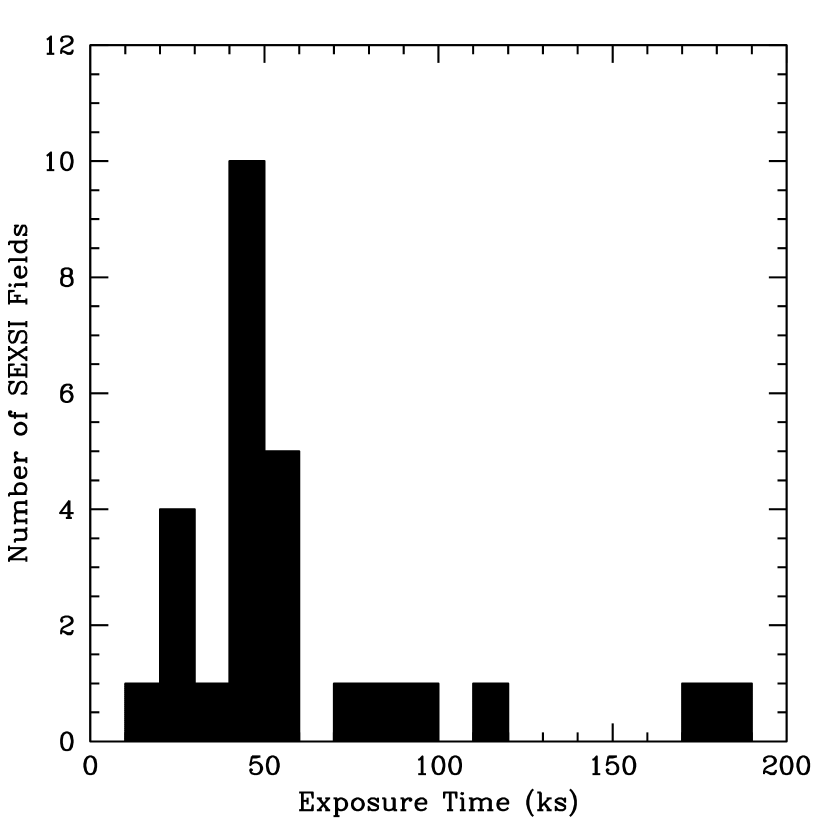
Figure 2: Histogram of exposure times for the 27 Chandra fields listed in Table 2.

Net exposure times range from 18 ks to 186 ks; a histogram of exposure times is given in Figure 2. Targets include a Galactic planetary nebula, various types of AGN, transient afterglow followup observations, NGC galaxies, and clusters of galaxies, particularly those at relatively high redshifts. For the cases in which the target is an extended X-ray source, we have taken care to exclude those sources potentially associated with the target from our $\log N-\log S$ analysis (see §3.2).

3 Data reduction and analysis

3.1 Basic X-ray reduction

The X-ray data reduction includes filtering raw event data to reject contaminating particle events, binning the event data into images with specific energy ranges, searching the images for sources, and extracting source fluxes.

For the initial processing steps, through source identification, we use standard tools supplied by the Chandra X-ray Observatory Science Center (CXC). We employ ASCA event grades 0, 2, 3, 4, 6, and we eliminate flickering pixels and events at the chip node boundaries. For each chip we bin events into soft (0.3 – 2.1 keV) and hard (2.1 – 7 keV) band images. The 2.1 keV energy boundary is chosen to coincide with the abrupt mirror reflectance change caused by the Ir M-shell edge, and the upper and lower limits optimize signal-to-noise in the images. We use wavdetect for initial source identification. In a subsequent step we test the significance of each source individually and eliminate sources with a nominal chance occurrence probability greater than $10^{-6}$.

For the remainder of the processing, we use primarily our own routines to filter the wavdetect source list to reject spurious detections, to extract source fluxes, and to correct wavdetect positions when required. In some cases, particularly at large off-axis angles where the point spread function (PSF) is relatively broad, the wavdetect positions become unreliable, with some positions differing significantly from the centroid of the photon distribution. The differences are not uniformly distributed, and most are within the expected statistical tolerance. However, in typically one or two cases per field the wavdetect position will differ unacceptably, a discrepancy that has also been noted by others (Brandt et al., 2001). We use the wavdetect positions, the standard used by most other authors, unless the PSF-normalized radial shift $\Delta r^{2}/{\rm PSF}>0.8$ arcsec, in which case we use the centroid position.

After correcting source positions, we extract photons from the image to determine source fluxes. The PSF width is a strong function of off-axis angle. To determine extraction radii, we use the encircled energy fractions tabulated by the CXC at eight off-axis angles and at five different energies. We use the 1.5 keV and 4.5 keV values for the soft and hard bands, respectively, and interpolate linearly between tabulated values in off-axis angle. For the extraction radius we use an encircled energy fraction ranging from 80 – 90%, depending on the band and off-axis angle (see Table 3). This optimizes the signal-to-noise ratio, since the optimal fraction depends on signal-to-background ratio. To determine the background level for subtraction, we identify a number of circular, source-free regions on each chip, and for each source, use the closest region to determine the background. We define a sufficient number of regions distributed over the chip to ensure that systematic background variations are small compared to statistical uncertainties.

For each wavdetect source, we use the background level in the extraction aperture to calculate a lower limit to the number of total counts for which the probability that the detection is a random fluctuation is less than $10^{-6}$. If the total extracted counts fall below this limit, we deem the candidate wavdetect source to have failed our significance criterion, and remove the source from the catalog. In on-axis chips, there are about $5\times 10^{5}$ detection cells, so we expect $\sim 0.5$ false detections per chip. Off-axis chips have 4 – 8 times fewer detection cells, as we bin them before searching. Thus, on average we expect $\leq 1$ false detection per field, depending on the number and configuration of chips read out.

To convert extracted source counts to flux, we use standard CXO software to compute energy-weighted exposure maps using a power-law spectral model with photon spectral index $\Gamma=1.5$. Using these, we convert soft band counts to a 0.5 – 2 keV flux, and hard band counts to a 2 – 10 keV flux again adopting $\Gamma=1.5$, and apply an aperture correction to account for the varying encircled energy fraction used in source extraction (see Table 3). We use the Galactic column density for each field listed in Table 2 to calculate source fluxes arriving at the Galaxy in the hard and soft bands. For an on-axis source, the conversion factor in the hard band is $S_{\rm 2-10keV}$ $\sim 3.0\times 10^{-11}\,{\rm erg}\ {\rm cm}^{-2}\ {\rm s}^{-1}$ ct^-1, although this value varies by 5-10% from field to field owing to the differences in location of the aim point relative to node and chip boundaries. We note that $\Gamma=1.5$ represents a softer spectrum than the $\Gamma=1.2-1.4$ typically used for counts to flux conversion for the deep fields; our choice was motivated by the brighter average flux of our sample.

3.2 Source deletions

In order to calculate the $\log N-\log S$ relation and to characterize the serendipitous source populations in an unbiased manner, we remove sources associated with the observation targets. In the case of point source targets such as AGN, transient afterglows, and the planetary nebula, this excision is trivial: the target object is simply excluded from the catalog. For the nearby galaxies in which the target covers a significant area of the field, we have excised all sources within an elliptical region defined where, in our optical image of the galaxy, the galactic light is $>$ 11$\sigma$ above the average background level. This led to the removal of 68 sources from the catalog. Finally, in the case of galaxy clusters, Chandra’s high angular resolution allows one to easily ‘see through’ the diffuse emission from the hot intracluster gas to the universe beyond, and it is not necessary to exclude all discrete sources for optical followup studies. Some such sources are, however, associated with the target cluster, and should not be included in our $\log N-\log S$ analysis. Thus, apart from a few sources detected in the hard band which represent the diffuse cluster emission (and have thus been removed from the catalog), we have included all discrete sources detected in the cluster fields, but have flagged all those within $\sim 1$ Mpc of the cluster centroid as potentially associated with the target. We exclude these flagged sources (and the associated effective area) from the $\log N-\log S$ analysis (a total of 190 sources). Only a small fraction of these are actually optical spectroscopically-identified cluster members.

3.3 Hardness ratio calculation

We define the hardness ratios as $(H-S)/(H+S)$, where H and S are the corrected counts in the 2 – 10 keV and 0.5 – 2 keV bands respectively. We extract the counts from our hard- (2.1–7 keV) and soft- (0.3–2.1 keV) band images using the centroids obtained by running wavdetect on the images separately (and subsequently correct the rates to the standard bands). We do this, rather than extracting counts from the soft-band image using the hard-band positions in order to minimize bias, as described below.

In a small number of cases, wavdetect failed to find a soft source both clearly present in the image and with a hard source counterpart (typically as a result of a second source very nearby). In order to correct these discrepancies, and to test for any systematic differences in soft and hard source positions, we also derived a soft flux for each source using the hard source centroid. We calculated hardness ratios using both sets of soft counts (those derived by wavdetect and those extracted using hard-source positions). Figures 3 and 4 show a comparison of the two techniques.

Using the optimal centroid position for a fixed aperture to extract source counts systematically overestimates source fluxes since the centroid selected will be influenced by positive background fluctuations to maximize the number of counts included – a form of Eddington bias; see Cowie et al. (2002). Thus, calculating hardness ratios by using soft counts extracted from a region with the hard source centroid will produce a systematic bias toward greater hardness ratios. This is illustrated in Figure 3, where we show the difference in the two methods for calculating the hardness ratio as a function of soft source flux; while only 9 sources have a difference of $>+0.05$, 48 sources have a difference of $<-0.05$. The mean bias is $-0.01$. To avoid this, we use the hardness ratios derived from the independent soft and hard source catalogs.

3.4 Calculation of the effective area function

In order to construct the hard X-ray source $\log N-\log S$ curve, we must determine the effective area of our survey as a function of source flux (shown in Figure 1). We do this by using the same algorithms we employ for the actual source extraction and flux conversion, calculated on a fine grid which samples the entire field of view. Our detailed calculation assures that, independent of the methodology used for background subtraction and source significance testing, our calculation of the effective area will be accurate. Also, since we employ significant off-axis area in the survey, calculating the response with fine sampling across the field of view is required, given the rapid PSF changes with off-axis angle and telescope vignetting.

We divide the images from each chip, with the detected sources ‘blanked out’, into a fine grid sampled at a pitch of 8 pixels. At each location, we repeat the steps associated with source detection: we determine the aperture from the off-axis angle, background from the closest circular background region, and effective area from the spectrally-weighted exposure map at that location. Using these, we determine the minimum detectable flux at that location corresponding to a spurious detection probability of $10^{-6}$. We step across the grid in this manner, so that we determine accurately the sky area as a function of minimum detectable flux even for chips where the response changes significantly over the image. This procedure results in an effective area function which optimally matches the source detection procedure and supports the construction of a $\log N-\log S$ curve free of any biases which might be introduced by the approximate techniques adopted by some other surveys.

4 The source catalog

In Table 4 we present the SEXSI source catalog of 1034 hard-band discrete serendipitous X-ray sources detected as described above. Sources are designated CXOSEXSI (our IAU-registered name) followed by standard truncated source coordinates. The source positions (equinox J2000.0) are those derived from the hard-band X-ray images; in Paper II we use optical astrometry to derive mean offsets for each X-ray image and provide improved positions (although offsets are typically less than $1^{\prime\prime}$). We include only sources detected with a chance coincidence probability of $<10^{-6}$ in the hard band. The angular distance of the source position from the telescope axis is given in column 4. Columns 5 and 6 list the background-subtracted counts for each source within the specified aperture derived from the 2.1 – 7 keV image, followed by the estimated background counts in that same aperture. Column 7 gives an estimate of the signal-to-noise ratio (SNR) of the detection. The SNR is calculated using the approximate formula for the Poisson distribution with small numbers of counts given in Gehrels (1986):

$${\rm SNR}=\frac{{\rm source~{}counts}}{1+\sqrt{0.75+{\rm source~{}counts+background~{}counts}}}~{};$$ (1)

for high-count sources Equation 1 converges to the Gaussian limit. Owing to the relatively large background regions we have employed, the background error is negligible in the SNR calculation. It should be emphasized that these values are not a measure of source significance (which is $P<10^{-6}$ in all cases) but is a measure of the uncertainty in the source flux estimates. Column 8 shows the unabsorbed hard band flux (in units of $10^{-15}\,{\rm erg}\ {\rm cm}^{-2}\ {\rm s}^{-1}$), corrected for source counts falling outside the aperture and translated to the standard 2 – 10 keV band assuming a power law photon spectral index of $\Gamma=1.5$ and a Galactic absorbing column density appropriate to the field (see Table 2). Columns 9 – 12 provide the analogous values for the soft band. We derived soft-band fluxes by employing the same procedures on the wavdetect output from the 0.3 – 2.1 keV images, and then matching sources in the two bands. The soft fluxes are presented in the 0.5 – 2 keV. There are a large number of soft sources which lack a statistically significant hard counterpart; however, as we are interested in the 2 – 10 keV source populations, these sources are not included in the Table or considered further here. We do include a catalog of the soft band only sources in the Appendix.

4.1 Comparison of methodology with previous work

As Cowie et al. (2002) have recently discussed, the details of source detection and flux extraction can have non-trivial effects on the final source catalog derived from an X-ray image, as well as on conclusions drawn from the $\log N-\log S$ relation. As a test of our methodology, we have compared our results on one of the deeper fields in our sample, CL0848+4454, with the analysis published by Stern et al. (2002b; the SPICES survey) which uses the same technique as Giacconi et al. (2002) apply to the CDF-S. The source detection algorithm, the flux estimation method, and the effective area calculations all differ from ours, so a comparison is instructive.

Stern et al. (2002b) use the SExtractor source detection algorithm (Bertin & Arnouts, 1996) applied to a version of the 0.5 – 7 keV image with a smoothed background and a signal-to-noise cut of 2.1. They measure source fluxes using a source aperture of $R_{S}=2.4~{}\times$ the PSF full-width at half-maximum, with the background derived from an annulus $R_{S}+2^{\prime\prime}$ to $R_{S}+12^{\prime\prime}$. Their simulations predict five false sources using this procedure. In contrast, we employ the wavdetect algorithm to generate a list of source candidates from the 2.1 – 7 keV image, use hand-selected, source-free background regions with larger average areas to minimize statistical uncertainties, and require each source to have a probability of chance occurrence $<10^{-6}$, yielding $<1$ false source in this field. As noted above, we also calculate a fine-scale effective area function using exactly the same significance criterion for each PSF area on the image.

Figure 5 summarizes the result of comparing the two source catalogs. Apart from three bright sources in the off-axis S-6 chip which was not analyzed by Stern et al., our catalogs are identical down to a flux threshold of $10^{-14}\,{\rm erg}\ {\rm cm}^{-2}\ {\rm s}^{-1}$. At fainter fluxes, there is a large number of SPICES sources – 33 hard band detections – which fail to appear in our catalog (see Figure 5 – upper panel). We examined the hard-band images at each of these locations. In seven cases, our wavdetect algorithm indicated source candidates were present, but each failed the $P<10^{-6}$ significance test in the hard band. In most of the other cases, no source was apparent in the hard band, although quite a number had soft-band counterparts. In some cases, fortuitous background fluctuations in the annulus surrounding the source may have accounted for the reported SPICES hard-band detection. In nearly a third of the cases, a plausible optical identification has been found, so it is clear that some of these sources are real X-ray emitters. However, in no case did our algorithm suite miss a source which would pass our specified threshold. Since our effective area function is calculated in a manner fully consistent with our threshold calculation, our $\log N-\log S$ will be unaffected by the absence of these faint, low-significance sources from our catalog.

The lower panel of Figure 5 indicates a systematic offset between the flux scale of the two catalogs of 15 – 20%, with our SEXSI fluxes being systematically higher. Most of this effect is explained by the count-to-flux conversion factors adopted in the two studies (3.24 and $2.79\times 10^{-11}\,{\rm erg}\ {\rm cm}^{-2}\ {\rm s}^{-1}$ ct^-1 respectively for SEXSI and SPICES), which in turn derives from the use of slightly different spectral index assumptions and a different generation of response function for the instrument. Individual fluxes for weaker sources have discrepancies of up to 40%, which can be accounted for by different flux extraction and background subtraction algorithms applied to low-count-rate sources.

In summary, the differences between the two analyses of this field, while producing catalogs differing at the $\sim 20\%$ level in both source existence and source flux, are well understood. In particular we are confident that the self-consistent method we have adopted for calculating the source detection threshold and the effective area function will yield an unbiased estimate of the true $\log N-\log S$  relation for hard-band X-ray sources.

5 The 2 – 10 keV $\mathbf{\log N-\log S}$ relation

The CDF-N and -S have provided good measurements of the 2 – 10 keV  $\log N-\log S$ relationship at fluxes below $\sim 10^{-14}\,{\rm erg}\ {\rm cm}^{-2}\ {\rm s}^{-1}$ . In comparison, the SEXSI sample includes 478 sources with fluxes between $10^{-12}$ and $10^{-14}\,{\rm erg}\ {\rm cm}^{-2}\ {\rm s}^{-1}$. By combining our measurements with the deep field results, we can constrain the $\log N-\log S$ over a broad range, which includes the break from Euclidean behavior.

We use the CDF-S fluxes from Giacconi et al. (2002) along with the SEXSI sample to construct the $\log N-\log S$ between $10^{-12}$ and $10^{-15}\,{\rm erg}\ {\rm cm}^{-2}\ {\rm s}^{-1}$. For the same reasons given by Cowie et al. (2002), we choose to work with the differential curve: the differential measurement provides statistically-independent bins, and comparison does not rely on the bright-end normalization, which must be taken from other instruments. To calculate the SEXSI $\log N-\log S$, we use the effective area curve (Figure 1) to correct for incompleteness at the faint end of the sample. We have not corrected for Eddington bias which is, by comparison, a small effect. We employ the CDF-S fluxes with a correction (of about 5%) to account for the different spectral index assumption ($\Gamma=1.375$ for CDF-S compared to $\Gamma=1.5$ for SEXSI). To correct for incompleteness in the CDF-S sample, we use the effective area curve provided to us by P. Tozzi. We calculate the differential counts by binning $(N(S))$, the number of sources with flux $S$, into flux ranges, $\Delta S_{i}$, then computing the average effective area, $A_{i}$ for that range, and forming the differential curve by

$$n(S)_{i}=\sum_{S_{jmin}}^{S_{jmax}}(N(S_{j}))/(\Delta S_{i}A_{i}).$$ (2)

We normalize to a unit flux of $10^{-14}\,{\rm erg}\ {\rm cm}^{-2}\ {\rm s}^{-1}$.

Figure 6 shows the differential $\log N-\log S$ curve from the combined SEXSI and CDF-S catalogs, where the indicated errors are 1$\sigma$. The normalizations between the two agree well in the region of overlap, especially considering the different source extraction techniques and methodologies for calculating the effective area function. The combined data cannot be fit with a single power law, but require a break in slope between $1-2\times 10^{-14}\,{\rm erg}\ {\rm cm}^{-2}\ {\rm s}^{-1}$. We fit the SEXSI data with a single power law at fluxes above $1.25\times 10^{-14}\,{\rm erg}\ {\rm cm}^{-2}\ {\rm s}^{-1}$, and the CDF-S data to a separate power law below this. The fits are shown as solid and dashed lines in Figure 6. The two intersect at a flux of $1.1\times 10^{-14}\,{\rm erg}\ {\rm cm}^{-2}\ {\rm s}^{-1}$. We note that the exact position of the intersection depends on where we divide the data, but for reasonable choices yielding good fits, the break always lies in the range $1-2\times 10^{-14}\,{\rm erg}\ {\rm cm}^{-2}\ {\rm s}^{-1}$ which contains the break point first predicted on the basis of a fluctuation analysis of the Einstein Deep Survey fields nearly two decades ago (Hamilton & Helfand, 1987).

The best-fit curves are parameterized by

$$n(S)=(46.8\pm 2.1)(S/10^{-14})^{-2.46\pm 0.08}$$ (3)

for $S>1.25\times 10^{-14}\,{\rm erg}\ {\rm cm}^{-2}\ {\rm s}^{-1}$, and

$$n(S)=(43.65\pm_{2.0}^{2.1})(S/10^{-14})^{-1.41\pm 0.17}$$ (4)

below $1\times 10^{-14}\,{\rm erg}\ {\rm cm}^{-2}\ {\rm s}^{-1}$. The quoted errors are $1\sigma$ formal errors on the fits. The errors on the data points are statistical errors only, and do not include an estimate of the systematic uncertainties, such as biases on approximations in correcting for incompleteness. Based on the good agreement of the overall normalization with other surveys (see below), the systematic errors do not exceed the statistical uncertainty. The faint-end slope is dependent on where we divide the fit ranges; cutting the data at $2.5\times 10^{-14}\,{\rm erg}\ {\rm cm}^{-2}\ {\rm s}^{-1}$ yields an acceptable faint-end fit, but with a steeper slope of $-1.7$.

Figure 7 shows the fractional residuals from the best-fit curves for the SEXSI survey (top panel), the CDF-S (middle), and combined Hawaii SSA22 and CDF-N sample (Cowie et al., 2002). For the Hawaii/CDF-N data, we use the binned points (provided in digital form by L. Cowie), corrected for the different spectral slope assumed for counts to flux conversion. At the faint end, the overall normalizations agree reasonably well, with the CDF-N data systematically slightly (1$\sigma$) above the mean fit to the SEXSI and CDF-S data. The faint-end slope of $-1.41\pm 0.17$ found here is marginally steeper than the best-fit values of $-1.63\pm 0.054$ found by Cowie et al. (2002) and $-1.61\pm 0.10$ found by Rosati et al. (2002). This difference is largely due to the somewhat different normalization; in addition, as noted above, the placement of the power-law break and the binning affects the best-fit slope, so this discrepancy is not significant. Above $2\times 10^{-14}\,{\rm erg}\ {\rm cm}^{-2}\ {\rm s}^{-1}$, the deep fields contain only 2 – 3 bins, and so the shape is much better constrained by the SEXSI data. Our best-fit slope at the bright end is $-2.46\pm 0.08$, consistent both with a Euclidean source distribution, and with the value of $-2.57\pm 0.22$ found for the Hawaii+CDF-N data.

6 X-ray properties of the sample

Most SEXSI sources have too few X-ray counts to warrant spectral fitting, so we rely upon hardness ratios ($HR$) to characterize the spectral slope. As discussed in §3.3, we calculate the hardness ratio for each source, listed in column 13 of Table 4, using positions determined by independently searching the hard and soft images. We assign hard-band sources that have no soft-band wavdetect counterpart at our significance level a $HR$ of 1.0. We have also determined a hardness ratio derived by extracting flux from the soft-band images at the position determined by searching the hard-band images, which we designate by $HR_{H}$. Note this does not require a significant independent detection in the soft band, so that for many sources with $HR=1$, $HR_{H}<1$ (see Figure 4). For reference, the slope of the X-ray background in this energy range, $\Gamma\sim 1.4$, corresponds to a $HR$ of $-0.22$.

Figure 8 presents the $HR$ for SEXSI’s 1034 sources as a function of hard-band flux. The top panel of Figure 9 shows these same sources in an $HR$ histogram. The lower three panels of Figure 9 show the hardness ratio histogram broken into three flux ranges. The upper right corner of each panel indicates the number of sources and average $HR$ for each subsample. The entire sample has an average $HR$ of $0.108\pm 0.006$, corresponding to $\Gamma=0.96$. The histograms clearly illustrate the trend, previously noted by the Ms surveys, for higher hardness ratios at lower fluxes.

6.1 Distribution of hardness ratios

The highest flux (second from the top) panel in Figure 9 appears to show a bimodal distribution in hardness ratio, with a peak centered around $HR\sim-0.4$ ($\Gamma\sim 1.7$), and a harder, smaller peak centered around $HR\sim 0.7$ ($\Gamma\sim-0.1$). As the flux decreases, many of the harder sources move into the $HR=1$ bin, while the center of the softer distribution shifts only slightly to the right. This motivates us to split the hardness distribution at $HR=0$, and investigate the distribution of the two sub-populations separately.

Table 5 shows the result of splitting the three flux-selected histograms at $HR=0$, where we present the average value of $HR_{H}$ for the six populations. Note we use $HR_{H}$ to minimize the skew imposed by the sudden shift of sources to $HR=1$ imposed by the requirement of separate detection in the soft image. The Table shows that the means for the two populations are relatively stable as one considers fainter fluxes, but the fraction of sources in the $HR_{H}<0$ population grows (see the last column in Table 5).

Figure 10 shows the 2 – 10 keV $\log N-\log S$ relations for the SEXSI sources split at $HR=0$. We have excluded the cluster fields from this analysis to avoid bias. For the $HR<0$ plot (top panel) we fit the data with a single power law at fluxes above $2.5\times 10^{-14}\,{\rm erg}\ {\rm cm}^{-2}\ {\rm s}^{-1}$. The best-fit curve is parameterized by

$$n(S)_{HR<0.0}=(33.9\pm_{1.5}^{1.6})(S_{\rm 2-10keV}/10^{-14})^{-2.38\pm 0.13}.$$ (5)

The population clearly turns over at $\sim 1\times 10^{-14}\,{\rm erg}\ {\rm cm}^{-2}\ {\rm s}^{-1}$. Conversely, the $HR>0.0$ population (bottom panel) shows no break. We fit the hard data with a single power law at fluxes all the way down to $2.5\times 10^{-15}\,{\rm erg}\ {\rm cm}^{-2}\ {\rm s}^{-1}$. The best-fit curve is parameterized by

$$n(S)_{HR>0.0}=(14.8\pm^{1.8}_{1.6})(S_{\rm 2-10keV}/10^{-14})^{-2.24\pm 0.05}.$$ (6)

This curve is an excellent fit all the way down to the faint end of our sample. Presumably the hard sources are on average at lower redshift and thus do not exhibit the evolutionary effects likely to be responsible for the slope break until even fainter flux levels are reached.

6.2 X-ray spectral comparison to previous work

The SEXSI catalog includes only sources independently identified in the hard band images, and so excludes those sources detected only in the soft band. Thus, we expect our average hardness ratio to be significantly larger than that reported for the deep fields, which include a large fraction of soft-only sources. Indeed, Rosati et al. (2002) analyze a stacked spectrum of the CDF-S total sample and report an average power law index of $\Gamma=1.375$ ($HR=-0.2$), much softer than our average $HR=0.108$. Even the faintest subsample, $S_{\rm 2-10keV}$ $<2\times 10^{-15}\,{\rm erg}\ {\rm cm}^{-2}\ {\rm s}^{-1}$, with an average $\Gamma=1.05$ ($HR=0.04$), appears softer than our entire sample.

To make a better comparison to the CDF-S, we eliminated the soft-band only sources from their source catalog (Giacconi et al., 2002). In addition, we translated their fluxes, which had been converted from counts using $\Gamma=1.4$, to match ours, which assumed $\Gamma=1.5$ (a correction of about 5% for the hard band). We also correct for the different spectral ranges assumed for their hard count rate measurement (2 – 7 keV for CDF-S compared to 2 – 10 keV for SEXSI). Using these converted $HR$’s with the soft-band only sources ignored, we find that the average $HR$ for the CDF-S sample is $0.14\pm 0.01$, comparable to the SEXSI $HR$ of $0.108\pm 0.006$. Since CDF-S samples the fainter section of the $\log N-\log S$, their slightly higher average $HR$ is not surprising.

To further compare the surveys, we break the CDF-S sample into three flux ranges, as we did for our sample in Figure 9. The CDF-S has no sources in the bright range ($S_{\rm 2-10keV}$ $>10^{-13}\,{\rm erg}\ {\rm cm}^{-2}\ {\rm s}^{-1}$). In the medium flux range ($10^{-13}\,{\rm erg}\ {\rm cm}^{-2}\ {\rm s}^{-1}>$ $S_{\rm 2-10keV}$ $>10^{-14}\,{\rm erg}\ {\rm cm}^{-2}\ {\rm s}^{-1}$), we calculate the CDF-S average $HR$ to be $-0.09\pm 0.01$, as compared to SEXSI’s average $HR$ of $0.008\pm 0.007$. For the low flux range ($10^{-14}\,{\rm erg}\ {\rm cm}^{-2}\ {\rm s}^{-1}>$  $S_{\rm 2-10keV}$ $>10^{-15}\,{\rm erg}\ {\rm cm}^{-2}\ {\rm s}^{-1}$), the SEXSI’s average $HR$ is $0.25\pm 0.01$ as compared to $0.13\pm 0.02$ for CDF-S.

For each of these flux ranges we find the average $HR$’s of SEXSI and CDF-S to be comparable, but slightly higher for SEXSI. This is likely explained by the different survey depths and source detection processes. As with the SPICES reduction of the CL0848+0454 field, CDF-S detects sources in full band (0.5 – 7 keV) images and then extracts fluxes from the soft and hard band images regardless of detection significance in the individual bands. For a source that is below our threshold in the soft band we will report a flux of zero, while CDF-S may detect positive flux. If we compare the CDF-S $HR$’s to our $HR_{H}$ values of $-0.014\pm 0.007$ and $0.15\pm 0.01$ for the mid- and low- flux ranges, we are consistent with the CDF-S values of $-0.09$ and $0.16$.

7 Summary

We have completed the first “large”-area ($>1$ deg²) hard X-ray source survey with the Chandra Observatory, and report here the X-ray characteristics of 1034 serendipitous sources from 27 fields detected in the 2 – 10 keV band. This work represents a sample size in the critical flux interval $1\times 10^{-13}$ to $3\times 10^{-15}\,{\rm erg}\ {\rm cm}^{-2}\ {\rm s}^{-1}$ that exceeds the sum of all previous surveys by a factor of three. We present a technique for calculating the effective area of our survey which is fully consistent with our source detection algorithm; combined with the large source sample, this allows us to derive the most accurate $\log N-\log S$ relation yet produced for hard X-ray sources at fluxes fainter than $10^{-13}\,{\rm erg}\ {\rm cm}^{-2}\ {\rm s}^{-1}$. We find that the slope of the relation is Euclidean at fluxes above $10^{-14}\,{\rm erg}\ {\rm cm}^{-2}\ {\rm s}^{-1}$. Combining the complete source sample with the CDF-S deep survey data indicates a break in the $\log N-\log S$ slope at $1.1\times 10^{-14}\,{\rm erg}\ {\rm cm}^{-2}\ {\rm s}^{-1}$. Calculation of separate $\log N-\log S$  relations for the hard and soft portions of our sample shows that it is the softer hard-band sources which are responsible for this break; sources with $HR>0.0$ show no slope change down to a flux an order of magnitude fainter, suggesting (as our spectroscopic followup and that of the deep surveys of Hornschemeier et al. (2001) and Tozzi et al. (2001) have confirmed) that the hardest sources are predominantly a lower redshift sample. Future papers in this series will describe our optical observations of this sample, providing further insight into the populations of X-ray luminous objects that comprise the X-ray background.

APPENDIX

In Table 6 we present a source catalog of 879 soft-band serendipitous X-ray sources which lack a statistically significant hard-band counterpart. These sources are excluded from the main SEXSI catalog (Table 4) since the strength of SEXSI, and thus our primary scientific interest, lies in the study of 2 – 10 keV source populations.

These soft sources, detected and analyzed as described in Section 3.1, are designated CXOSEXSI (our IAU-registered name) followed by standard truncated source coordinates. The source positions (equinox J2000.0) are those derived from the soft-band X-ray images. We include only sources detected with a chance coincidence probability of $<10^{-6}$ in the soft band. The angular distance of the source position from the telescope axis is given in column 4. Columns 5 and 6 list the background-subtracted counts for each source within the specified aperture derived from the 0.5 – 2.1 keV image, followed by the estimated background counts in that same aperture. Column 7 gives an estimate of the signal-to-noise ratio (SNR) of the detection (see Section 4 for details). Again, it should be emphasized that these values are not a measure of source significance (which is $P<10^{-6}$ in all cases) but is a measure of the uncertainty in the source flux estimates. Column 8 shows the unabsorbed soft band flux (with units of $10^{-15}\,{\rm erg}\ {\rm cm}^{-2}\ {\rm s}^{-1}$), corrected for source counts falling outside the aperture and translated to the standard 0.5 – 2 keV band assuming a power law photon spectral index of $\Gamma=1.5$ and a Galactic absorbing column density appropriate to the field (see Table 2).

This soft-band only catalog does have the target sources carefully eliminated for point sources and nearby galaxies, as described for the main SEXSI catalog in Section 3.2. This led to the removal of 86 sources from this catalog. However, the sources within $\sim 1$ Mpc of target galaxy cluster centroids are not flagged, as was done with the hard sources in Table 4. In addition, there has been no attempt to search for extended sources.

Table 1: Comparison of Sources Detected in 2 – 10 keV Hard X-Ray Surveys.

	PUBLISHED SURVEYS
log Flux Range	ASCA	SAX	SSA13	CDF-N	CDF-S	Lynx	TOTAL	SEXSI
–14.5 $-$ –15.0	0	0	8	106	92	49	255	55
–14.0 $-$ –14.5	0	0	18	56	66	45	185	400
–13.5 $-$ –14.0	0	0	6	23	21	12	62	399
–13.0 $-$ –13.5	2	17	1	5	4	4	33	145
–12.5 $-$ –13.0	51	89	0	1	0	1	142	24
–12.0 $-$ –12.5	35	61	0	0	0	0	96	9
–11.5 $-$ –12.0	5	9	0	0	0	0	14	2
–11.0 $-$ –11.5	1	1	0	0	0	0	2	0
TOTALS	94	177	33	191	183	111	789	1034

Note. — Ueda et al. (2001) have recently published a catalog of 2 – 10 keV X-ray sources from the ASCA database which contains 1343 sources. Of these, 4 have a detection significance in the 2 – 10 keV band of $\mathrel{\hbox{\hbox to0.0pt{\lower 1.89444pt\hbox{$\sim$}\hss}\kern 0.0pt\raise 1.37775pt\hbox{$>$}}}3.0\sigma$ and $1\times 10^{-14}\,{\rm erg}\ {\rm cm}^{-2}\ {\rm s}^{-1}<$ $S_{\rm 2-10keV}$ $<3\times 10^{-14}\,{\rm erg}\ {\rm cm}^{-2}\ {\rm s}^{-1}$, while 112 entries lie in the range $3\times 10^{-14}\,{\rm erg}\ {\rm cm}^{-2}\ {\rm s}^{-1}<$ $S_{\rm 2-10keV}$ $<1\times 10^{-13}\,{\rm erg}\ {\rm cm}^{-2}\ {\rm s}^{-1}$. However, the effective area covered by this survey as a function of flux and the $\log N-\log S$ curves have not been presented, so we have not included these sources in the above table.

Table 2: Chandra Observations.

Target
			RA	DEC	NH	exp.	ACIS chips
Name	Type	$z$ or $cz$	(J2000)	(J2000)	[$10^{20}$ cm-2]	[ks]
NGC 891	edge-on spiral	528 km s-1	02 22 33	+42 20 57	6.7	51	S 235-8
AWM 7	galaxy cluster	0.017	02 54 28	+41 34 47	9.2	48	I:0-367
XRF 011130	X-ray flash afterglow	$\cdots$	03 05 28	+03 49 59	9.3	30	I:0-3
NGC 1569	spiral galaxy	$-$104 km s-1	04 30 49	+64 50 54	23.8	97	S:2357
3C 123	galaxy cluster	0.218	04 37 55	+29 40 14	19.0	47	S:235-8
CL 0442+2200	galaxy cluster	1.11	04 42 26	+02 00 07	9.5	44	I:0-3
CL 0848+4454	galaxy cluster	1.27	08 48 32	+44 53 56	2.8	186	I:0-367
RX J0910	galaxy cluster	1.11	09 10 39	+54 19 57	1.9	171	I:0-36
1156+295	blazar	0.729	11 59 32	+29 14 44	1.7	49	I:0-3
NGC 4244	edge-on spiral	244 km s-1	12 17 30	+37 48 32	1.8	49	S:235-8
NGC 4631	edge-on disk galaxy	606 km s-1	12 42 07	+32 32 30	1.2	59	S:235-8
HCG 62	compact group	4200 km s-1	12 53 08	$-$09 13 27	2.9	49	S:6-8
RX J1317	galaxy cluster	0.805	13 17 12	+29 11 17	1.1	111	I:0-36
BD 1338	galaxy cluster	0.640	13 38 25	+29 31 05	1.1	38	I:0-36
RX J1350	galaxy cluster	0.804	13 50 55	+60 05 09	1.8	58	I:0-36
3C 295	galaxy cluster	0.46	14 11 20	+52 12 21	1.3	23	S:236-8
GRB 010222	GRB afterglow	1.477	14 52 12	+43 01 44	1.7	18	S:236-8
QSO 1508	quasar	4.301	15 09 58	+57 02 32	1.4	89	S:2367
MKW 3S	galaxy cluster	0.045	15 21 52	+07 42 32	2.9	57	I:0-368
MS 1621	galaxy cluster	0.4281	16 23 36	+26 33 50	3.6	30	I:0-36
GRB 000926	GRB afterglow	2.038	17 04 10	+51 47 11	2.7	32	S:236-8
RX J1716	galaxy cluster	0.81	17 16 52	+67 08 31	3.8	52	I:0-36
NGC 6543	planetary nebula	0	17 58 29	+66 38 29	4.3	46	S:5-9
XRF 011030	X-ray flash afterglow	$\cdots$	20 43 32	+77 16 43	9.5	47	S:2367
MS 2053	galaxy cluster	0.583	20 56 22	$-$04 37 44	5.0	44	I:0-36
RX J2247	galaxy cluster	0.18	22 47 29	+03 37 13	5.0	49	I:0-36
Q2345	quasar pair	2.15	23 48 20	+00 57 21	3.6	74	S:2678
TOTAL						1648	134

Table 3: Percent of PSF half-width as a function of off-axis angle used to extract hard counts (the value for soft count extraction is obtained by adding 0.06% to the hard counts % of PSF half-width value). These values optimize the signal-to-noise of each detection (see §3.1).

OAA [′]	% of PSF HW
$0-3$	$90.0$
$3-5$	$87.5$
$5-10$	$85.0$
$>10$	$80.0$

Table 4: Source Catalog.

CXOSEXSI_	RA	DEC	OAA	Hard Band				Soft Band				HR
	(J2000)	(J2000)	[′]	Cts	Bkg	SNR	Flux	Cts	Bkg	SNR	Flux
(1)	(2)	(3)	(4)	(5)	(6)	(7)	(8)	(9)	(10)	(11)	(12)	(13)
J022142.6+422654	02 21 42.67	42 26 54.1	9.49	16.30	5.70	2.83	23.10	48.50	6.50	5.73	10.30	-0.33
J022143.6+421631	02 21 43.64	42 16 31.6	8.33	98.53	4.47	8.81	74.80	244.27	3.73	14.56	29.70	-0.28
J022151.6+422319	02 21 51.68	42 23 19.3	6.17	9.13	1.87	2.06	6.55	17.67	1.33	3.25	2.02	-0.16
J022205.0+422338	02 22 05.00	42 23 38.3	4.24	13.24	0.76	2.74	8.73	0.00	0.00	0.00	0.00	1.00
J022205.1+422213	02 22 05.13	42 22 13.3	3.45	10.55	0.45	2.38	6.82	12.61	0.39	2.68	1.33	0.07
J022207.1+422918	02 22 07.11	42 29 18.8	8.93	25.10	4.90	3.84	18.90	64.86	4.14	6.94	8.46	-0.33
J022210.0+422956	02 22 10.00	42 29 56.3	9.38	22.38	5.62	3.52	17.30	127.12	4.88	10.15	16.70	-0.62
J022210.8+422016	02 22 10.85	42 20 16.7	2.17	5.52	0.48	1.53	3.63	19.42	0.58	3.50	2.17	-0.46
J022211.7+421910	02 22 11.71	42 19 10.7	2.55	10.46	0.54	2.36	6.87	10.40	0.60	2.35	1.15	0.14
J022215.0+422341	02 22 15.04	42 23 41.6	3.15	23.60	1.40	3.88	15.40	122.76	1.24	10.09	8.13	-0.40
J022215.1+422045	02 22 15.11	42 20 45.1	1.32	72.69	2.31	7.49	42.90	378.26	3.74	18.39	23.70	-0.42
J022215.5+421842	02 22 15.55	42 18 42.3	2.46	11.33	2.67	2.34	6.79	13.18	3.82	2.53	0.85	0.28
J022219.3+422052	02 22 19.32	42 20 52.2	0.54	10.89	2.11	2.31	6.38	0.00	0.00	0.00	0.00	1.00
J022224.3+422139	02 22 24.37	42 21 39.0	0.91	98.89	2.11	8.92	64.60	529.79	4.21	21.96	37.20	-0.44
J022225.2+422451	02 22 25.25	42 24 51.5	4.07	196.06	1.94	12.99	128.00	852.89	3.11	28.18	57.80	-0.34
J022226.5+422155	02 22 26.55	42 21 55.0	1.35	10.90	2.10	2.32	6.48	47.75	4.25	5.78	3.03	-0.35
J022232.5+423015	02 22 32.53	42 30 15.2	9.61	59.97	7.03	6.50	53.60	61.20	4.80	6.67	9.47	0.12
J022236.3+421730	02 22 36.37	42 17 30.8	4.23	19.39	3.61	3.30	12.00	40.32	2.68	5.30	2.64	0.01
J022236.8+422858	02 22 36.80	42 28 58.3	8.57	17.32	4.68	3.00	12.90	115.64	3.36	9.68	15.10	-0.68
J022259.1+422434	02 22 59.10	42 24 34.2	7.77	42.98	4.02	5.43	32.50	17.51	4.49	3.03	2.49	0.49
J022334.0+422212	02 23 34.05	42 22 12.2	13.34	40.98	25.02	4.47	37.50	37.78	26.22	4.18	6.21	0.15
J025325.9+413941	02 53 25.98	41 39 41.2	13.76	48.27	52.73	4.35	50.30	836.51	120.5	26.18	141.00	-0.85
J025333.7+413928	02 53 33.74	41 39 28.0	12.31	62.72	45.28	5.49	62.50	180.10	122.9	9.77	29.30	-0.35
J025340.4+413019	02 53 40.44	41 30 19.8	14.60	87.55	158.4	5.24	89.60	647.21	524.7	18.36	69.40	-0.55
J025400.3+414006	02 54 00.32	41 40 06.4	7.34	286.41	9.59	15.71	230.00	804.34	19.66	27.07	122.00	-0.41

Table 5: $HR_{H}$ averages for sources with $HR_{H}<0$ and $HR_{H}>0$ (see §6.1).

Flux Range	$HR_{H}<0.0$		$HR_{H}>0.0$
$\,{\rm erg}\ {\rm cm}^{-2}\ {\rm s}^{-1}$	$\langle HR_{H}\rangle$	# Srcs	$\langle HR_{H}\rangle$	# Srcs	% of Srcs
$10^{-12}-10^{-13}$	$-0.38\pm 0.01$	26	$0.42\pm 0.02$	9	26
$10^{-13}-10^{-14}$	$-0.31\pm 0.01$	344	$0.49\pm 0.01$	201	37
$10^{-14}-10^{-15}$	$-0.29\pm 0.02$	201	$0.50\pm 0.02$	253	56

Figure 1: Area of sky surveyed as a function of hard (2 – 10 keV) X-ray flux for several hard X-ray surveys. SEXSI (solid line) samples the parameter space between the extremely deep, small area Chandra Ms surveys in the Hubble Deep Field-North (HDF-N; Brandt et al. 2001) and the Chandra Deep Field-South (CDF-S; Giacconi et al. 2002), and the shallow, wide-area BeppoSAX High Energy Large Area Survey (HELLAS; Fiore et al. 2001 – dotted line). Deep field coverage (dashed line) corresponds to the 1 Ms depths, combining both fields. HELLAS hard X-ray fluxes have been extrapolated from their published 5 – 10 keV depths to 2 – 10 keV  by multiplying by a factor of 1.96, appropriate for the average $\alpha_{E}=0.6$ they find in their survey. The large arrow indicates the break in the $\log N-\log S$  plot (Figure 6), corresponding to the flux level which dominates the hard X-ray source counts. The SEXSI survey is better-suited to exploring this flux level than either the ultra-deep Ms Chandra surveys or the shallow BeppoSAX HELLAS survey.

Figure 3: Comparison of hardness ratio $HR\equiv(H-S)/(H+S)$ as a function of hard X-ray flux ($H$; 2 – 10 keV), with soft-band flux ($S$; 0.5 – 2 keV) measured in two ways. We exclude hard-band only sources; they are plotted separately in Figure 4. Our primary methodology (see §3.3) is to produce soft-band catalogs directly from the soft-band images using wavdetect. The matched soft-band and hard-band catalogs were then used to produce soft-band registered hardness ratios $HR_{S}$; these are the hardness ratios presented as $HR$ in Table 4 and Figures 8 and 9. Alternatively, hardness ratios were derived by extracting the soft-band flux using the aperture defined by the hard-band detection; the resultant hard-band registered hardness ratios are indicated here as $HR_{H}$. This figure shows that the difference between the techniques is typically less than a 0.1 in $HR$ for any given source, with only a very slight systematic for $HR_{H}$ producing more positive hardness ratios.

Figure 4: Hardness ratio $HR_{H}\equiv(H-S)/(H+S)$ as a function of hard X-ray flux for sources lacking a counterpart in the soft X-ray catalog. The left-hand panel collapses the scatter plot, showing the histogram of hard-band registered hardness ratios. The dashed horizontal lines indicate the photon index $\Gamma$ which different hardness ratios correspond to. In Figure 8 these sources are all plotted along the horizontal line corresponding to $HR=1$. Here we extract soft-band counts using the aperture defined by the hard-band detection; when the extracted soft-band counts are negative, the resultant hard-band registered hardness ratio $HR_{H}$ is greater than unity. Visual inspection of the soft-band images of all sources with $S_{\rm 2-10keV}$ $\geq 2.5\times 10^{-14}\,{\rm erg}\ {\rm cm}^{-2}\ {\rm s}^{-1}$ verifies the lack of soft-band detections.

Figure 5: Comparison of the SEXSI and SPICES (Stern et al., 2002b) catalogs of hard-band 2 – 10 keV sources from the 185 ks Chandra/ACIS observation of the CL0848+4454 field in Lynx. The top panel shows the fraction of sources in each catalog which are identified in the other catalog, plotted with 10 sources per histogram bin. At bright fluxes, the source catalogs are identical. At lower fluxes, SPICES includes 33 sources that SEXSI does not, likely due to the different detection algorithms and detection passbands. The bottom panel compares photometry for the 78 sources which appear in both catalogs: SEXSI hard-band fluxes are systematically $\approx 18\%$ higher (dashed horizontal line).

Figure 6: Differential $\log N-\log S$ for the SEXSI survey (circles) and Chandra Deep Field South (squares). The data are plotted in units of number deg^-2 per unit flux, where the flux has been divided by $1\times 10^{-15}\,{\rm erg}\ {\rm cm}^{-2}\ {\rm s}^{-1}$. The solid lines shows a linear fit to the SEXSI data between $1\times 10^{-12}\,{\rm erg}\ {\rm cm}^{-2}\ {\rm s}^{-1}$ and $1\times 10^{-14}\,{\rm erg}\ {\rm cm}^{-2}\ {\rm s}^{-1}$, and the dashed line shows a fit to the CDF-S data between $1\times 10^{-14}\,{\rm erg}\ {\rm cm}^{-2}\ {\rm s}^{-1}$ and $1\times 10^{-15}\,{\rm erg}\ {\rm cm}^{-2}\ {\rm s}^{-1}$. The combined curve clearly changes slope at $1-2\times 10^{-14}\,{\rm erg}\ {\rm cm}^{-2}\ {\rm s}^{-1}$. Note that the agreement of the normalization between the SEXSI and CDF-S data is good.

Figure 7: The residuals, defined as (data - fit)/data, for SEXSI, CDF-S, and Hawaii SSA22 and CDF-N. The fit is our best fit to the SEXSI data at the bright end, and the CDF-S data at the faint end.

Figure 8: Hardness ratio $HR\equiv(H-S)/(H+S)$ of SEXSI sources as a function of hard X-ray (2 – 10 keV) flux. Sources detected only in the hard X-ray band are shown at a hardness ratio of $1$, while sources detected only in the soft X-ray band are not shown. Dashed horizontal lines are power-law models with different photon indices. The 190 sources flagged as potentially being associated with Chandra cluster targets ($R<$ 1 Mpc; §3.2) are marked as dots. The remaining 844 sources are marked as small, open circles. Error bars at bottom of figure show the typical uncertainties in hardness ratio measurements at three flux levels.

Figure 9: Histogram of hardness ratio values for the SEXSI 2$-$10 keV selected sample of X-ray sources. In the top panel, the open histogram shows all 1034 sources from our survey, and the solid histogram shows the subset of 844 sources which were not flagged as being potentially associated with the Chandra cluster targets ($R<1$ Mpc). Note that when statistical uncertainties are considered, the sources in the $HR=1$ peak will partially fill in the high $HR$ end of the histogram (see Figure 4). The lower three panels show the data from the top panel split into three flux ranges. Sources undetected in the soft band are indicated in text for the bottom two panels. Typical uncertainties in hardness ratio measurements for individual sources in each flux bin are indicated as $\sigma(HR)$.

Figure 10: Differential $\log N-\log S$ for the SEXSI sources split at $HR=0$. The data are plotted in units of number deg^-2 per unit flux, where the flux has been divided by $1\times 10^{-15}\,{\rm erg}\ {\rm cm}^{-2}\ {\rm s}^{-1}$. The top panel shows the $HR<0$ sources fit from $1\times 10^{-12}$ to $2.5\times 10^{-14}\,{\rm erg}\ {\rm cm}^{-2}\ {\rm s}^{-1}$. The bottom panel shows the $HR>0$ sources fit from $1\times 10^{-12}$ to $2.5\times 10^{-15}\,{\rm erg}\ {\rm cm}^{-2}\ {\rm s}^{-1}$. The soft ($HR<0$) sources clearly turn over at $\sim$ $1\times 10^{-14}\,{\rm erg}\ {\rm cm}^{-2}\ {\rm s}^{-1}$ while the hard ($HR>0$) sources do not and are well fit by a single power law to faint fluxes.

Table 6: Soft-band Only Source Catalog.

CXOSEXSI_	RA	DEC	OAA	Soft Band
	(J2000)	(J2000)	[′]	Cts	Bkg	SNR	Flux
(1)	(2)	(3)	(4)	(5)	(6)	(7)	(8)
J022045.8+421954	02 20 45.80	42 19 54.2	17.84	387.68	449.3	12.95	37.90
J022054.2+421724	02 20 54.22	42 17 24.3	16.62	421.68	482.3	13.57	40.60
J022101.0+422042	02 21 01.08	42 20 42.4	14.99	123.61	199.3	6.51	11.20
J022108.5+422008	02 21 08.52	42 20 08.2	13.64	109.91	206.0	5.85	9.88
J022111.1+421704	02 21 11.11	42 17 04.1	13.67	98.28	199.7	5.38	8.69
J022113.3+421842	02 21 13.35	42 18 42.3	12.90	197.24	163.7	9.85	17.40
J022122.8+421725	02 21 22.84	42 17 25.1	11.49	190.08	87.92	10.74	16.10
J022128.4+421826	02 21 28.41	42 18 26.2	10.23	54.50	7.50	6.11	8.94
J022131.1+422146	02 21 31.15	42 21 46.5	9.48	1800.8	8.19	41.36	222.00
J022131.2+422144	02 21 31.24	42 21 44.0	9.46	1659.9	8.10	39.66	204.00
J022131.5+423103	02 21 31.52	42 31 03.3	13.86	45.62	28.38	4.73	6.99
J022131.5+422148	02 21 31.58	42 21 48.3	9.41	1649.00	7.92	39.53	203.00
J022131.6+422144	02 21 31.61	42 21 44.1	9.39	1574.00	7.94	38.60	194.00
J022136.1+422730	02 21 36.11	42 27 30.7	10.82	19.42	9.58	3.01	3.00
J022140.9+422050	02 21 40.95	42 20 50.2	7.62	20.86	3.14	3.49	2.48
J022142.1+421947	02 21 42.18	42 19 47.4	7.47	26.10	2.90	4.04	3.10
J022144.2+423019	02 21 44.29	42 30 19.4	11.79	25.28	13.72	3.46	3.70
J022153.5+423026	02 21 53.50	42 30 26.1	10.97	25.00	8.00	3.67	3.59
J022155.1+421804	02 21 55.13	42 18 04.3	5.72	7.90	1.10	1.92	0.91
J022155.5+421749	02 21 55.56	42 17 49.8	5.77	7.84	1.16	1.90	0.90
J022202.6+421637	02 22 02.69	42 16 37.7	5.54	14.00	1.00	2.82	1.79
J022205.9+421652	02 22 05.90	42 16 52.3	4.98	27.05	0.95	4.25	2.99
J022221.6+422348	02 22 21.60	42 23 48.3	2.98	11.96	3.04	2.41	0.82
J022225.6+423526	02 22 25.61	42 35 26.7	14.63	115.19	32.81	8.73	18.10
J022225.7+422847	02 22 25.72	42 28 47.1	7.98	16.38	2.62	3.01	2.13
J022227.1+422336	02 22 27.18	42 23 36.6	2.93	34.28	3.72	4.75	2.21
J022227.5+422108	02 22 27.59	42 21 08.9	1.04	168.54	5.46	11.85	10.80
J022229.3+422852	02 22 29.30	42 28 52.7	8.15	16.07	2.93	2.95	2.09

References

- Akiyama et al. (2000) Akiyama, M. et al. 2000, ApJ, 532, 700
- Akiyama et al. (2002) Akiyama, M., Ueda, Y., and Ohta, K. 2002, IAU Colloquium 184 ‘AGN Surveys’; astro-ph/0201495
- Baldi et al. (2002) Baldi, A., Molendi, S., Comastri, A., Fiore, F., Matt, G., and Vignali, C. 2002, ApJ, 564, 190
- Barger et al. (2001a) Barger, A. J., Cowie, L. L., Bautz, M. W., Brandt, W. N., Garmire, G. P., Hornschemeier, A. E., Ivison, R. J., and Owen, F. N. 2001a, AJ, 122, 2177
- Barger et al. (2002) Barger, A. J., Cowie, L. L., Brandt, W. N., Capak, P., Garmire, G. P., Hornschemeier, A. E., Steffen, A. T., and Wehner, E. H. 2002, AJ, 124, 1839
- Barger et al. (2001b) Barger, A. J., Cowie, L. L., Mushotzky, R. F., and Richards, E. A. 2001b, AJ, 121, 662
- Bautz et al. (1998) Bautz, M. W. et al. 1998, in Proc. SPIE Vol. 3444, p. 210-224, X-Ray Optics, Instruments, and Missions, Richard B. Hoover; Arthur B. Walker; Eds., 210–224
- Bertin & Arnouts (1996) Bertin, E. and Arnouts, S. 1996, A&AS, 117, 393
- Brandt et al. (2001) Brandt, W. N. et al. 2001, AJ, 122, 2810
- Cagnoni et al. (1998) Cagnoni, I., della Ceca, R., and Maccacaro, T. 1998, ApJ, 493, 54
- Cowie et al. (2002) Cowie, L. L., Garmire, G. P., Bautz, M. W., Barger, A. J., Brandt, W. N., and Hornschemeier, A. E. 2002, ApJ, 566, L5
- Dickey & Lockman (1990) Dickey, J. M. and Lockman, F. J. 1990, ARA&A, 28, 215
- Eckart et al. (2003) Eckart, M. E., Laird, E., Stern, D., Mao, P. H., Harrison, F. A., and Helfand, D. J. 2003, in preparation
- Gehrels (1986) Gehrels, N. 1986, ApJ, 303, 336
- Giacconi et al. (2002) Giacconi, R. et al. 2002, ApJS, 139, 369
- Giommi et al. (2000) Giommi, P., Perri, M., and Fiore, F. 2000, A&A, 362, 799
- Hamilton & Helfand (1987) Hamilton, T. T. and Helfand, D. J. 1987, ApJ, 318, 93
- Hooper & ChaMP Collaboration (2002) Hooper, E. J. and ChaMP Collaboration. 2002, BAAS, 200, #13.12
- Hornschemeier et al. (2001) Hornschemeier, A. E. et al. 2001, ApJ, 554, 742
- La Franca et al. (2002) La Franca, F. et al. 2002, ApJ, 570, 100
- Mushotzky et al. (2000) Mushotzky, R. F., Cowie, L. L., Barger, A. J., and Arnaud, K. A. 2000, Nature, 404, 459
- Rosati et al. (2002) Rosati, P. et al. 2002, ApJ, 566, 667
- Stern et al. (2002a) Stern, D. et al. 2002a, ApJ, 568, 71
- Stern et al. (2002b) —. 2002b, AJ, 123, 2223
- Tozzi et al. (2001) Tozzi, P. et al. 2001, ApJ, 562, 42
- Ueda et al. (2001) Ueda, Y., Ishisaki, Y., Takahashi, T., Makishima, K., and Ohashi, T. 2001, ApJS, 133, 1
- Weisskopf et al. (1996) Weisskopf, M. C., O’dell, S. L., and van Speybroeck, L. P. 1996, in Proc. SPIE Vol. 2805, p. 2-7, Multilayer and Grazing Incidence X-Ray/EUV Optics III, Richard B. Hoover; Arthur B. Walker; Eds., 2–7