The Dual Origin of the Terrestrial Atmosphere

Abstract

The origin of the terrestrial atmosphere is one of the most puzzling enigmas in the planetary sciences. It is suggested here that two sources contributed to its formation, fractionated nebular gases and accreted cometary volatiles. During terrestrial growth, a transient gas envelope was fractionated from nebular composition. This transient atmosphere was mixed with cometary material. The fractionation stage resulted in a high Xe/Kr ratio, with xenon being more isotopically fractionated than krypton. Comets delivered volatiles having low Xe/Kr ratios and solar isotopic compositions. The resulting atmosphere had a near-solar Xe/Kr ratio, almost unfractionated krypton delivered by comets, and fractionated xenon inherited from the fractionation episode. The dual origin therefore provides an elegant solution to the long-standing ”missing xenon” paradox. It is demonstrated that such a model could explain the isotopic and elemental abundances of Ne, Ar, Kr, and Xe in the terrestrial atmosphere.

1 Introduction

Acquisition of a stable atmosphere is a prerequisite for the emergence and expansion of life on terrestrial planets, within the solar system and beyond. The development of life is expected to modify in turn the composition of the host atmosphere (Holland 1999), providing a planetary scale biosignature (Sagan et al. 1993). Noble gases convey important clues for deciphering the origin of the major volatile elements involved in life. Indeed, they span a large range of atomic masses, are chemically inert, and have many isotopes (Ozima and Podosek 1983).

To understand the origin of the terrestrial atmosphere one must understand which processes and which sources contributed to its formation. Despite its close proximity, the origin of the terrestrial atmosphere is one of the most puzzling enigmas in the planetary sciences (Hunten 1993, Marty and Dauphas 2002). Atmospheric noble gases (Ozima and Podosek 1983) are depleted relative to solar composition (Pepin 1991, Table 1 and Fig. 1). This depletion depends in first approximation on the mass, the light gases being more depleted and isotopically fractionated than the heavy ones. Such a trend is observed in meteorites (Mazor et al. 1970, Table 1 and Fig. 1) and it seems that the terrestrial atmosphere was derived from solar composition by some form of mass fractionation. However, this simple picture cannot explain the abundance and isotopic composition of atmospheric xenon. If the simple mass fractionation model was valid, we would expect that heavy noble gases be less depleted and less fractionated than light ones. Xenon (atomic weight 131.30) should be less depleted and less fractionated than krypton (atomic weight 83.80). Actually, the opposite is observed. Xenon is depleted in the terrestrial atmosphere by a factor of $4.8\times 10^{4}$ relative to solar composition while krypton is only depleted by a factor of $3.3\times 10^{4}$. Likewise, xenon isotopes are fractionated by 38.0 $\permil/{\rm amu}$ relative to solar while krypton isotopes are only fractionated by 7.6 $\permil/{\rm amu}$. Despite being heavier, xenon is more depleted and isotopically fractionated than krypton. This is known as the ”missing xenon” paradox (Pepin 1991, Tolstikhin and O’Nions 1994).

The Earth is not the only terrestrial planet having a ”missing xenon” problem. On Mars, xenon is also more depleted and more fractionated than what is expected (Owen et al. 1977, Swindle et al. 1986, Pepin 1991). It is important to note that martian xenon was apparently derived from the solar wind component SW-Xe (Swindle and Jones 1997, Mathew et al. 1998), while terrestrial xenon was derived from a hypothetical nebular component U-Xe (Pepin and Phinney 1978, Pepin 1991, Pepin 2000). Therefore, the apparent similarity between the terrestrial and martian atmosphere should not be regarded as evidence for similarity of sources but rather as evidence for similarity of processes.

Two categories of models have been envisioned for fractionating xenon isotopes. One assumes that the Earth accreted from porous planetesimals (Ozima and Nakazawa 1980, Zahnle et al. 1990a, Ozima and Zahnle 1993). In these planetesimals, gravitational separation of adsorbed nebular gases would have resulted in mass fractionation of trapped volatiles. This model fails to explain why light and heavy noble gases in the mantle are less fractionated than their atmospheric counterpart (Honda et al. 1991, Caffee et al. 1999). It also fails to explain why xenon in the martian atmosphere is fractionated from SW-Xe while terrestrial xenon is fractionated from U-Xe (Pepin 2000) and why unfractionated solar xenon is present in the martian mantle (Mathew and Marti 2001). Finally, it cannot reproduce the observed abundance and isotopic composition of light noble gases in the terrestrial atmosphere (Ozima and Zahnle 1993). The second category of models assumes that a massive gas envelope was lost to space on Earth or planetesimals (Zahnle and Kasting 1986, Sasaki and Nakazawa 1988, Hunten et al. 1987, Zahnle et al. 1990b, Pepin 1991, 1992, 1997, Hunten 1993). In this scenario, the rapid escape of a light gas would have exerted an aerodynamic drag on heavier gases. The balance between the upward aerodynamic drag and the downward gravitational attraction resulted in a mass-dependent loss of noble gases. A massive hydrogen atmosphere could have been acquired by capture of nebular gases or could have resulted from the reduction or photodissociation of water. The appropriate energy could have been deposited in the atmosphere as extreme ultraviolet radiation from the young evolving sun or as gravitational energy released during impacts.

For explaining the missing xenon paradox, both models require that the fractionated gases be mixed with a source having low Xe/Kr ratio and unfractionated isotopic ratios. The two possible sources are the mantle and comets. The Xe/Kr ratio and xenon isotopic composition of the upper mantle are very close to those of the atmosphere (Moreira et al. 1998, Table 1 and Fig. 5) and it is unclear whether volatiles degassed from the Earth could have had the low Xe/Kr ratio and unfractionated isotopic ratios required by some models (Pepin 1991, 1992, 1997, Tolstikhin and O’Nions 1994). The noble gas composition of comets can be inferred from laboratory experiments (Laufer et al. 1987, Bar-Nun et al. 1988, Bar-Nun and Owen 1998, Notesco et al. 1999, Notesco et al. 2003, Owen et al. 1992, Owen and Bar-Nun 1995a, b, Table 1 and Fig. 1). An attractive feature revealed by experiments is that noble gases trapped in amorphous water ice exhibit a clear depletion in Xe relative to Kr (Owen et al. 1992, Bar-Nun and Owen 1998). In other words, the Xe/Kr ratio is lower than the solar ratio (note that this would not be true if noble gases were trapped in crystalline ice as clathrate hydrates, Iro et al. 2003). This important observation prompted Owen and Bar-Nun (1992) and Zahnle et al. (1990a) to suggest that the atmospheres of the terrestrial planets represented the mixture of an internal component trapped in rocks and an external component delivered by icy planetesimals. Condensation of noble gases at low temperature in the protosolar nebula is not expected to create large isotopic fractionation (Pepin 1992). Laboratory experiments seem to support the view that if any, the fractionation is small for heavy noble gases (Notesco et al. 1999). It is assumed here that the noble gas isotopic composition of comets is solar.

As discussed previously, any mass fractionation on the early Earth would have resulted in a high Xe/Kr ratio and highly fractionated ratios in the residual atmosphere. An appealing possibility is that this residual atmosphere was mixed with cometary material having a low Xe/Kr ratio and unfractionated isotopic ratios (Fig. 2). The resulting atmosphere would have a near solar Xe/Kr ratio, almost unfractionated krypton, and highly fractionated xenon (Fig. 3). This is exactly what is observed on Earth and forms the ”missing xenon” paradox. The idea that the terrestrial atmosphere has a dual origin (Dauphas 2003), being a mixture between a fractionated atmosphere and cometary material, is the basis of this work. Note that the results presented in this contribution critically depend on the experimentally observed depletion of xenon relative to krypton when trapped in amorphous water ice.

2 Outline of the Model

Ascribing a realistic environment to the fractionation episode (stage 1) is difficult. A few observations can be made that shed some light on this stage. The first observation is that, contrary to the Earth and Mars, asteroids lack the large isotopic fractionation observed for xenon (Mazor et al. 1970). This indicates that this fractionation must be closely related to the formation of terrestrial planets. Second, the mantle stable isotopic composition is distinct from, yet very close to, the atmospheric composition (Moreira et al. 1998). This suggests that active exchange occurred between the mantle and the atmosphere through degassing or recycling. Third, some radiogenic nuclides produced in the mantle are present in the atmosphere (Ozima and Podosek 1983), implying that part of the atmosphere was degassed from the mantle. Fourth, the xenon isotopic composition of the martian atmosphere is severely fractionated while that of the martian mantle is not (Mathew and Marti 2001), supporting the view that fractionation occurred at the end of planetary accretion. Fifth, martian xenon was derived from SW-Xe while terrestrial xenon was derived from U-Xe (Swindle and Jones 1997, Mathew et al. 1998, Pepin 2000). This suggests that fractionation of xenon isotopes did not occur on planetesimals or comets. The most likely scenario is blowoff of a transient atmosphere at the end of planetary growth. Because of modeling uncertainties, it is difficult to know what is the appropriate fractionation law to apply. Instead, one may use a phenomenological model such as the generalized power law (Maréchal et al. 1999) which is written,

$${\rm r}={\rm R}\times g^{i^{n}-j^{n}},$$ (1)

where r is the fractionated ratio of the nuclides $i$ and $j$, R is the initial ratio, and $g$ and $n$ are free parameters. An equivalent formulation of this law is $C^{i}_{1}/(C^{i}_{0}\,g^{i^{n}})=c$, with $c$ an arbitrary constant. It is assumed that, prior to mass fractionation, noble gases were present in solar proportions ($C^{i}_{0}=s\,C^{i}_{\odot}$, with $s$ a constant). The concentration $C_{1}^{i}$ of $i$ at the end of stage 1 can thus be related to the solar concentration $C_{\odot}$ through,

$$C^{i}_{1}=x\,C^{i}_{\odot}\,g^{i^{n}},$$ (2)

where $x$ is an arbitrary constant ($x=c\times s$). The concentration of $i$ at the end of stage 1 in the Phenomenological Model is governed by three parameters, $x$, $g$, and $n$.

After or during this fractionation episode, the Earth may have received contributions from comets (stage 2). Accretion of icy planetesimals by the Earth may have occurred in the main stage of planetary growth or might have been part of the late veneer. The late veneer refers to the material accreted by the Earth after formation of the Moon and segregation of the terrestrial core. As illustrated by the lunar cratering record, the bombardment intensity of the Earth was higher in the past than it is at present (Chyba 1990, 1991). The high and unfractionated abundances of noble metals in the terrestrial mantle (Kimura et al. 1974, Jagoutz et al. 1979) are best explained if these elements were delivered to the mantle after metal/silicate segregation. It is thus estimated that the Earth accreted $0.7-2.7\times 10^{22}$ kg of asteroids and comets after differentiation of the core (Dauphas and Marty 2002), which is known to have occurred while the short-lived nuclide ¹⁸²Hf ($t_{1/2}=9$ Ma) was still alive, within approximately 30 Ma of solar system formation (Dauphas et al. 2002a, Kleine et al. 2002, Schoenberg et al. 2002, Yin et al. 2002). The noble gas concentration of comets $C_{\circ}$ depends on the condensation temperature of ice ${\rm T}_{\circ}$. The contribution of cometary material is then,

$$C^{i}_{2}=y\,C^{i}_{\circ}({\rm T}_{\circ}),$$ (3)

where $y$ is a scaling factor defined as ${\rm M_{\circ}/M_{\oplus}}$, M_∘ being the mass of comets accreted by the Earth. The terrestrial atmosphere ($C^{i}_{a}$) is the superposition of the fractionation episode (stage 1) and the cometary accretion (stage 2),

$$C^{i}_{a}=x\,C^{i}_{\odot}\,g^{i^{n}}+y\,C^{i}_{\circ}({\rm T}_{\circ}).$$ (4)

The five parameters of the model are $x$, $g$, $n$, $y$, and T_∘. This equation can be written independently for eight nuclides. The system is overconstrained but a proper solution can be obtained by minimizing the $\chi^{2}$ merit function (Press et al. 2002).

3 Input Parameters

Of the six noble gases He, Ne, Ar, Kr, Xe, and Rn, only four can be used to infer the origin of the terrestrial atmosphere. Indeed, He is continuously lost to space and Rn isotopes are radiogenic and radioactive with short half-lives. In addition, only two isotopes of each element provide independent information on the mass fractionation. The composition of the atmosphere can therefore be described using the following parameters for each noble gas,

$$F=\left[(C^{i}/C^{j})/(C^{i}_{\odot}/C^{j}_{\odot})-1\right]/(i-j)\times 10^{3},$$ (5)

$$A=\log(C^{i}/C^{i}_{\odot}),$$ (6)

where $i$ and $j$ are two isotopes of the same element and $C_{\odot}$ denotes the solar composition (see Table 1 caption for the values of the selected ratios). The values of $F$ and $A$ for Ne, Ar, Kr, and Xe and their associated uncertainties are compiled in Table 1. Graphically, forming the atmosphere can be seen as reproducing the positions ($A$) and derivatives ($F$) of the ”noble gas curve” for neon, argon, krypton, and xenon in the abundance versus mass space.

At present, the dominant fraction of neon, argon, krypton, and xenon resides in the atmosphere (Dauphas and Marty 2002). Thus, the composition of the atmosphere (Ozima and Podosek 1983) approximates the composition of the Earth as a whole. Magmas formed at mid-ocean ridges bear important information on the composition of the shallow mantle. The ${}^{3}{\rm He}$ concentration of the mantle can be calculated (Dauphas and Marty 2002, Marty and Dauphas 2003) using the observed degassing ${\rm{}^{3}He}$ flux (1000 mol a^-1), the rate of oceanic crust formation (20 km³ a^-1), and the degree of partial melting (10 %). The mantle ³He concentration is thus estimated to be $1.5\times 10^{-15}$ mol g^-1. Note that this calculation depends on the assumption that the present ³He flux represents a reliable estimate of the time averaged flux. The abundances of the other noble gases can then be computed using elemental ratios normalized to helium (Moreira et al. 1998). Because of limited precision and large air contamination, the isotopic compositions of mantle noble gases are not yet firmly established. Within uncertainties, the isotopic compositions of argon and krypton are identical in the mantle and in the atmosphere (Marty et al. 1998, Moreira et al. 1998, Kunz 1999). The neon isotopic composition of the mantle is important as it serves as a fiducial value for deriving the composition for other noble gases (Moreira et al. 1998). Following Moreira et al. (1998) and Trieloff et al. (2000), it is assumed that the ${\rm{}^{20}Ne/^{22}Ne}$ ratio of the shallow mantle is 12.5. The actual value might be higher, up to 13.8, the solar ratio (Ballentine et al. 2001, Yokochi and Marty 2003). The xenon isotopic composition can be derived from the ${\rm{}^{128}Xe-^{129}Xe}$ correlation measured in CO₂ well gases (Caffee et al. 1999) and the inferred ${\rm{}^{129}Xe}$ excess of the mantle (Moreira et al. 1998). The mantle ${\rm{}^{128}Xe/^{130}Xe}$ ratio is thus estimated to be 0.476.

If solar composition was known with great accuracy, the abundances of every isotope could be used to constrain the curvature of the mass fractionation law. This idea was applied to xenon isotopes (Hunten et al. 1987) but it relies on the debatable assumption that U-Xe represents the initial nebular composition (Pepin and Phinney 1978, Pepin 1991, 2000). The enigmatic U-Xe is a nebular component distinct from the present solar composition. It has been first derived theoretically by Pepin and Phinney (1978) and it is used here as the initial atmospheric composition prior to fractionation. A recent search for its presence in achondrites was inconclusive (Busemann and Eugster 2002).

As stated previously, it is assumed here that the isotopic composition of noble gases in comets is that of the ambient nebula. Laboratory experiments indicate that at 30 K, the normalized abundance of neon is depleted by a factor of $5\times 10^{-3}$ relative to its initial value, and that at 50 K, it is depleted by more than a factor of $10^{-5}$ (Laufer et al. 1987). The amount of argon trapped in ice follows a power dependence on the trapping temperature (Bar-Nun et al. 1988, Bar-Nun and Owen 1998, Owen and Bar-Nun 1995a). Using experimental data (Bar-Nun and Owen 1998), the solar Ar/O ratio (Anders and Grevesse 1989), and the oxygen concentration in cometary ice (Delsemme 1988, Marty and Dauphas 2002), it is straightforward to calculate the approximate argon concentration in comets, $C_{\circ}^{36}({\rm T_{\circ}})={\rm 0.055\times 10^{-T_{\circ}/11.4}}$ mol g^-1, with T_∘ in K. Using the calculated argon concentration and the measured enrichment factors for heavy noble gases (Owen et al. 1992, Bar-Nun and Owen 1998), it is then possible to estimate the composition of comets for Kr and Xe. The enrichment factors were measured for a finite set of trapping temperatures and they have been interpolated between measurements assuming a power dependence on T_∘. The calculated composition of comets is given for a variety of trapping temperatures in Table 1. Recent trapping experiments indicate that the deposition rate affects the amount of gas trapped in amorphous water ice (Notesco et al. 2003), strengthening the need for measurements of noble gas concentrations in real comets.

4 Results

Equation (4) can be applied to two isotopes for each noble gas. There are thus eight equations in five parameters ($x$, $g$, $n$, $y$, and T_∘). The system is overconstrained and a proper solution can only be obtained by minimizing the relative distance between the simulated and the observed atmosphere. This was done using optimization algorithms implemented in $R$ (Ihaka and Gentleman 1996). The set of parameters that minimizes the $\chi^{2}$ merit function is $(x,g,n,y,{\rm T_{\circ}})=(8.158\times 10^{-15},4.701\times 10^{2},0.2614,4.407\times 10^{-7},52.36)$. The isotopic and elemental compositions of the two stages involved in atmospheric formation are displayed in Fig. 2. As illustrated, neon and xenon are inherited from the fractionation episode (stage 1) while argon and krypton are delivered by cometary material (stage 2). The resulting atmosphere (Fig. 3) has near solar Xe/Kr ratio, almost unfractionated krypton, and fractionated xenon. This scenario therefore provides an elegant solution to the long standing ”missing xenon” paradox. It explains the isotopic and elemental abundances of all noble gases in the terrestrial atmosphere. If U-Xe is assumed for the initial composition (identical to SW-Xe for light isotopes), then there is room in the modeled atmosphere for the subsequent addition of radiogenic ¹²⁹Xe and fissiogenic ^131-136Xe (Pepin 2000).

4.1 Fractionation Episode

For explaining the terrestrial atmosphere, the model requires that the mass fractionation be nonlinear. Interestingly, blowoff models with declining escape flux result in a concave downward curvature of the mass fractionation (Hunten et al. 1987, Pepin 1991). If the energy that drove the escape decreased with time, which would be the case if it was deposited as extreme ultraviolet radiation (Zahnle and Walker 1982, Pepin 1991) or impacts (Benz and Cameron 1990, Pepin 1997), then the escape flux must have decreased with time and the curvature follows. The timing of the fractionation episode is not precisely known but it can be constrained using xenon radiogenic isotopes. The nuclides ¹²⁹Xe and ^131-136Xe are the decay products of the very short-lived nuclides ¹²⁹I (t${}_{1/2}=16$ Ma) and ²⁴⁴Pu (t${}_{1/2}=80$ Ma), respectively. It is thus estimated that the Earth became retentive for xenon approximately 100 Ma after solar system formation (Podosek and Ozima 2000).

The composition of the atmosphere is, in many respects, very close to the composition of the shallow mantle (Moreira et al. 1998). For instance, there seems to be a mantle ”missing xenon” paradox (Section 3, Table 1). In addition, the atmosphere contains radiogenic nuclides that are only produced in the mantle (Ozima and Podosek 1983). Both observations suggest that part of the atmosphere was degassed from the mantle and possibly that the fractionation episode predated full accretion of the Earth. It is often assumed that hydrodynamic escape occurred after the Earth had acquired its present size (Hunten et al. 1987, Sasaki and Nakazawa 1988, Pepin 1991, 1992, 1997). Loss of a massive atmosphere could also have occurred while the Earth was still accreting material, at a time when the terrestrial core was not yet differentiated and the sun was still very active. Photodissociation or reduction of the water delivered by asteroids and comets would have formed a massive hydrogen protoatmosphere. The accretional energy released by impacts would have driven the rapid escape of this transient hydrogen atmosphere. Although appealing, such a scenario is hardly amenable to modeling (Matsui and Abe 1986, Zahnle et al. 1988). In the present section, hydrodynamic escape of a transient atmosphere is simulated using the formalism developed by Hunten et al. (1987). Detailed calculations indicate that this simple formalism captures the phenomenon in its most important features (Zahnle and Kasting 1986). The reasons why blowoff of a primordial solar atmosphere is modeled is to check whether the appropriate curvature can be obtained within a realistic environment and to test how sensitive are the parameters of the accretion stage upon the fractionation episode.

Hunten et al. (1987) developed a convenient theoretical treatment of mass fractionation during hydrodynamic escape. Advanced applications of this formalism can be found in Pepin (1991, 1992, 1997). It is assumed that the atmosphere consists of a major light constituent of mass $m$ and column density $N$, and a minor constituent $i$ of mass $m_{i}$ and column density $N_{i}$. The heavy constituent is lost to space provided that its mass is lower than a crossover mass $m_{ci}$ defined as,

$$m_{ci}=m+\frac{k{\rm T}\Phi}{b^{i}gX},$$ (7)

where $\Phi$ and $X$ are the escape flux and the mole fraction of the light constituent respectively, and $b^{i}$ is the diffusion parameter of $i$ (see Zahnle and Kasting 1986 and Pepin 1991 for numerical values). If the crossover mass is known for one nuclide $i$, it is then easily calculated for other nuclides,

$$m_{cj}=m+(m_{ci}-m)\frac{b^{i}}{b^{j}}.$$ (8)

It is assumed that $X$ remained constant near unity through time and that the escape flux decreased with time, $\Phi=\Phi_{0}\,\Psi(t)$, with $\Psi(t)$ a declining function of the time,

$$\Psi(t)=e^{-(t/\tau)^{p}},$$ (9)

where $\tau$ is the escape timescale and $p$ is a free parameter ($p=1$ corresponds to the standard exponential decay rate, $p=2$ corresponds to a scaled normal density law, and $p\rightarrow\infty$ is the step function $\Psi=1$ for $t<\tau$ and $\Psi=0$ for $\tau<t$). The escape flux of the minor constituent can be related to the escape flux of the major constituent through,

$$\Phi_{i}=\frac{N_{i}}{N}\left(\frac{m_{ci}-m_{i}}{m_{ci}-m}\right)\Phi.$$ (10)

Let us introduce $\mu_{i}=(m_{i}-m)/(m_{ci}^{0}-m)$. The rate of variation of the minor constituent $i$ can then be written as,

$$\frac{{\rm d}N_{i}}{N_{i}}=-\frac{\Phi_{0}}{N}\left[\Psi(t)-\mu_{i}\right]{\rm d}t,$$ (11)

It is now assumed that the light constituent was replenished at the same rate as it was lost to space, $N(t)=N_{0}$. For any nuclide, loss to space began at $t=0$ and continued until the time when the crossover mass was equal to the mass of the considered nuclide. This happened at $t_{if}=\Psi^{-1}(\mu_{i})$. It is then easy to integrate Eq. 11 over the proper interval to show that,

$$\ln\frac{N_{i}}{N_{i}^{0}}=\alpha\,\int_{0}^{x_{if}}\mu_{i}-e^{-x^{p}}\,{\rm d}x,$$ (12)

where $\alpha=\Phi_{0}\tau/N_{0}$, $x$ is a nondimensional integration variable ($x=t/\tau$), and $x_{if}=[-\ln(\mu_{i})]^{\frac{1}{p}}$. When $p=1$, the previous equation can be integrated analytically and takes the form (Hunten et al. 1987, Pepin 1991),

$$\ln\frac{N_{i}}{N_{i}^{0}}=\alpha\,(\mu_{i}-1-\mu_{i}\ln\mu_{i}).$$ (13)

The initial atmosphere had solar composition. The ratio $C^{i}_{0}/C^{i}_{\odot}$ was therefore independent of the nuclide and can be denoted $s$. The composition of the terrestrial atmosphere at the end of stage 1 is thus,

$$C^{i}_{1}=s\,C^{i}_{\odot}\,\frac{N_{i}}{N_{i}^{0}}.$$ (14)

The four parameters of the law are $s$, $\alpha$, $m^{0}_{cXe}$, and $p$. The second stage remains unchanged and Eq. 3 can still be applied. It was found that a large set of parameters reproduce the composition of the terrestrial atmosphere fairly well (degeneracy of the model parameters). Hunten et al. (1987) applied the very same formalism to the case of xenon alone. They limited their study to $p=1$ and concluded that $(s,\alpha,m^{0}_{cXe},p)=(0.633\times 10^{-3},13.13,345,1)$ could explain the fractionation and curvature of terrestrial xenon and that this set of parameters corresponded to a realistic environment for the early Earth. As illustrated in Table 3 (Hydrodynamic Model I), agreement between the observed and simulated atmosphere can be obtained for a set of parameters very close to that advocated by Hunten et al., $(s,\alpha,m^{0}_{cXe},p)=(0.9561\times 10^{-3},16.04,345,1)$. The appropriate curvature of the fractionation law can therefore be obtained under realistic blowoff conditions. It is worthwhile to note that such a fractionation would also explain the curvature of the xenon isotopic composition of the terrestrial atmosphere (Hunten et al. 1987) relative to its assumed progenitor, U-Xe (Pepin and Phinney 1978).

The success of the model is remarkable. There are however small discrepancies remaining between the simulated and the observed atmosphere. The most striking feature is the overabundance of neon in the simulated atmosphere (Hydrodynamic Model I, Table 3). Pepin (1997) was confronted with the same issue and suggested that the atmosphere prior to fractionation was depleted in neon. This is unlikely because the mantle He/Ne ratio is very close to solar (Honda et al. 1993, Moreira et al. 1998, Moreira and Allègre 1998) and it is difficult to find a mechanism that would have depleted neon without fractionating its abundance relative to helium. As illustrated in Table 4 (Hydrodynamic Model II), a better fit to the observed atmospheric composition can be obtained by modifying the parameterization of the escape rate $(s,\alpha,m^{0}_{cXe},p)=(2.841\times 10^{-5},12.89,140,3.980)$. The two stages invoked in the Phenomenological (Fig. 2, Table 2) and the Hydrodynamic Models (Tables 3 and 4) are very close.

To summarize, the fractionation episode can be successfully reproduced with a feasible set of parameters governing hydrodynamic escape of a transient atmosphere on the early Earth.

4.2 Cometary Accretion

How sensitive are the parameters derived for the accretion stage upon the fractionation episode? This can be investigated using the generalized power law introduced in Section 2 (Maréchal et al. 1999). Varying the power parameter of this law ($n$) allows to explore a wide variety of functional forms for the fractionation episode, including the exponential law (Dauphas 2003). It was found that the parameters of the accretionary stage were insensitive to the assumed form of the fractionation law. For instance, the parameters derived using the Phenomenological Model are $(y,{\rm T}_{\circ})=(4.407\times 10^{-7},52.36)$ and those derived using the blowoff model are $(y,{\rm T}_{\circ})=(4.409\times 10^{-7},53.26)$ or $(y,{\rm T}_{\circ})=(5.400\times 10^{-7},54.55)$, depending on the parameterization adopted for the escape rate, see Sections 2 and 4.1. The two parameters $y$ and T_∘ describe the mass of comets accreted by the Earth ($5\pm 1\times 10^{-7}$ M_⊕) and the condensation temperature of cometary ice ($50-55$ K), respectively. How do these values compare with independent estimates?

Based on the abundances of noble metals in the terrestrial mantle, it is estimated that the Earth accreted $0.7-2.7\times 10^{22}$ kg of extraterrestrial material after segregation of the core (Dauphas and Marty 2002), which is thought to have occurred within approximately $30$ Ma of solar system formation (Dauphas et al. 2002a, Kleine et al. 2002, Schoenberg et al. 2002, Yin et al. 2002). The mass of comets accreted by the Earth is calculated to be $3.0\pm 0.6\times 10^{18}$ kg (${\rm M}_{\circ}=y\,{\rm M}_{\oplus}$). If these comets were accreted after differentiation of the core, they would only represent $10^{-4}$ by mass of the late veneer. This value agrees with the estimate, based on water deuterium to protium ratios, that comets represented less than $10^{-2}$ by mass of the impacting population (Dauphas et al. 2000). At present, comets comprise a significant fraction of Earth’s impacting population, at least on the order of a few percent (Shoemaker et al. 1990). The integrated mass fraction is much lower, implying that the dynamics of asteroids and comets changed with time. Knowing the mass of comets accreted by the Earth and their composition, it is then straightforward to compute their contribution to major terrestrial volatiles. As illustrated in Table 5, the cometary contribution to the terrestrial inventory of hydrogen, carbon, and nitrogen must have been negligibly small.

If the atmosphere was derived from mantle degassing, this implies that comets were not delivered as a late veneer but were accreted during the main stage of planetary accretion. Note that cometary accretion could have been contemporaneous with fractionation of a transient atmosphere (Section 4.1).

Following different lines of evidence, Owen et al. (1992) estimated that the formation temperature of the comets that impacted the Earth must have been around 50 K, very close to the value previously derived. This is not unexpected because the ”missing xenon” paradox requires a source with a low Xe/Kr ratio, and the cometary Xe/Kr ratio is subsolar for a narrow range of trapping temperatures centered around 50 K (Owen et al. 1992, Bar-Nun and Owen 1998). Simulation of cometary trajectories in the early solar system indicates that the comets that impacted the Earth must have originated beyond the orbit of Uranus (Morbidelli et al. 2000), in a region of the nebula where the temperature was probably lower than 70 K (Yamamoto 1985). This upper-limit is consistent with the value advocated in the present contribution.

As discussed in Section 3, trapping conditions such as the deposition rate affect the amount of gas trapped in amorphous water ice (Notesco et al. 2003). The mass and temperature of comets derived here using high deposition rates (Owen et al. 1992, Bar-Nun and Owen 1998) probably represent upper-limits.

5 Origin of Water on Earth

The contribution of comets formed below 55 K to the terrestrial inventory of major volatiles must have been negligibly small (Table 5). This result agrees with the marked difference between the deuterium to protium ratio of the Earth and that of comets (Balsiger et al. 1995, Eberhardt et al. 1995, Meier et al. 1998, Bockelée-Morvan et al. 1998, Dauphas et al. 2000), and the noble gas and noble metal concentrations of the Earth (Dauphas and Marty 2002). If comets did not deliver major volatiles, how did the Earth acquire its oceans?

Water could have been delivered by a late asteroidal veneer (Dauphas et al. 2000). Some meteorite groups contain large amounts of water with the appropriate D/H ratio (Kerridge 1985). Primitive carbonaceous chondrites contain 5-10 % water. The mass of the late veneer accreted after core formation is $0.7-2.7\times 10^{22}$ kg. Hence, accretion of asteroidal material could have delivered $0.3-2.7\times 10^{21}$ kg of water. This range encompasses the mass of terrestrial oceans, $1.4\times 10^{21}$ kg. Although appealing, this idea has difficulties. First, the osmium isotopic composition of the mantle is different from that of carbonaceous chondrites (Meisel et al. 1996, 2001, Walker et al. 2001). If noble metals in the terrestrial mantle were entirely delivered by the late veneer, this would imply that carbonaceous asteroids did not impact the Earth in a late accretionary stage. Note however that the osmium isotopic composition of the mantle is reconcilable with a late carbonaceous veneer, if noble metals delivered to the mantle were mixed with the fractionated residue left over after core formation (Dauphas et al. 2002b). The recent finding in meteorites of ruthenium isotope anomalies (Chen et al. 2003), an element which was essentially all delivered to the Earth after core formation, may ultimately help to solve the question of the nature of the late veneer. A second difficulty arises with noble gases. Indeed, accretion by the Earth of water from a late carbonaceous veneer would have probably delivered too much xenon of inappropriate isotopic composition (Owen and Bar-Nun 1995a, Dauphas et al. 2000).

Owen and Bar-Nun (1995a, b) and Delsemme (1999) suggested that comets formed in the Jupiter region of the nebula delivered major volatiles. These comets would have formed at comparatively high temperature (100 K). As a consequence, they would have trapped less noble gases and would exhibit a lower D/H ratio due to exchange with protosolar hydrogen. Xenon would certainly be depleted in such comets but it seems unlikely that this depletion attained the required level for delivering water without disturbing noble gases. Morbidelli et al. (2000) modeled comet trajectories in the nascent solar system. They concluded that the contribution of cometesimals from the Jupiter zone to the terrestrial water inventory was negligible.

Unless one calls on hypothetical impactors having high H₂O/Xe ratios, late accretion by the Earth of asteroidal and cometary material does not provide a straightforward explanation to the origin of the terrestrial oceans. This may indicate that major volatiles and noble gases were decoupled at some stage of planetary formation. Hydrogen, carbon, and nitrogen form reactive compounds that can interact with the geosphere. During or at the end of planetary growth, major volatiles could have been trapped in the Earth (Matsui and Abe 1986, Morbidelli et al. 2000, Abe et al. 2000) while inert noble gases would have accumulated in a transient atmosphere. This transient atmosphere would have been lost to space as a result of impact erosion and continuous escape. Differential retention of gases during planetary growth therefore provides an elegant solution to the observed decoupling between inert and reactive gases, and explains why the terrestrial H₂O/Xe ratio is so high.

6 Mantle Noble Gases

When and where did the fractionation and accretion stages occur? Although debated, the composition of the mantle bears important information on this issue. The following discussion relies on an incomplete and uncertain description of the mantle composition and noble gas behavior. It is therefore highly speculative and should be regarded as such. The silicate Earth can be divided into two reservoirs (Allègre et al. 1986/87, Marty and Dauphas 2002). One was severely outgassed, resulting in highly radiogenic isotopic ratios. This reservoir is sampled at mid-ocean ridges and represents the shallow part of the mantle. The other was much less outgassed and is sampled by ascending mantle plumes from the deep Earth. The composition of the shallow mantle is well documented while that of the deep Earth is to a large extent unknown. The shallow mantle apparently exhibits the same ”missing xenon” paradox as the atmosphere (Section 3, Table 1). This is best explained if the atmosphere was derived in part from mantle degassing or if atmospheric volatiles were recycled in the mantle.

The view that part of the atmosphere was degassed from the mantle is supported by the presence in the atmosphere of radiogenic nuclides that are produced in the silicate Earth, ⁴He, ²¹Ne, ⁴⁰Ar, ¹²⁹Xe, and ^131-136Xe. Conversely, there is growing evidence that heavy noble gases are efficiently recycled in the mantle. Sarda et al. (1999) observed a correlation between the argon and lead isotopic compositions in mid-Atlantic ridge basalts. The most straightforward interpretation is that Ar is recycled at subduction zones (see Burnard 1999 for a different explanation). An additional piece of evidence is given by Matsumoto et al. (2001) who observed a correlation in xenoliths between the abundances of mantle derived ³He and atmospheric ³⁶Ar. If argon is indeed recycled, then this must be true for heavier noble gases, krypton and xenon.

Although very similar, the composition of the shallow mantle is not identical to the composition of the atmosphere. The most striking difference is the neon isotopic composition of the mantle (Honda et al. 1991, Trieloff et al. 2000), which is very close to solar composition. This observation, together with the fact that the Ne/He ratio of the shallow mantle is close to that of the sun (Honda et al. 1993, Moreira et al. 1998, Moreira and Allègre 1998), requires the presence of an unfractionated solar component in the Earth. The second important difference is the xenon stable isotopic composition, which is apparently less fractionated in the mantle than it is in the atmosphere (Caffee et al. 1999).

The model advocated for the formation of the terrestrial atmosphere postulates that it is derived from solar composition. If atmospheric volatiles were recycled in the mantle and mixed with solar gases trapped in the silicate Earth, this would naturally explain the fact that light noble gases share affinities with the sun while heavy noble gases share affinities with the atmosphere (Fig. 4). A complication arises with xenon, which appears to have distinct isotopic compositions in the mantle and in the atmosphere. If confirmed, this observation would require the presence of a meteoritic component in the mantle. Note that fractionation of noble gases during recycling cannot explain the xenon isotopic composition of the mantle because recycled Xe is expected to be enriched in the heavy isotopes, not depleted. If atmospheric noble gases were recycled in the mantle, the fractionation episode introduced in Section 2 could have occurred on a fully accreted planet and cometary material could have been delivered as a late veneer. It is assumed here that recycled atmospheric volatiles were mixed with solar and possibly meteoritic gases trapped in the mantle,

$$C^{i}_{m}=x\,C^{i*}_{a}+y\,C^{i}_{\odot}+z\,C^{i}_{\bullet},$$ (15)

where $C^{i*}_{a}$ represents the atmospheric composition fractionated in subduction zones (for simplicity, it is assumed here that there is no fractionation), $C^{i}_{\bullet}$ represents the meteoritic component (required for explaining the xenon isotopic composition of the mantle), and $x$, $y$, and $z$ are scaling factors. The set of parameters that minimizes the $\chi^{2}$ merit function is $(x,y,z)=(7.730\times 10^{-11},1.853\times 10^{-6},5.158\times 10^{-3})$ (Table 6). As illustrated in Fig. 5, a good agreement is obtained between the observed and the modeled mantle composition. A better fit would be obtained if noble gases were fractionated during recycling, the heavy ones being preferentially recycled relative to the light ones (Fig. 4 and 5). Such a fractionation is very likely to occur. As far as radiogenic isotopes are concerned, a formalism similar to that developed by Porcelli and Wasserburg (1995a, b) would probably apply.

Note that if recycling of noble gases does not occur, then the atmosphere could have been derived from degassing of the upper part of a stratified mantle, and the distinct solar signature of the present silicate Earth could have been acquired by subsequent homogenization of the initial layered mantle. If so, then Eq. 15 would still apply.

7 Perspectives

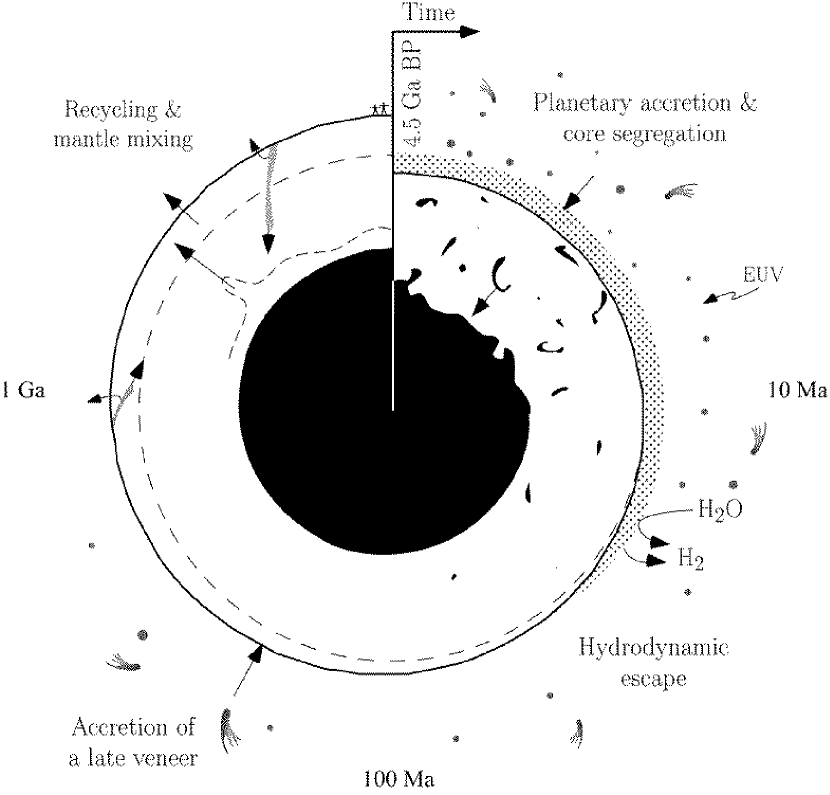
Figure 6: Cartoon illustrating the preferred scenario for the formation of the terrestial atmosphere. The silicate Earth incorporated solar and possibly meteoritic gases during its formation. Escape to space of hydrogen trapped directly from the nebula or derived from the reduction or photodissociation of water permitted the loss of heavy noble gases through hydrodynamic escape. Major volatiles which form reactive compounds with the silicate Earth were more efficiently retained by the growing planet. Within 30 Ma of the solar system formation, the core completed its formation. Extraterrestrial material accreted after that time did not equilibrate with the core and is referred to as the late veneer. Noble gases delivered by the comets accreted during this period were mixed with volatiles remaining after the escape episode. During geological times, elementally fractionated atmospheric volatiles were recycled in the mantle. The recycled atmospheric gases were mixed with gases trapped in the deep Earth during its accretion. All these successive stages may have overlapped. Timescales are indicated.

The origin of the terrestrial atmosphere is one of the most puzzling enigmas of the planetary sciences. One of the most difficult features to understand is the ”missing xenon” paradox. Being heavier, xenon should be less depleted and less fractionated than krypton. Actually, the opposite is observed. Any fractionation event on the early Earth would have resulted in high Xe/Kr and highly fractionated isotopic ratios. Interestingly, noble gases trapped in cometary ice around 50 K exhibit a clear depletion in Xe relative to Kr (Owen et al. 1992, Bar-Nun and Owen 1998). An appealing possibilty is that the terrestrial atmosphere has a dual origin, being a mixture between a fractionated atmosphere and cometary material. The resulting atmosphere would have near solar Xe/Kr, almost unfractionated krypton delivered by comets, and fractionated xenon inherited from the fractionation episode. It is demonstrated that such a model (Fig. 6) can account for the observed elemental and isotopic compositions of all noble gases in the terrestrial atmosphere. The appropriate concave downward curvature of the fractionation law can be obtained under realistic blowoff conditions for the early Earth (Hunten et al. 1987). The trapping temperature of noble gases is estimated to be lower than $55$ K, which is consistent with simulation indicating that the comets accreted by the Earth formed beyond the orbit of Uranus (Morbidelli et al. 2000). The mass of comets accreted by the Earth ($3\times 10^{18}$ kg) represents a tiny fraction ($<0.0001$) of the late veneer accreted after differentiation of the core (Dauphas and Marty 2002).

The model relies on experiments for deriving the composition of noble gases trapped in cometary ice. The processes, timescales, and location of cometary formation are still unknown. Measurement of the noble gas composition of real comets will therefore provide key information on the origin of the terrestrial atmosphere.

Table 1: Input Parameters

				${\rm Ne}$	${\rm Ar}$	${\rm Kr}$	${\rm Xe}$
Solar	$F$			0	0	0	0
	$A$			0	0	0	0
Atmosphere	$F$			$144.9$	$25.0$	$7.6$	$36.2$
	$\pm$			$3.6$	$8.9$	$1.3$	$1.6$
	$A$			$-8.21$	$-6.35$	$-4.52$	$-4.68$
	$\pm$			$0.10$	$0.10$	$0.07$	$0.08$
Mantle	$F$			47.1	25.0	7.6	31.8
	$\pm$			$8.8$	$8.9$	$1.3$	$2.4$
	$A$			-10.33	-8.76	-6.77	-6.41
	$\pm$			$0.20$	$0.20$	$0.20$	$0.20$
Comets (T∘)	$F$			0	0	0	0
	$A$	30		-0.7	1.78	1.78	1.78
		35		$<-0.7$	1.33	2.09	1.87
		40		$<-0.7$	0.90	2.19	1.81
		45		$<-0.7$	0.46	1.98	1.56
		50		$<-3.4$	0.02	1.77	1.30
		55		$<-3.4$	-0.42	1.65	1.07
		60		$<-3.4$	-0.86	1.71	1.06
		65		$<-3.4$	-1.29	1.44	1.11
		70		$<-3.4$	-1.73	1.17	1.16
Asteroids	$F$			177.5	26.8	7.4	1.0
	$A$			-6.75	-4.79	-3.19	-1.98

Note. — See Section 3 for formal definitions of $F$ and $A$. Abundances are normalized to the solar composition, ${\rm{}^{20}Ne}=8.107\times 10^{-5}$, ${\rm{}^{36}Ar}=2.153\times 10^{-6}$, ${\rm{}^{84}Kr}=6.511\times 10^{-10}$, and ${\rm{}^{130}Xe}=5.194\times 10^{-12}$ mol g^-1 (Anders and Grevesse 1989). Isotopic ratios are also normalized to the solar composition, ${\rm{}^{20}Ne/^{22}Ne=13.8\pm 0.1}$, ${\rm{}^{36}Ar/^{38}Ar=5.6\pm 0.1}$ (Wieler 1998, Pepin et al. 1999), ${\rm{}^{83}Kr/^{84}Kr=0.20291\pm 0.00026}$, and ${\rm{}^{128}Xe/^{130}Xe=0.5083\pm 0.0006}$ (Pepin 2000, Pepin et al. 1995, Wieler and Baur 1994). The trapping temperature of comets is in K. The atmospheric concentration is reported per gram of the Earth. The mantle concentration is that of the shallow mantle feeding mid-ocean ridges. Uncertainties affecting the atmospheric and mantle compositions are due to a large extent to normalization to the solar composition. Uncertainties are $2\sigma$. References: Solar- Anders and Grevesse (1989), Pepin (2000), Pepin et al. (1995, 1999), Wieler (1998), Wieler and Baur (1994). Atmosphere- Ozima and Podosek (1983). Mantle- Moreira et al. (1998), Trieloff et al. (2000), Caffee et al. (1999), Kunz (1999). Comets- Anders and Grevesse (1989), Bar-Nun et al. (1988), Bar-Nun and Owen (1998), Delsemme (1988), Marty and Dauphas (2002). Asteroids- Mazor et al. (1970).

Table 2: Phenomenological Model

			${\rm Ne}$	${\rm Ar}$	${\rm Kr}$	${\rm Xe}$
Stage 1	$F$		144.0	100.1	59.4	42.5
	$A$		-8.24	-7.27	-5.58	-4.55
Stage 2	$F$		0	0	0	0
	$A$		$<-9.9$	-6.54	-4.67	-5.19
Model	$F$		144.0	19.0	6.5	34.6
	$A$		-8.24	-6.47	-4.62	-4.46
Atmosphere	$F$		144.9	25.0	7.6	36.2
	$A$		-8.21	-6.35	-4.52	-4.68

Note. — See Section 3 for formal definitions of $F$ and $A$. Abundances and isotopic ratios are normalized to the solar composition (see Table 1 caption for details and references). Stage 1 corresponds to a fractionation episode (generalized power law). Stage 2 corresponds to the accretion by the Earth of cometary material. The model is the superposition of these two episodes (Sections 2 and 4). The parameters that minimize the distance between the modeled and the observed composition are $(x,g,n,y,{\rm T_{\circ}})=(8.158\times 10^{-15},4.701\times 10^{2},0.2614,4.407\times 10^{-7},52.36)$, see Equation 4. The results are illustrated in Figures 2 and 3.

Table 3: Hydrodynamic Model I ($p=1$)

			${\rm Ne}$	${\rm Ar}$	${\rm Kr}$	${\rm Xe}$
Stage 1	$F$		161.4	109.1	67.2	44.4
	$A$		-7.76	-7.24	-5.64	-4.82
Stage 2	$F$		0	0	0	0
	$A$		$<-9.9$	-6.62	-4.70	-5.24
Model	$F$		161.4	25.6	6.9	32.2
	$A$		-7.76	-6.53	-4.65	-4.68
Atmosphere	$F$		144.9	25.0	7.6	36.2
	$A$		-8.21	-6.35	-4.52	-4.68

Note. — See Section 3 for formal definitions of $F$ and $A$. Abundances and isotopic ratios are normalized to the solar composition (see Table 1 caption for details and references). Stage 1 corresponds to blowoff of a transient atmosphere at the end of the terrestrial accretion. Stage 2 corresponds to accretion by the Earth of cometary material. The model is the superposition of these two episodes (Section 4). Model parameters are $(s,\alpha,m^{0}_{cXe},p,y,{\rm T_{\circ}})=(0.9561\times 10^{-3},16.04,345,1,4.409\times 10^{-7},53.26)$, see Equations 3, 12, 13, and 14.

Table 4: Hydrodynamic Model II ($p\neq 1$)

			${\rm Ne}$	${\rm Ar}$	${\rm Kr}$	${\rm Xe}$
Stage 1	$F$		153.8	110.7	80.7	47.6
	$A$		-7.98	-7.48	-5.68	-4.72
Stage 2	$F$		0	0	0	0
	$A$		$<-9.9$	-6.64	-4.63	-5.20
Model	$F$		153.8	17.6	6.5	35.8
	$A$		-7.98	-6.59	-4.59	-4.59
Atmosphere	$F$		144.9	25.0	7.6	36.2
	$A$		-8.21	-6.35	-4.52	-4.68

Note. — See Section 3 for formal definitions of $F$ and $A$. Abundances and isotopic ratios are normalized to the solar composition (see Table 1 caption for details and references). Stage 1 corresponds to blowoff of a transient atmosphere at the end of the terrestrial accretion. Stage 2 corresponds to accretion by the Earth of cometary material. The model is the superposition of these two episodes (Section 4). Model parameters are $(s,\alpha,m^{0}_{cXe},p,y,{\rm T_{\circ}})=(2.841\times 10^{-5},12.89,140,3.980,5.400\times 10^{-7},54.55)$, see Equations 3, 12, and 14.

Table 5: Major Volatiles

	H	C	N
Cometary Accretion	$1.6\times 10^{20}-2.5\times 10^{20}$	$3.4\times 10^{19}-5.1\times 10^{19}$	$4.8\times 10^{18}-1.3\times 10^{19}$
Terrestrial Inventory	$1.9\times 10^{23}-1.3\times 10^{24}$	$2.1\times 10^{23}-2.1\times 10^{24}$	$4.3\times 10^{20}-7.8\times 10^{20}$

Note. — Amounts are expressed in mol. The mass of comets accreted by the Earth is $3\times 10^{18}$ kg (${\rm M_{o}}=y{\rm M}_{\oplus}$). The cometary concentrations for major volatiles are taken from Delsemme (1988) and Marty and Dauphas (2002). The terrestrial inventories refer to the bulk Earth excluding the core and are taken from Dauphas and Marty (2002).

Table 6: Mantle Model

			${\rm Ne}$	${\rm Ar}$	${\rm Kr}$	${\rm Xe}$
Stage 1	$F$		0	0	0	0
	$A$		-10.11	-10.11	-10.11	-10.11
Stage 2	$F$		177.5	26.8	7.4	1.0
	$A$		$-12.48$	-10.52	-8.92	-7.72
Stage 3	$F$		144.9	25.0	7.6	36.2
	$A$		$-10.50$	-8.64	-6.81	-6.97
Model	$F$		53.7	24.3	7.6	30.9
	$A$		-9.96	-8.62	-6.80	-6.90
Mantle	$F$		47.1	25.0	7.6	31.8
	$A$		-10.33	-8.76	-6.77	-6.41

Note. — See Section 3 for formal definitions of $F$ and $A$. Abundances and isotopic ratios are normalized to the solar composition (see Table 1 caption for details and references). Stages 1 and 2 represent the entrapment of solar and meteoritic gases in the mantle. Stage 3 corresponds to recycling of atmospheric volatiles in the silicate Earth. The model is the superposition of these three episodes. Model parameters are $(x,y,z)=(7.730\times 10^{-11},1.853\times 10^{-6},5.158\times 10^{-3})$, see Section 6, Equation 15. Note that during recycling, atmospheric volatiles would have been elementally fractionated, and stage 3 may be modified accordingly. The results are illustrated in Figures 4 and 5.

Figure 1: Normalized isotopic ($F$) and elemental ($A$) composition of the sun ($\odot$), the terrestrial atmosphere ($\oplus$), asteroids ($\bullet$), and comets formed at 55 K ($\circ$). See Section 3 and Table 1 for details and references. One would expect heavy noble gases to be less depleted and fractionated than light ones. This is not true for xenon in the terrestrial atmosphere. Despite being heavier, xenon is more depleted and more fractionated than krypton. This is known as the ”missing xenon” paradox.

Figure 2: The normalized isotopic ($F$) and elemental ($A$) compositions are reported for the two stages of atmospheric formation invoked in the Phenomenological Model (Sections 2 and 4, and Table 2). The fractionation episode was modeled using the generalized power law. The parameter set that minimizes the distance between the modeled and the observed atmosphere is $(x,g,n,y,{\rm T_{\circ}})=(8.158\times 10^{-15},4.701\times 10^{2},0.2614,4.407\times 10^{-7},52.36)$. It is assumed that at the end of Earth’s accretion, continuous loss of a transient gas envelope resulted in elemental and isotopic fractionation of the residual atmosphere (stage 1). Later or at the same time, the Earth accreted cometary material having fractionated elemental abundances but unfractionated isotopic ratios (stage 2). The resulting atmosphere would have near solar Xe/Kr ratio, almost unfractionated krypton delivered by cometary material, and fractionated xenon inherited from the fractionation episode. Such a scenario therefore provides a satisfactory solution to the ”missing xenon” paradox.

Figure 3: Isotopic ($F$) and elemental ($A$) compositions of the observed ($\oplus$) and the simulated ($\star$) atmosphere in the Phenomenological Model. The modeled atmosphere is the superposition of the two stages illustrated in Fig. 2 (Sections 2 and 4, Equation 4, and Table 2). The difference between the observed and the simulated atmosphere can be ascribed to inadequacy of the fractionation law and uncertainties regarding the compositions of comets and the nebula. Uncertainties are $2\sigma$.

Figure 4: The normalized isotopic ($F$) and elemental ($A$) compositions are reported for the three stages invoked in the Mantle Model (Section 6 and Table 6). Stages 1 and 2 represent the entrapment of solar and possibly meteoritic gases in the mantle. Stage 3 corresponds to recycling of atmospheric volatiles in the silicate Earth. The set of parameters that minimizes the relative distance between the simulated and the observed pattern is $(x,y,z)=(7.730\times 10^{-11},1.853\times 10^{-6},5.158\times 10^{-3})$. The arrows indicate the expected effect of fractionation during recycling.

Figure 5: Isotopic ($F$) and elemental ($A$) compositions of the observed ($\oplus$) and the simulated ($\star$) rare gas pattern in the Mantle Model. The modeled mantle is the superposition of the three stages illustrated in Fig. 4 (Section 6 and Table 6). The arrows indicate the direction the modeled composition would be affected if atmospheric noble gases had been fractionated during recycling, heavy elements being less depleted than light ones. Uncertainties are 2$\sigma$.