Galaxy and hot gas distributions in the z=0.52 galaxy cluster RBS380 from CHANDRA and NTT observations.

We present CHANDRA X-ray and NTT optical observations of the distant $z=0.52$ galaxy cluster RBS380 – the most distant cluster of the ROSAT Bright Source (RBS) catalogue. We find diffuse, non-spherically symmetric X-ray emission with a X-ray luminosity of $L_{X}(0.3-10$ keV$)=1.6\leavevmode\nobreak\ 10^{44}$ erg/s, which is lower than expected from the RBS. The reason is a bright AGN in the centre of the cluster contributing considerably to the X-ray flux. This AGN could not be resolved with ROSAT. In optical wavelength we identify several galaxies belonging to the cluster. The galaxy density is at least $2$ times higher than expected for such a X-ray faint cluster, which is another confirmation of the weak correlation between X-ray luminosity and optical richness. The example of the source confusion in this cluster shows how important high-resolution X-ray imaging is for cosmological research.

1 Introduction

The galaxy cluster RBS380 is part of a large optical programme to search for strong gravitationally lensed arcs in X-ray luminous clusters selected from the ROSAT Bright Survey (RBS, Schwope et al. 2000), with a predicted probability for arcs of 45%. In addition to the optical images X-ray observations are taken in order to compare masses determined with different methods and to use the X-ray morphology for lensing models. The main goal of this project is to combine X-ray and optical information, together with possible gravitational lensing information, to constrain cosmological models.

The cluster presented here – RBS380 – is after RBS797 (Schindler et al. 2001) the second cluster for which we have performed a combined optical and X-ray analysis. The X-ray source RBS380 was found in the ROSAT All-Sky Survey (RASS, Voges et al. 1996, 1999) and classified as a massive cluster of galaxies in the RBS. RBS380 is the most distant cluster of this catalogue.

We present here CHANDRA ACIS-I and NTT SUSI2 observations of the X-ray cluster RBS380 at $z=0.52$ and coordinates $\alpha=03\leavevmode\nobreak\ 01\leavevmode\nobreak\ 07.6$, $\delta=-47\leavevmode\nobreak\ 06\leavevmode\nobreak\ 35.0$ (J2000).

We find a lower X-ray luminosity than expected from the RBS. The reason is source confusion in ROSAT data – the X-ray emission of the central AGN had been mixed up with cluster emission.

The high galaxy number density in this cluster is in contrast to its low X-ray luminosity. This is another confirmation that optical luminosity is not well correlated with X-ray luminosity, see e.g. Donahue et al. (2001) or the clusters Cl0939+4713 and Cl0050-24 for extreme examples of optical richness and low X-ray luminosity (Schindler & Wambsganss 1996, 1997; Schindler et al. 1998).

Throughout this paper we use $\rm{H}_{0}=65$ km/s/Mpc, $\rm{\Omega_{M}}=0.3$ and $\rm{\Omega_{\Lambda}}=0.7$.

2 Data acquisition and reduction

2.1 X-ray data reduction

The cluster RBS380 was observed on October 17, 2000 by the CHANDRA X-ray Observatory (CXO). A single exposure of 10.3 ksec was obtained with the Advanced CCD Imaging Spectrometer (ACIS). During the observations the $2\times 2$ front-illuminated array ACIS-I was active, together with the S0 chip of the ACIS-S $1\times 6$ array, although this last one was not used for the data reduction, since the expected cluster centre was placed on the ACIS-I array. Each CCD in the ACIS-I is a $1024\times 1024$ pixel array, each pixel subtending $0^{\prime\prime}.492\times 0^{\prime\prime}.492$ on the sky, covering a total area of $16^{\prime}.9\times 16^{\prime}.9$.

The data were ground reprocessed on February 28, 2001 by the CHANDRA X-ray Center (CXC). The analysis of these reprocessed data was performed by the CIAO-2.2 suite toolkit.

As upgraded gainmaps from preprocessing were available, we used the acis_process_events tool to improve the quality of the level_2 events file. We also corrected for aspects offsets and removed bad pixels in the field. For that we used the provided bad pixel file acisf02201_000N001_bpix1.fits by the CXC. We built the lightcurve for the observation period and we searched for short high backgrounds intervals. We found none, so no data filtering was needed.

Since we are interested in the diffuse emission of the galaxy cluster, special attention has to be paid to the removal of point sources. This extra care is not needed when the count rate is high enough, since the cluster emission can be seen even without any processing. If the number of counts from diffuse cluster emission is low, any not removed point source can induce wrong estimates. In a broadband ($0.3-10$ keV) image, we applied two different procedures for the detection of sources: celldetect and wavdetect. The latter uses wavelets of differents scales and correlates them with the image; the former uses sliding square cells with the size of the instrument PSF. In general, celldetect works well with well-separated point sources, although a low threshold selection will obviously overestimate the number of point sources. On the other hand, wavdetect tends to include some diffuse emission regions as point sources. For these reasons, a scientific judgment must be applied in order to decide which regions must be identified as point sources. Using a sigma threshold of $10^{-6}$ in the wavdetect routine, we found 31 point sources, expecting a probability of wrong detections of 0.1 in the image. Using analogous criteria for the celldetect routine we found no significant differences.

The correction for telescope vignetting and variations in the spatial efficiency of the CCDs was done by means of an exposure map, using the standard procedure of the CIAO-2.2 package. The exposure map was generated for an integrated energy distribution peak. The value of the peak was slightly different depending on the included region. Selecting the whole effective area of the ACIS-I array, the peak value was 0.7 keV. If the selected area was only the region covering the central part of the cluster (a circle of radio $1^{\prime}.5$), the value of the peak was then 0.5 keV. We used these two values for the reduction and we could not see any significant change in the final result.

The background correction was done using a blank field background set acisi_C_i0123_bg_evt_230301.fits provided by the CXC. We used a blank field instead of a region from the science image, since one cannot be sure a priori whether a certain region in the field is free of galaxy cluster emission. The smoothing process for the final image was done with the csmooth CIAO tool and compared to the result using the IRAF (Image Reduction and Analysis Facility) task gauss (using a $\sigma=20$ pixels Gaussian) to be sure that no artificial features were created in the convolution process. We found no significant differences.

2.2 Optical data reduction

The galaxy cluster RBS380 was observed in optical wavelength with the New Technology Telescope (NTT) in service mode during summer 2001. The Superb Seeing Imager-2 (SUSI2) camera was used in bands V and R. The SUSI2 detector is a 2 CCDs array, $1024\times 2048$ pixels each, subtending a total area on the sky of $5^{\prime}.5\times 5^{\prime}.5$ (the pixel size in the $2\times 2$ binned mode is $0.16^{\prime\prime}/$pixel). In order to be able to avoid the gap between the two chips during the data reduction process, dithering was applied.

The data reduction was perfomed with the IRAF package. A total number of 6 images in R band and 3 in V band in very good seeing conditions ($\leq 1^{\prime\prime}$) were used in the analysis. The exposure time was 760 sec for each image. For each band, after bias subtraction, a standard flatfielding was not enough to produce good results, because the twilight flats provided by the NTT team contained some stars and the scientific images showed stronger gradients than the flats. A hyperflat (see e.g. Hainaut et al. 1998) was built to flat-correct the images. We briefly describe the hyperflat technique here.

To produce a hyperflat we processed separately the provided twilight flats and the scientific images, although the procedure will be analogous in both sets. The technique is to smooth strongly all the bias subtracted and normalized frames (with e.g a Gaussian $\sigma=100$ pixels). The result is then subtracted from the original frames, so one obtains a very flat background, but still with stars in the images. Smoothing again the result with a smaller Gaussian (e.g. $\sigma=20$ pixels) will show all the stars. One can then mark all these stars in the original frames, median average them and reject the marked values. Applying this procedure to the twilight flats set and to the scientific images set, one obtains a final twilight flat and a final night-sky flat, respectively. A linear combination of these two yields the final hyperflat.

Once the images are flatfielded, they can be co-added, resulting in a deep image of the field and free of chip gaps. Note that the whole procedure has to be done for each filter.

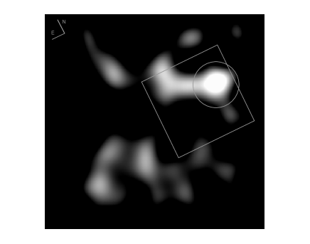
Figure 1: X-ray image of RBS380 (z=0.52) in the [0.3-10 keV] band, adaptatively smoothed with the csmooth CIAO tool and cross-check with the IRAF gauss task. The total area is $14^{\prime}\times 14^{\prime}$. The rotated square shows the region that was observed in the optical band (V and R). The circle with a radius of $1^{\prime}.5$ marks the area within which we have computed a count rate of 0.05 counts/s. Point-like X-ray sources have been removed. North and East are marked.

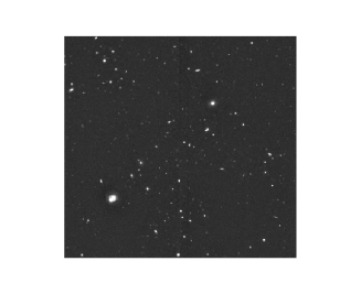
Figure 2: Optical R band image of RBS380 (z=0.52). The total area is $5^{\prime}\times 5^{\prime}$. North is up and East is left.

3 Analysis and results

3.1 X-ray results

The final X-ray image after data reduction (including point sources removal) is shown in Fig. 1. We encircle the main cluster emission within a radius of $1^{\prime}.5$ centred on the peak of the emission. The count rate obtained in that area is 0.05 counts/s. We compared this count rate to the count rate of the same region in the background fields, finding a value of 0.02 counts/s. We found that this background count rate was in fact not very sensitive to its position in the field, as expected. Using a weighted average column density $nH=2.23\leavevmode\nobreak\ 10^{20}$ cm^-2 (Dickey & Lockman 1990), a Raymond-Smith source model with $T=5$ keV and the cluster redshift $z=0.52$, the derived luminosity is $L_{X}(0.3-10{\rm{keV}})=1.6\leavevmode\nobreak\ 10^{44}$ erg/s. Using slightly lower numbers for the temperature in the source model (in the range 3-4 keV), reduces the final luminosity result in only by a few per cent. This is a relatively low X-ray luminosity for a massive cluster of galaxies. As the luminosity is so low we were particularly careful with the background subtraction and the removal of point sources.

The X-ray luminosity is lower than expected from the RBS results. The reason is an X-ray point source centred on the coordinates $\alpha=03\leavevmode\nobreak\ 01\leavevmode\nobreak\ 07.8$ and $\delta=-47\leavevmode\nobreak\ 06\leavevmode\nobreak\ 24.0$. The point source is probably an AGN which could not be resolved with ROSAT and therefore not distinguished from cluster emission. The AGN is probably the central cluster galaxy. Within a radius of $7^{\prime\prime}$ we find a count rate of 0.07 counts/s for this point source. Using a power law model with photon index 2, the same column density as for the cluster and an energy range [0.3-10 keV], the obtained flux for this AGN is $f_{X}=8.2\leavevmode\nobreak\ 10^{-13}$ erg cm² s^-1. This AGN is one of the galaxies for which the RBS optical follow-up observations (Schwope et al. 2000) yielded a redshift of 0.52 (see Fig. 7). In Table 1 we summarise the coordinates, count rates and luminosities of the AGN and the cluster.

Name	$\alpha_{2000}$	$\delta_{2000}$	Counts [cts/s]	LX [erg/s]
AGN	03 01 07.8	-47 06 24.0	0.07	1.8 1044
RBS380	03 01 07.6	-47 06 35.0	0.05	1.6 1044

Table 1: Coordinates of the AGN and the cluster. The AGN is almost at the centre of the cluster emission. We also show the count rate for the two objects (normalized for the different apertures, see text for details) and the luminosities, both in the [0.3-10 keV] band (bolometric luminosity for the cluster is given in Table 2). The contribution of the AGN is larger than the cluster luminosity. Both objects are at the same redshift of 0.52. An optical counterpart of the AGN is marked in Fig.  7.

In addition to the main cluster emission within a circle of radius $1^{\prime}.5$ described above, we found an asymmetric structure extending to both sides of this main region. If this is cluster emission, it could indicate that the cluster is not relaxed, but interacting with surrounding material or/and an infalling galaxy group. In any case we consider the inferred X-ray luminosity $L_{X}$ as an lower limit for the cluster. Due to the low number of X-ray counts we did not perform any spectral analysis.

3.2 Optical results

Both V and R images show a high number density of galaxies. The main goal is to find a way of selecting the cluster members in order to determine their number and their spatial distribution. We select cluster members through a colour-magnitude relation, applying it to all the galaxies detected both in V and R bands.

Figure 3: All the objects detected in V (upper panel) and R (lower panel) bands. A vertical stellar locus is present in both plots at the position of the seeing for each image. The magnitudes are not calibrated.

We use the SExtractor (Source-Extractor) package to build the catalogue for images V and R. First we extract all the objects detected in both images with a detection threshold of $2\sigma$ over the local sky. We show in Fig. 3 all the detected objects in both bands, representing uncalibrated magnitude vs. FWHM. In the two plots a vertical stellar locus is clearly seen at the position of the expected seeing for each image (FWHM$=1.1$ for V and FWHM$=0.75$ for R). We consider all objects to the right of these values as being galaxies. In the V band, many objects lie on the lower left side of the vertical stellar locus. We think the problem is due to the low S/N value in the final V image, built with only 3 original frames.

We select the galaxies present in both images and calibrate the magnitudes. For the calibration we use data from the SuperCOSMOS Sky Survey (SSS). We obtain from the SSS the magnitudes in R and B_J for two galaxies in our field (see both marked in Fig. 7). The calibration for our R filter is straightforward. For our V filter we use the B_J contained in the SSS. This means that our V filter is not perfectly calibrated, but the offset does not induce any difference in our results (since we are interested in the shape/slope of the colour-magnitude diagram of our galaxies, the offset induces only a vertical shift of all the objects in the plot).

Figure 4: Galaxies detected in V (upper panel) and R (lower panel) bands. The magnitudes are calibrated using the SSS archive.

In Fig. 4 we show the selected galaxies in both V and R images. Stars and deficient detections (SExtractor indicates this with different flags) are rejected. The number of galaxies is 452 in the R filter and only 64 in the V filter. This represents a 70% of the total number of objects detected in R and only a 23% of the objects detected in V.

The next step is to cross-check which galaxies detected in the V image were also detected as galaxies in the R image. We find that all the galaxies in V (64) are also present in the R catalogue.

The existence of a relation between colour and magnitude for early-type galaxies is well known (Baum 1959; Sandage & Visvanathan 1978). In Fig. 5 we show the colour-magnitude relation for the selected galaxies. Since the presence of a red sequence of early-type galaxies is an almost universal signature in clusters (Gladders et al. 1998, Gladders & Yee 2000 and references therein) and clusters at $z\approx 0.5$ tend to concentrate elliptical galaxies in their central regions (Dressler et al. 1997), we look for this sequence in our data. We select only the galaxies below 23^rd magnitude as this is our completeness limit (see Fig. 6 upper panel for completeness), and we fit the remaining galaxies by a straight line. Note that this fit is not sensitive to calibration problems, these induce only a vertical shift in the line. We used a robust statistical method based on minimizing the absolute deviation, which is expected to be less sensitive to outliers compared to standard linear regression (Press et al. 1992).

The result, presented in Fig. 6 lower panel, shows a red sequence with slope 0.06. According to the predicted slopes for formation models of galaxy clusters as a function of redshift in Gladders et al. (1998, see their Fig. 4), this slope is compatible with a galaxy cluster at $z=0.5$. This value does not strongly depend on the cosmology. This is particulary interesting because we would have derived a most likely redshift of $\approx 0.5$ from this prediction, which is in good agreement with the actual redshift of 0.52.

Figure 5: Colour-magnitude diagram for the detected galaxies both in V and R filters. Although the final number of galaxies is low due to the low number of detection in V band, a close relation can be infered at least up to a limit of 23^rd magnitude.

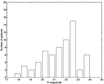
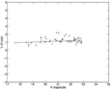
Figure 6: Upper panel: In the distribution of galaxies for the R filter we see the completeness until the 23^rd magnitude, where there is a drop in the number of galaxies detected. Lower panel: The fit shows a red sequence of the detected early-type galaxies with a slope of 0.06.

4 Comparison X-ray vs. Optical

In Fig. 7 we show the selected galaxies through the colour-magnitude relation, using the R image. We now want to compare the galaxy number density to the distribution of the X-ray emission in the same area. For the number density map, using a blank image of the same size as the optical image, we allocate pixels with value 1 in all the positions where we detected a galaxy, and then we smooth it strongly (i.e. with a 200 pixels Gaussian). We need such a large smoothing Gaussian because of the low number of galaxies finally detected. In this way we obtain the smooth distribution of the galaxies in the field.

From the X-ray image we extracted the contour lines from the squared region shown in Fig. 1 (which corresponds to the observed region in the optical). In Fig. 8 we plot the galaxy number density together with the X-ray contour lines. The main maximum peak in the number density map is shifted by $\leavevmode\nobreak\ 2$ arcmin in SE direction with respect to the X-ray maximum. Nevertheless, galaxies are present close to the asymmetric X-ray features on both sides of the main peak (in N and NE direction). These asymmetric features might indicate the existence of surrounding material interacting with the cluster, e.g. infalling galaxy groups.

The number of galaxies to the limiting magnitude is at least $2$ times higher than expected for a such faint X-ray cluster (using the number of cluster members detected in an Abell radius of $R\leq 1.5\leavevmode\nobreak\ h^{-1}$ within the centre of the cluster) but since the detection members efficiency is not complete due to the V band poor quality, this number could even be higher. This is another confirmation that number of galaxies and X-ray luminosity are not well correlated (see Table 1 for a comparison with other X-ray underluminous clusters).

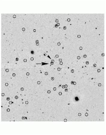
Figure 7: Optical R band image of RBS380 (z=0.52). The total area is $5^{\prime}\times 5^{\prime}$. We have inverted colours and marked the galaxies that were detected as cluster members using both R and V bands with a circle. The arrows indicate the two galaxies used for the calibration from the SSS (see text for details). The thicker arrow shows the AGN described in Sect. 3.1 and in Table 1. North is up and East is left.

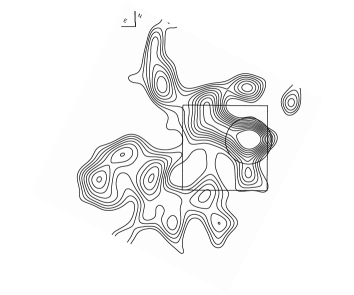
Figure 8: RBS380 galaxy number density in the R band (upper panel) and the X-rays contours for the same region (lower panel). The circle with radius $1^{\prime}.5$ is the same as in Fig. 1. The total area in both panels is $5^{\prime}\times 5^{\prime}$. North is up and East is left.

5 Conclusions

The X-ray source RBS380 was found in the RASS and identified as a cluster of galaxies in the RBS. From the RBS catalogue, the cluster was expected to be very massive due to its inferred high X-ray luminosity. Its redshift $z=0.52$ makes it the most distant galaxy cluster in that catalogue. Our interest in this object was due to its predicted probability (up to 60%) of acting as a gravitational lens. In fact these observations are part of a broader project that searches systematically for gravitational arcs in different galaxy clusters and combines this optical information with X-ray studies of the same clusters in order to constrain cosmological models and find possible correlations between X-ray and optical properties of them.

With the new CHANDRA imaging we detect a strong X-ray point source (an AGN) very close to the cluster centre, which could not be resolved with ROSAT. After subtracting the emission of this AGN, the remaining diffuse emission is almost one order of magnitude less luminous than expected: $L_{X}=1.6\leavevmode\nobreak\ 10^{44}$ erg/s. No previous investigation of the system has been carried out, so our first aim was to make sure that it is really a cluster of galaxies. The X-ray CHANDRA observation shows a non-relaxed cluster of galaxies probably interacting with surrounding material or/and another nearby cluster.

From the NTT optical observations we are able to distinguish some of the cluster members by means of the colour-magnitude relation for early-type galaxies present in the cluster, which is a well known signature for almost every cluster of galaxies. The obtained slope for this red sequence is 0.06. Using existing predicted slopes for different formation models as a function of redshift, the most likely redshift for this slope is $z\approx 0.5$, in good agreement with the measured redshift of $0.52$.

We could not detect any gravitational arc in this cluster. This is not surprising as with the low X-ray luminosity the probability for arcs is strongly reduced.

The example of this cluster shows that high-resolution X-ray imaging is crucial for cosmological research. This type of distant galaxy clusters is often used for various types of cosmological applications. Due to source confusion some clusters can have wrong luminosity measurements and hence influence the results. This effect might e.g. artificially flatten the luminosity function for distant clusters.

Name	Redshift	Luminosity [erg/s]	band
Cl0500$-$24	0.32	5.6 1044	bolometric
Cl0939$+$4713	0.41	7.9 1044	bolometric
RBS380	0.52	2  1044	bolometric

Table 2: We compare the X-ray luminosity of RBS380 with two more clusters of galaxies which are optically rich, but have relatively low X-ray luminosity. For comparison, we give the bolometric luminosity for RBS380 too.