General Relativistic Numerical Simulation on Coalescing Binary Neutron Stars and Gauge-Invariant Gravitational Wave Extraction

Abstract

We are developing 3 dimensional simulation codes for coalescing binary neutron stars. A code using the maximal slicing condition is obtained. To evaluate the gravitational radiation, we implemented a gauge-invariant wave extraction and compared the wave forms with the metric tensors at the wave zone. The energy spectrum of the waves was also evaluated to investigate the possibility that the excitation of the quasi-normal modes of the black hole, which may be formed after the merger of two stars, can be observed.

1 Introduction

We are constructing computer codes on 3D numerical relativity.[1, 2] We report here on the present status of our computer code development to study the fully general relativistic evolution of spacetimes and matter. Our main target is to study the evolution of coalescing binary neutron stars and the radiation of gravitational waves from the merger. Coalescing neutron stars or black hole binaries are the most promising sources of strong gravitational waves for interferometric detectors such as TAMA300, LIGO, VIRGO, and GEO600.[3] The first detection by these detectors may be the waves from a black hole binary because of the larger mass of the system. However the astrophysical importance of a coalescing neutron star binary is not smaller than a black hole binary. For example, in a certain model of a gamma ray bursts[4, 5], the central engine is a coalescing neutron star binary. Furthermore, a detailed analysis of the detected waves near the merger of two stars will give information on the size of a neutron star and then on the equation of state of high density matter.

Gravitational waves from coalescing binaries consist of three phases; (1) the inspiral phase, (2) the merging phase and (3) the ringing-down phase. At the inspiral phase, the separation between two stars is so large that they may be considered as point masses and the luminosity of gravitational waves is so small that the orbit of each star may be quasi-stationary. The waves from this phase is called the chirp signal and the wave form can be estimated in a post-Newtonian approximation. The coalescing binary neutron stars at the merging and the ringing-down phase cannot be considered as point masses and the general relativistic effects become large. Thus general relativistic numerical simulations are necessary to investigate the evolution of the binary at these phases and to predict the radiation of gravitational waves from the merger.

In the previous code we used the conformal slicing condition in which the metric becomes the Schwarzschild one in the outer vacuum region so that the wave extraction is easy, while for the long time integration the slicing is not stable.[1] Then we started to construct a new code using the maximal slicing condition. Disadvantages of the maximal slicing compared with the conformal slicing are 1) the extraction of gravitational waves is not straightforward, 2) more CPU hours are required since an elliptic partial differential equation should be solved for the lapse function $\alpha$. For the former, Abrahams et.al.[6] gave the gauge-invariant wave extraction technique for axially symmetric, even-parity perturbations in the Schwarzschild metric. We extend their technique to non-axially symmetric perturbations both for even- and odd-parities. As a result, we found that the gauge dependent modes in a spatial metric perturbation is so small at the vacuum exterior region that a good estimate of gravitational waves is given easily. Shibata and Uryu[7] have reported gravitational waves from the merger of binary neutron stars using a different code with different coordinate conditions so that the comparison of our results with theirs is important.

In the followings, we show recent results of our 3D general relativistic simulations of coalescence of binary neutron stars and the estimation of gravitational waves. In §2 and §3, we describe basic equations for our general relativistic code for coalescing binary neutron stars and our coordinate conditions. Numerical methods are described in §4 and we show how to extract gauge-invariant gravitational wave form in §5. In §6, numerical results of simulations of the coalescing neutron star binary are presented and §7 is devoted to the discussions.

2 Basic Equations

In order to follow the time evolution of the space-time and the matter, the Einstein equation should be reduced to a system of evolution equations. We use the (3+1)-formalism of the Einstein equation. In the (3+1)-formalism of the Einstein equation, the line element is given by

$$ds^{2}=-\alpha^{2}dt^{2}+\gamma_{ij}(dx^{i}+\beta^{i}dt)(dx^{j}+\beta^{j}dt),$$ (1)

where $\alpha$, $\beta^{i}$ and $\gamma_{ij}$ are the lapse function, the shift vector and the intrinsic metric of 3-space, respectively. The Einstein equation is decomposed to the four constraint equations and 12 evolution equations. The Hamiltonian and the momentum constraint equations are

$$R+K^{2}-K_{ij}K^{ij}=16\pi\rho_{{}_{H}},$$ (2)

and

$$D_{j}\left(K^{j}{}_{i}-\delta^{j}{}_{i}K\right)=8\pi J_{i},$$ (3)

respectively. The evolution equations are

$$\partial_{t}\gamma_{ij}=-2\alpha K_{ij}+D_{i}\beta_{j}+D_{j}\beta_{i}$$ (4)

and

$$\partial_{t}K_{ij} = \alpha\left[R_{ij}-8\pi\left\{S_{ij}+\mbox{$\frac{1}{2}$}\gamma_{ij}\left(\rho_{{}_{H}}-S^{l}{}_{l}\right)\right\}\right]-D_{i}D_{j}\alpha$$ (5)

$$+\alpha\left(KK_{ij}-2K_{il}K^{l}{}_{j}\right)+K_{li}D_{j}\beta^{l}+K_{lj}D_{i}\beta^{l}+\beta^{l}D_{l}K_{ij},$$

where $R_{ij}$ , $R=\gamma^{ij}R_{ij}$, $K_{ij}$ and $K=\gamma^{ij}K_{ij}$ are the 3-D Ricci tensor, its trace, the extrinsic curvature tensor, its trace, respectively and $D_{i}$ is the covariant derivative associated with $\gamma_{ij}$. The quantities $\rho_{{}_{H}}$, $J_{i}$ and $S_{ij}$ are the energy density, the momentum density and the stress tensor, respectively, measured by the observer moving along the line normal to the spacelike hypersurface of $t=$ constant.

In order to give initial data, the constraint equations are solved for given $\rho_{{}_{H}}$ and $J_{i}$. Here we assume that $K=0$ and $\gamma_{ij}$ is conformally flat at $t=0$ as

$$\gamma_{ij}=\phi^{4}\,\widetilde{\gamma}_{ij},$$ (6)

where $\widetilde{\gamma}_{ij}$ is the flat space metric. Defining the conformal transformation as

$$\widetilde{K}_{ij}\equiv\phi^{2}K_{ij},\quad\widetilde{K}_{i}{}^{j}\equiv\phi^{6}K_{i}{}^{j},\quad\widetilde{K}^{ij}\equiv\phi^{10}K^{ij},\quad\rho_{{}_{B}}\equiv\phi^{6}\rho_{{}_{H}},\quad\widetilde{J}_{i}\equiv\phi^{6}J_{i},$$ (7)

we can reduce Eq.(3) to

$$\widetilde{D}_{j}\widetilde{K}^{j}{}_{i}=8\pi\widetilde{J}_{i},$$ (8)

where $\widetilde{D}_{i}$ is the covariant derivative associated with $\widetilde{\gamma}_{ij}$. The traceless extrinsic curvature can be expressed as the sum of the transverse traceless part $\widetilde{K}^{\mbox{\scriptsize TT}}_{ij}$ and the longitudinal traceless part as $(LW)_{ij}$;

$$\widetilde{K}_{ij}=\widetilde{K}^{\mbox{\scriptsize TT}}_{ij}+(LW)_{ij},$$ (9)

where

$$(LW)_{ij}=\widetilde{D}_{i}W_{j}+\widetilde{D}_{j}W_{i}-\frac{2}{3}\,\widetilde{\gamma}_{ij}\widetilde{D}^{l}W_{l}.$$ (10)

Assuming $\widetilde{K}^{\mbox{\scriptsize TT}}_{ij}=0$, we have the momentum constraint equations (Eq.(8)) as

$$\widetilde{\triangle}W_{i}+\frac{1}{3}\widetilde{D}_{i}\widetilde{D}^{j}W_{j}=8\pi\widetilde{J}_{i},$$ (11)

where $\widetilde{\triangle}\equiv\widetilde{D}^{i}\widetilde{D}_{i}$.

The Hamiltonian constraint equation (Eq.(2)) becomes

$$\widetilde{\Delta}\phi=-2\pi\phi^{-1}\rho_{B}-\frac{1}{8}\phi^{-7}\widetilde{K}_{ij}\widetilde{K}^{ij}.$$ (12)

To solve the evolution of the metric tensor, we define the following variables as

$$\phi=\left(\mbox{det}(\gamma_{ij})\right)^{\frac{1}{12}},$$ (13)

$$\widetilde{\gamma}_{ij}=\phi^{-4}\gamma_{ij}\ ,$$ (14)

$$\widetilde{F}^{i}=\widetilde{\gamma}^{ij}{}_{,j}$$ (15)

$$\widehat{K}_{ij}=\phi^{-4}(K_{ij})^{\mbox{\scriptsize STF}},$$ (16)

$$K=\gamma^{ij}K_{ij}$$ (17)

where

$$\widetilde{\gamma}^{ik}\widetilde{\gamma}_{kj}=\delta^{i}{}_{j},\qquad$$ (18)

and

$$(K_{ij})^{\mbox{\scriptsize STF}}\equiv\frac{1}{2}\left(K_{ij}+K_{ji}-\frac{2}{3}\widetilde{\gamma}_{ij}\widetilde{\gamma}^{kl}K_{kl}\right).$$ (19)

The indices of $\widehat{K}_{ij}$ are lowered and raised by $\widetilde{\gamma}_{ij}$ and $\widetilde{\gamma}^{ij}$;

$$\widehat{K}^{i}{}_{j}=\widetilde{\gamma}^{ik}\widehat{K}_{kj}\ ,\qquad\widehat{K}^{ij}=\widetilde{\gamma}^{jk}\widehat{K}^{i}{}_{k}.$$ (20)

We treat $\phi$, $\widetilde{\gamma}_{ij}$, $\widetilde{F}^{i}$, $\widehat{K}_{ij}$ and $K$ as independent variables in numerical calculations, although they are not really independent. In this framework, Eq.(15) and the following equations can be treated as additional constraints,

$$\mbox{det}(\widetilde{\gamma}_{ij})=1,$$ (21)

$$\widetilde{\gamma}^{ik}\widehat{K}_{ki}=0.$$ (22)

Recently some kinds of the reformulation of the Einstein equations in numerical relativity have been proposed to obtain numerically stable codes.[8] Our formulation is the simplest one which initiated such researches of reformulations. The motivation to use the formulation is that we encountered numerical instability in development of a 3-dimensional, fully relativistic numerical simulation code and suppose that numerical errors in the second derivative of the metric tensor needed to calculate the Ricci tensor are likely to cause large errors and the instability. Then we decided to compute $\widetilde{F}^{i}$ as independent variables and calculate the Ricci tensor using $\widetilde{F}^{i}$ (see Eqs.(67)–(71)). Then we found that such modification makes the code dramatically stable. This formulation is now often cited as BSSN formulation,[9, 10] but it was first introduced by Nakamura, Oohara and Kojima,[11] and is continuously used in our code development.[2, 1, 12, 13]

From Eqs.(4) and (5), we have the evolution equations for these variables:

$$\partial_{t}\phi=-\frac{\phi}{6}\left(\alpha K-D_{l}\beta^{l}\right),$$ (23)

$$\partial_{t}\widetilde{\gamma}_{ij}=-2\left[\alpha\widehat{K}_{ij}-\phi^{-4}(D_{i}\beta_{j})^{\mbox{\scriptsize STF}}\right]\equiv\widetilde{A}_{ij},$$ (24)

$$\partial_{t}\widehat{K}_{ij} = \phi^{-4}\left\{\alpha\left[(R_{ij})^{\mbox{\scriptsize STF}}-8\pi(S_{ij})^{\mbox{\scriptsize STF}}\right]-(D_{i}D_{j}\alpha)^{\mbox{\scriptsize STF}}\right\}$$

$$+ \alpha\left(K\widehat{K}_{ij}-2\widehat{K}_{il}\widehat{K}^{l}{}_{j}\right)$$

$$+ \widehat{K}_{il}D_{j}\beta^{l}+\widehat{K}_{jl}D_{i}\beta^{l}+\phi^{-4}\beta^{l}D_{l}\left(\phi^{4}\widehat{K}_{ij}\right)-\frac{2}{3}\widehat{K}_{ij}D_{l}\beta^{l}$$

and

$$\partial_{t}K=\alpha\!\left[\widehat{K}_{ij}\widehat{K}^{ij}\!+\!\frac{1}{3}K^{2}\!+\!4\pi\!\left(\rho_{{}_{H}}\!+\!S^{i}{}_{i}\right)\right]\!-\!D^{i}D_{i}\alpha+\beta^{l}D_{l}K.$$ (26)

The quantity $\widetilde{F}^{i}$ obeys

$$\partial_{t}\widetilde{F}^{i}=-\widetilde{A}^{ij}{}_{,j},$$ (27)

since

$$\partial_{t}\widetilde{\gamma}^{ij}=-\widetilde{\gamma}^{ik}\widetilde{\gamma}^{jl}\partial_{t}\widetilde{\gamma}_{kl}=-\widetilde{\gamma}^{ik}\widetilde{\gamma}^{jl}\widetilde{A}_{kl}\equiv-\widetilde{A}^{ij}.$$ (28)

We assume that the matter is the perfect fluid, whose stress-energy is given by

$$T_{\mu\nu}=(\rho+\rho\varepsilon+p)u_{\mu}u_{\nu}+pg_{\mu\nu},$$ (29)

where $\rho$, $\varepsilon$ and $p$ are the proper mass density, the specific internal energy and the pressure, respectively, and $u_{\mu}$ is the four-velocity of the fluid. The energy density $\rho_{{}_{H}}$, the momentum density $J_{i}$ and the stress tensor $S_{ij}$ of the matter measured by the normal line observer are, respectively, given by

$$\rho_{{}_{H}}\equiv n^{\mu}n^{\nu}T_{\mu\nu},\qquad J_{i}\equiv-h_{i}{}^{\mu}n^{\nu}T_{\mu\nu},\qquad S_{ij}\equiv h_{i}{}^{\mu}h_{j}{}^{\nu}T_{\mu\nu},$$ (30)

where $n_{\mu}$ is the unit timelike four-vector normal to the spacelike hypersurface and $h_{\mu\nu}$ is the projection tensor into the hypersurface defined by

$$h_{\mu\nu}=g_{\mu\nu}+n_{\mu}n_{\nu}.$$ (31)

The relativistic hydrodynamics equations are obtained from the conservation of baryon number, $\nabla_{\mu}(\rho u^{\mu})=0$, and the energy-momentum conservation law, $\nabla_{\nu}T_{\mu}{}^{\nu}{}=0$. In order to obtain equations similar to the Newtonian hydrodynamics equations, we define $\rho_{{}_{N}}$ and $u_{i}^{N}$ by

$$\rho_{{}_{N}}\equiv\sqrt{\gamma}\alpha u^{0}\rho,\qquad u_{i}^{N}=\frac{J_{i}}{\alpha u^{0}\rho},$$ (32)

respectively, where $\gamma=\mbox{det}(\gamma_{ij})$. Then the equation for the conservation of baryon number takes the form

$$\partial_{t}\rho_{{}_{N}}+\partial_{l}\left(\rho_{{}_{N}}V^{l}\right)=0,$$ (33)

where

$$V^{l}=\frac{u^{l}}{u^{0}}=\frac{\alpha J^{l}}{p+\rho_{{}_{H}}}-\beta^{l}.$$ (34)

The equation for the momentum conservation is

$$\partial_{t}(\rho_{{}_{N}}u_{i}^{N})+\partial_{l}\left(\rho_{{}_{N}}u_{i}^{N}V^{l}\right) = -\sqrt{\gamma}\alpha\partial_{i}p-\sqrt{\gamma}(p+\rho_{{}_{H}})\partial_{i}\alpha$$ (35)

$$+\frac{\sqrt{\gamma}\alpha J^{k}J^{l}}{2(p+\rho_{{}_{H}})}\partial_{i}\gamma_{kl}+\sqrt{\gamma}J_{l}\partial_{i}\beta^{l}.$$

The equation for the internal energy conservation becomes

$$\partial_{t}(\rho_{{}_{N}}\varepsilon)+\partial_{l}\left(\rho_{{}_{N}}\varepsilon V^{l}\right)=-p\partial_{\nu}\left(\sqrt{\gamma}\alpha u^{\nu}\right).$$ (36)

To complete the hydrodynamics equations, we need an equation of state,

$$p=p(\varepsilon,\rho).$$ (37)

The right-hand side of Eq.(36) includes the time derivative. For a polytropic equation of state, $p=(\Gamma-1)\rho\varepsilon$, however, the equation reduces to

$$\partial_{t}(\rho_{{}_{N}}\varepsilon_{{}_{N}})+\partial_{l}\left(\rho_{{}_{N}}\varepsilon_{{}_{N}}V^{l}\right)=-p_{{}_{N}}\partial_{l}V^{l},$$ (38)

where

$$\varepsilon_{{}_{N}} = \left(\sqrt{\gamma}\alpha u^{0}\right)^{\Gamma-1}\,\varepsilon,$$ (39)

$$p_{{}_{N}} = (\Gamma-1)\rho_{{}_{N}}\varepsilon_{{}_{N}}=\left(\sqrt{\gamma}\alpha u^{0}\right)^{\Gamma}p.$$ (40)

3 Coordinate conditions

The choice of the shift vector $\beta^{i}$ and the lapse function $\alpha$ is important because the stability of the code largely depends on them and because it is intimately related to the extraction of physically relevant information, including gravitational radiation, in numerical relativity. Since the right-hand side of Eq.(24), $\widetilde{A}_{ij}$ is trace-free, the determinant of $\widetilde{\gamma}_{ij}$ is preserved in time and the condition

$$D_{j}\widetilde{A}^{ij}=0$$ (41)

produces the minimal distortion shift vector. This is a good choice of the spatial coordinate, but it is too complicated to be solved numerically. Instead we replace the covariant derivative in Eq. (3.1) by the partial derivative as

$$\partial_{j}\widetilde{A}^{ij}=0.$$ (42)

In this condition, we can simply set

$$\widetilde{F}^{i}=0,$$ (43)

since Eq.(27) becomes $\partial_{t}\widetilde{F}^{i}=0$ and $\widetilde{F}^{i}(t=0)=0$.

From Eqs.(24), (28) and (43), Eq.(42) is reduced to

$$\partial_{j}\widetilde{A}^{ij}=-2\partial_{j}\left(\alpha\widehat{K}^{ij}\right)+\widetilde{\gamma}^{jk}\partial_{j}\partial_{k}\beta^{i}+\frac{1}{3}\widetilde{\gamma}^{ij}\partial_{j}\partial_{k}\beta^{k}=0,$$ (44)

which yields an elliptic equation for the shift vector $\beta^{i}$:

$$\nabla^{2}\beta^{i}+\frac{1}{3}\partial_{i}\partial_{l}\beta^{l}=2\partial_{j}\left(\alpha\widehat{K}^{ij}\right)-h^{jk}\partial_{j}\partial_{k}\beta^{i}-\frac{1}{3}h^{ij}\partial_{j}\partial_{k}\beta^{k},$$ (45)

where

$$h_{ij}=\widetilde{\gamma}_{ij}-\delta_{ij}\quad\mbox{and}\quad h^{ij}=\widetilde{\gamma}^{ij}-\delta^{ij}$$ (46)

We call this condition as the pseudo-minimal distortion condition.

As for the slicing condition, we choose the maximal slicing, $K=0$. From Eq.(26), we have an elliptic equation for the lapse function $\alpha$:

$$D^{m}D_{m}\alpha=\alpha\left(\widehat{K}_{ij}\widehat{K}^{ij}+4\pi\left(\rho_{{}_{H}}+S\right)\right).$$ (47)

4 Numerical Methods

As for the spatial coordinates in numerical calculations, we use a Cartesian coordinate system $(x,y,z)$. To obtain initial data, we should solve elliptic partial differential equations of Eqs.(11) and (12). The coupled elliptic equations (11) can be reduced to four decoupled Poisson equations:

$$\triangle\chi=6\pi\partial_{i}\widetilde{J}_{i},$$ (48)

$$\triangle W_{i}=8\pi\widetilde{J}_{i}-\frac{1}{3}\partial_{i}\chi,$$ (49)

where $\chi=\partial_{i}W_{i}$. These Poisson equations are solved using a pre-conditioned conjugate gradient method. [1] The boundary conditions for $\chi$, $W_{i}$ and $\phi$ are, respectively, given by

$$\chi=\frac{P_{i}x^{i}}{2r^{3}}-\frac{3M_{ij}}{2r^{3}}+\frac{9M_{ij}x^{i}x^{j}}{2r^{5}}+\mbox{O}\left(\frac{1}{r^{4}}\right),$$ (50)

$$W_{i}=-\frac{P_{k}x^{k}x^{i}}{4r^{3}}-\frac{7P_{i}}{4r}-\frac{(7M_{ij}-M_{ji}-M_{kk}\delta_{ij})}{4r^{3}}-\frac{3M_{jk}x^{j}x^{k}x^{i}}{4r^{5}}+\mbox{O}\left(\frac{1}{r^{3}}\right),$$ (51)

and

$$\phi=\frac{M}{r}+\frac{d_{k}x^{k}}{r^{3}}+\mbox{O}\left(\frac{1}{r^{3}}\right),$$ (52)

for large $r$, where

$$P_{i}=\int{\widetilde{J}_{i}}\,\mbox{d}^{3}x,\qquad M_{ij}=\int{\widetilde{J}_{i}x^{j}}\,\mbox{d}^{3}x,$$ (53)

$$M=\int{S}\,\mbox{d}^{3}x,\qquad d_{k}=\int{Sx^{k}}\,\mbox{d}^{3}x$$ (54)

and $S$ is the right-hand side of Eq.(12). Since the source term $S$ depends on $\phi$, we will find a self-consistent solution of Eq.(12) iteratively. The non-linear iteration will usually converge within 10 rounds.

At each time step, we should also solve the elliptic equation (45) for the shift vector $\beta^{i}$. The same procedure as for $W_{i}$ is followed for it. Since the source term depends on $\beta^{i}$, a self-consistent solution should be found iteratively. The iteration will usually converge soon, but it sometimes becomes more than 30 rounds at the final stage of a simulation.

Hydrodynamics equations (33), (35) and (38) are solved using van Leer’s scheme [17]. The evolution equations of metric Eqs.(23), (24), (2) and (26) are, respectively written as

$$\partial_{t}\phi-\beta^{l}\partial_{l}\phi=-\frac{\phi}{6}\left(\alpha K-\partial_{l}\beta^{l}\right),$$ (55)

$$\partial_{t}\widetilde{\gamma}_{ij}-\beta^{l}\partial_{l}\widetilde{\gamma}_{ij}=-2\left[\alpha\widehat{K}_{ij}-\left(\widetilde{\gamma}_{il}\partial_{j}\beta^{l}\right)^{\mbox{\scriptsize STF}}\right],$$ (56)

$$\partial_{t}\widehat{K}_{ij}-\beta^{l}\partial_{l}\widehat{K}_{ij} = \phi^{-4}\left\{\alpha\left[(R_{ij})^{\mbox{\scriptsize STF}}-8\pi(S_{ij})^{\mbox{\scriptsize STF}}\right]-(D_{i}D_{j}\alpha)^{\mbox{\scriptsize STF}}\right\}\qquad\qquad\$$ (57)

$$+ \alpha\left(K\widehat{K}_{ij}-2\widehat{K}_{il}\widehat{K}^{l}{}_{j}\right)+\widehat{K}_{il}\partial_{j}\beta^{l}+\widehat{K}_{jl}\partial_{i}\beta^{l}-\frac{2}{3}\widehat{K}_{ij}\partial_{l}\beta^{l}$$

and

$$\partial_{t}K-\beta^{l}\partial_{l}K=\alpha\!\left[\widehat{K}_{ij}\widehat{K}^{ij}\!+\!\frac{1}{3}K^{2}\!+\!4\pi\!\left(\rho_{{}_{H}}\!+\!S^{i}{}_{i}\right)\right]\!-\!D^{i}D_{i}\alpha.$$ (58)

These equations are written as

$$\partial_{t}Q+v^{\ell}\partial_{\ell}Q=F,$$ (59)

with $v^{\ell}=-\beta^{\ell}$, which is solved using the CIP (Cubic-Interpolated Pseudoparticle/Propagation) method.[18] In the CIP method, both Eq.(59) and its spatial derivatives

$$\partial_{t}(\partial_{a}Q)+v^{\ell}\partial_{\ell}(\partial_{a}Q)=-(\partial_{i}v^{\ell})(\partial_{\ell}Q)+\partial_{a}F$$ (60)

are solved. This method reduces numerical diffusion during the propagation of $Q$, since the time evolution of $Q$ and its derivatives are traced. Even if the gradient of $Q$ becomes very large near the surface of the neutron star, the numerical diffusion is small so that errors and the instability does not appear.

From the Hamiltonian constraint, the conformal factor $\phi$ also obeys

$$\widetilde{\Delta}\phi=-\frac{\phi^{5}}{8}\left(16\pi\rho_{H}+\widetilde{K}_{ij}\widetilde{K}^{ij}-\phi^{-4}\widetilde{R}\right).$$ (61)

To obtain $\phi$, we first make $\phi$ evolve using Eq.(55) and then calculate the right-hand side of Eq.(61) using new $\phi$ and finally solve Eq.(61).

For the evolution of both matter and metric, we use a two-step algorithm to achieve second-order accuracy. That is, to solve the evolution equation such as

$$\partial_{t}Q=F,$$ (62)

first evolve half a time step $\frac{1}{2}\Delta t$,

$$Q(t+\frac{1}{2}\Delta t)=Q(t)+\frac{1}{2}\Delta t\cdot F(t).$$ (63)

Then $F$ is calculated from quantities at $t+\frac{1}{2}\Delta t$ and finally $Q(t+\Delta t)$ is calculated from $Q(t)$ and $F(t+\frac{1}{2}\Delta t)$ as

$$Q(t+\Delta t)=Q(t)+\Delta t\cdot F(t+\frac{1}{2}\Delta t).$$ (64)

We must take special care to calculate the Ricci tensor appearing on the right-hand side of Eq.(57). With the conformal transformation of Eq. (14), the Ricci tensor $R_{ij}$ associated with $\gamma_{ij}$ is given by

$$R_{ij}=\widetilde{R}_{ij}+R^{\phi}_{ij},$$ (65)

where

$$R^{\phi}_{ij}=-2\phi^{-1}\left(\widetilde{D}_{j}\widetilde{D}_{i}\phi+\tilde{\gamma}_{ij}\widetilde{\Delta}\phi\right)+2\phi^{-2}\left[3(\widetilde{D}_{i}\phi)(\widetilde{D}_{j}\phi)-\tilde{\gamma}_{ij}(\widetilde{D}_{k}\phi)(\widetilde{D}^{k}\phi)\right]$$ (66)

and $\widetilde{R}_{ij}$ is the Ricci tensor associated with $\widetilde{\gamma}_{ij}$. The tensor $\widetilde{R}_{ij}$ is given by

$$\widetilde{R}_{ij}=\frac{1}{2}\left[\widetilde{\gamma}^{kl}(\widetilde{\gamma}_{li,jk}+\widetilde{\gamma}_{lj,ik}-\widetilde{\gamma}_{ij,kl})+\widetilde{\gamma}^{kl}{}_{,l}(\widetilde{\gamma}_{ki,j}+\widetilde{\gamma}_{kj,i}-\widetilde{\gamma}_{ij,k})\right]-\widetilde{\Gamma}^{k}_{li}\widetilde{\Gamma}^{l}_{jk},$$ (67)

where $\widetilde{\Gamma}^{i}_{jk}$ is the Christoffel symbol associated with $\widetilde{\gamma}_{ij}$. The second derivatives of $\widetilde{\gamma}_{ij}$ are replaced by finite differences in numerical calculation but the numerical precision of terms such as $\widetilde{\gamma}_{ij,kl}$ with $k{\neq}l$ is not so good, while the degree of precision of $\widetilde{\gamma}_{ij,kl}$ with $k=l$ is the same as that of the first derivatives. Inaccuracies in $\widetilde{\gamma}_{ij,kl}$ will cause a numerical instability. Since

$$\widetilde{\gamma}^{jk}\widetilde{\gamma}_{ij,k}=-\widetilde{\gamma}_{ij}\widetilde{\gamma}^{jk}{}_{,k}=-\widetilde{\gamma}_{ij}\widetilde{F}^{j}\equiv-\widetilde{F}_{i}$$ (68)

and

$$\widetilde{\gamma}^{kl}\widetilde{\gamma}_{li,jk}=\widetilde{F}_{i,j}-\widetilde{\gamma}^{kl}{}_{,j}\widetilde{\gamma}_{il,k},$$ (69)

then

$$\widetilde{R}_{ij} = \frac{1}{2}\left(\widetilde{F}_{i,j}+\widetilde{F}_{j,i}-\widetilde{\gamma}^{kl}{}_{,j}\widetilde{\gamma}_{il,k}-\widetilde{\gamma}^{kl}{}_{,i}\widetilde{\gamma}_{jl,k}-\widetilde{\gamma}^{kl}\widetilde{\gamma}_{ij,kl}\right)$$ (70)

$$+ \frac{1}{2}\left[\widetilde{F}^{k}(\widetilde{\gamma}_{ki,j}+\widetilde{\gamma}_{kj,i}-\widetilde{\gamma}_{ij,k})\right]-\widetilde{\Gamma}^{k}_{li}\widetilde{\Gamma}^{l}_{jk}.$$

On the pseudo-minimal distortion condition, where $\widetilde{F}^{i}=\widetilde{F}_{i}=0$, we have

$$\widetilde{R}_{ij}=-\frac{1}{2}\left(\widetilde{\gamma}^{kl}{}_{,j}\widetilde{\gamma}_{il,k}-\widetilde{\gamma}^{kl}{}_{,i}\widetilde{\gamma}_{jl,k}-\widetilde{\gamma}^{kl}\widetilde{\gamma}_{ij,kl}\right)-\widetilde{\Gamma}^{k}_{li}\widetilde{\Gamma}^{l}_{jk}.$$ (71)

Although the second derivative appears in the term $\widetilde{\gamma}^{kl}\widetilde{\gamma}_{ij,kl}$, it can be written as

$$\widetilde{\gamma}^{kl}\widetilde{\gamma}_{ij,kl}=(\delta^{kl}+h^{kl})h_{ij,kl}=h_{ij,kk}+h^{kl}h_{ij,kl},$$ (72)

and thus inaccuracies in numerical value of $\widetilde{\gamma}_{ij,kl}$ will not be so serious, if both $h_{kl}$ and $h_{ij,kl}$ are small.

Boundary conditions for $\widehat{K}_{ij}$ and $\widetilde{\gamma}_{ij}$ are important, because the boundary is not so far from the stars and therefore inappropriate boundary conditions cause reflections of the outgoing waves. We apply outgoing conditions for $\widetilde{K}_{ij}$ and $\widetilde{\gamma}_{ij}$, in our coordinate conditions. The condition can be written as

$$Q(t,x^{i})=\frac{H({\alpha}t-{\phi}^{2}r)}{r},$$ (73)

where $r=\sqrt{x^{2}+y^{2}+z^{2}}$. Here H satisfies an advection equation

$$\partial_{t}H+c^{l}\partial_{l}H=0.$$ (74)

where

$$c^{l}=\frac{{\alpha}x^{l}}{r{\phi}^{2}}.$$ (75)

This implies

$$\partial_{t}Q+c^{l}{\partial}_{l}Q=-\frac{\alpha}{r{\phi}^{2}}Q.$$ (76)

Eq.(76) is solved along with Eqs.(56) and (57) using the CIP method.

5 Gauge-Invariant Wave Form Extraction

In the gauge conditions described in §3, non-wave parts of the perturbations decrease as $O(r^{-1})$ for large $r$ and therefore $h_{ij}$ defined by Eq.(46) cannot be simply considered as the gravitational waves [1]; it includes gauge dependent modes. So that, it is necessary to perform a gauge-invariant wave form extraction. Here we apply a gauge-invariant wave form extraction technique suggested by Abrahams et.al. [6], which is based on Moncrief’s formalism [15].

Outside of the star, we can consider the total spacetime metric $g_{\mu\nu}$ which is generated numerically as a sum of a Schwarzschild spacetime and non-spherical perturbation parts:

$$g_{\mu\nu}=g^{(B)}_{\mu\nu}+h_{\mu\nu}^{(e)}+h_{\mu\nu}^{(o)},$$ (77)

where $g^{(B)}_{\mu\nu}$ is a spherically symmetric metric given by

$$g^{(B)}_{\mu\nu}=\left(\begin{array}[]{cccc}-N^{2}&0&0&0\\ 0&A^{2}&0&0\\ 0&0&R^{2}&0\\ 0&0&0&R^{2}\sin^{2}\theta\end{array}\right)$$ (78)

and $h^{(e)}_{\mu\nu}$ and $h^{(o)}_{\mu\nu}$ are even-parity and odd-parity metric perturbations, respectively. They are given by

$$h^{(e)}_{\mu\nu}=\sum_{lm}\left(\begin{array}[]{@{}c@{\ }c@{\ }cc@{}}N^{2}H_{0lm}Y_{lm}&H_{1lm}Y_{lm}\hfil\ &h^{(e)}_{0lm}Y_{lm,\theta}&h^{(e)}_{0lm}Y_{lm,\phi}\vskip 6.0pt plus 2.0pt minus 2.0pt\\ \mbox{sym}&A^{2}H_{2lm}Y_{lm}\hfil\ &h^{(e)}_{1lm}Y_{lm,\theta}&h^{(e)}_{1lm}Y_{lm,\phi}\vskip 6.0pt plus 2.0pt minus 2.0pt\\ \mbox{sym}&\mbox{sym}\hfil\ &\displaystyle r^{2}\left[K_{lm}+G_{lm}\frac{\partial^{2}}{\partial\theta^{2}}\right]Y_{lm}&r^{2}G_{lm}X_{lm}\vskip 6.0pt plus 2.0pt minus 2.0pt\\ \mbox{sym}&\mbox{sym}\hfil\ &\mbox{sym}&h^{(e)}_{33}\end{array}\right)$$ (79)

and

$$h^{(o)}_{\mu\nu}=\sum_{lm}\left(\begin{array}[]{cccc}0&0&\displaystyle-h^{(o)}_{0lm}\frac{Y_{lm,\phi}}{\sin\theta}&h^{(o)}_{0lm}Y_{lm,\theta}\sin{\theta}\vskip 6.0pt plus 2.0pt minus 2.0pt\\ 0&0&-h^{(o)}_{1lm}Y_{lm,\phi}\sin{\theta}&h^{(o)}_{1lm}Y_{lm,\theta}\sin{\theta}\vskip 6.0pt plus 2.0pt minus 2.0pt\\ \mbox{sym}&\mbox{sym}&\displaystyle\frac{1}{2}h^{(o)}_{2lm}\frac{X_{lm}}{\sin\theta}&\displaystyle-\frac{1}{2}h^{(o)}_{2lm}W_{lm}\sin{\theta}\vskip 6.0pt plus 2.0pt minus 2.0pt\\ \mbox{sym}&\mbox{sym}&\mbox{sym}&\displaystyle-\frac{1}{2}h^{(o)}_{2lm}X_{lm}\sin{\theta}\end{array}\right),$$ (80)

where

$$h^{(e)}_{33}=r^{2}\sin^{2}\theta\left[K_{lm}Y_{lm}+G_{lm}\left(\frac{\partial^{2}}{\partial\theta^{2}}Y_{lm}-W_{lm}\right)\right],$$ (81)

$N^{2}$, $A^{2}$, $R^{2}$, $H_{1lm}$, $h^{(e)}_{0lm}$, $h^{(e)}_{1lm}$, $K_{lm}$, $G_{km}$, $h^{(o)}_{0lm}$, $h^{(o)}_{1lm}$, and $h^{(o)}_{2lm}$ are the functions of $t$ and $r$ and $Y_{lm}$ is the spherical harmonics. The functions $X_{lm}$ and $W_{lm}$ are given by

$$X_{lm}=2\left(\frac{\partial^{2}}{\partial{\phi}\partial{\theta}}-\cot\theta\frac{\partial}{\partial\phi}\right)Y_{lm},$$ (82)

and

$$W_{lm}=\left(\frac{\partial^{2}}{\partial\theta^{2}}-\cot\theta\frac{\partial}{\partial\theta}-\frac{1}{\sin^{2}\theta}\frac{\partial^{2}}{\partial\phi^{2}}\right)Y_{lm},$$ (83)

respectively. The symbol ‘sym’ in Eqs.(79) and (80) indicates the symmetric components. From the linearized theory about perturbations of the Schwarzschild spacetime, the gauge invariant quantities $\Psi^{(o)}$ and $\Psi^{(e)}$ are given by

$$\Psi^{(o)}_{lm}(t,r)=\sqrt{2\Lambda(\Lambda-2)}N^{2}\frac{1}{r}\left(h^{(o)}_{1lm}+\frac{r^{2}}{2}\frac{\partial}{{\partial}r}\left(\frac{h^{(o)}_{2lm}}{r^{2}}\right)\right)$$ (84)

and

$$\Psi^{(e)}_{lm}(t,r)=-\sqrt{\frac{2(\Lambda-2)}{\Lambda}}\frac{4rN^{2}k_{2lm}+\Lambda rk_{1lm}}{(\Lambda+1-3N^{2})}$$ (85)

for the odd and even parity modes, respectively, where

$$\Lambda=l(l+1),$$ (86)

$$k_{1lm}=K_{lm}+N^{2}rG_{lm,r}-2\frac{N^{2}}{r}h^{(o)}_{1lm}$$ (87)

and

$$k_{2lm}=\frac{H_{2lm}}{2N^{2}}-\frac{1}{\sqrt{N^{2}}}\frac{\partial}{{\partial}r}\left(\frac{r}{N^{2}}K_{lm}\right).$$ (88)

The quantities $\Psi^{(o)}$ and $\Psi^{(e)}$ satisfy the Regge-Wheeler and the Zerilli equations, respectively,

$$\left[\frac{\partial^{2}}{{\partial}t^{2}}-\frac{\partial^{2}}{{\partial}r_{\ast}^{2}}+V^{(I)}\right]\Psi^{(I)}_{lm}=0,\quad(I=\mbox{e, o}),$$ (89)

where $V^{(o)}$ and $V^{(e)}$ are the Regge-Wheeler and the Zerilli potentials[16]. The symbol $r_{\ast}$ is the tortoise coordinate defined by $r_{\ast}=r+2M\ln(r/2M-1)$. Two independent polarizations of gravitational waves $h_{+}$ and $h_{\times}$ are given by

$$h_{+}-\mbox{i}h_{\times}=\frac{1}{\sqrt{2}r}\sum_{l,m}(\Psi^{(e)}_{lm}(t,r)+\Psi^{(o)}_{lm}(t,r))_{-2}Y_{lm},$$ (90)

where

$${}_{-2}Y_{lm}=\frac{1}{\sqrt{\Lambda(\Lambda-2)}}\left(W_{lm}-\frac{\mbox{i}}{\sin\theta}X_{lm}\right).$$ (91)

In numerical calculations, the functions $N^{2}(t,r)$, $A^{2}(t,r)$ and $R^{2}(t,r)$ of the background metric are calculated by performing the following integration over a two-sphere of radius $r$:

$$N^{2}(t,r) = -\frac{1}{4\pi}\int g_{tt}\,\mbox{d}\Omega,$$ (92)

$$A^{2}(t,r) = \frac{1}{4\pi}\int g_{rr}\,\mbox{d}\Omega,$$ (93)

$$R^{2}(t,r) = \frac{1}{8\pi}\int\left(g_{\theta\theta}+\frac{g_{\phi\phi}}{\sin^{2}\theta}\right)\,\mbox{d}\Omega,$$ (94)

where $\mbox{d}\Omega=\sin\theta\mbox{d}\theta\mbox{d}\phi$. The components of the even parity metric perturbations are

$$H_{2lm}(t,r)=\frac{1}{A^{2}}\int g_{rr}Y^{\ast}_{lm}\,\mbox{d}\Omega,$$ (95)

$$G_{lm}(t,r)=\frac{1}{\Lambda(\Lambda-2)}\frac{1}{R^{2}}\int\left[\left(g_{\theta\theta}-\frac{g_{\phi\phi}}{\sin^{2}\theta}\right)W^{\ast}_{lm}+\frac{2g_{\theta\phi}}{\sin\theta}\,\frac{X^{\ast}_{lm}}{\sin\theta}\right]\,\mbox{d}\Omega,$$ (96)

$$K_{lm}(t,r)=\frac{1}{2}\Lambda G_{lm}+\frac{1}{2R^{2}}\int\left(g_{\theta\theta}+\frac{g_{\phi\phi}}{\sin^{2}\theta}\right)Y^{\ast}_{lm})\,\mbox{d}\Omega$$ (97)

and

$$h^{(e)}_{1lm}(t,r)=\frac{1}{\Lambda}\int\left(g_{r\theta}Y^{\ast}_{lm,\theta}+\frac{g_{r\phi}}{\sin\theta}\,\frac{Y^{\ast}_{lm,\phi}}{\sin\theta}\right)\,\mbox{d}\Omega,$$ (98)

where $\ast$ denotes the complex conjugate. The components of odd parity metric perturbations are

$$h^{(o)}_{1lm}(t,r)=-\frac{1}{\Lambda}\int\left(g_{r\theta}\frac{Y^{\ast}_{lm,\phi}}{\sin\theta}-\frac{g_{r\phi}}{\sin\theta}Y^{\ast}_{lm,\theta}\right)\,\mbox{d}\Omega$$ (99)

and

$$h^{(o)}_{2lm}(t,r)=\frac{1}{\Lambda(\Lambda-2)}\int\left[\left(g_{\theta\theta}-\frac{g_{\phi\phi}}{\sin^{2}\theta}\right)\frac{X^{\ast}_{lm}}{\sin\theta}-\frac{2g_{\theta\phi}}{\sin\phi}W^{\ast}_{lm}\right]\,\mbox{d}\Omega.$$ (100)

The metric tensor $g_{rr}$, $g_{\theta\theta}$ etc. on the spherical coordinate system appearing in Eqs.(93)–(100) are calculated from $g_{xx}$, $g_{yy}$ etc. on the Cartesian coordinate system, such as

$$g_{rr} = \sin^{2}\!\theta\,(g_{xx}\cos^{2}\!\phi\,+2g_{xy}\sin\!\phi\,\cos\phi\,+g_{yy}\sin^{2}\!\phi\,)$$ (101)

$$+g_{zz}\cos^{2}\!\theta\,+2\sin\!\theta\,\cos\theta\,(g_{yz}\sin\!\phi\,+g_{zx}\cos\phi\,).$$

We need angular integrals over spheres for constant $r$, such as

$$F(r_{0})=\int_{r=r_{0}}f(x,y,z)\,\mbox{d}\Omega=\int f(r_{0},\theta,\phi)\,\mbox{d}\Omega,$$ (102)

while we have the physical quantities only at Cartesian grid points. We need interpolation to obtain the values of $f(r_{0},\theta,\phi)$ from $f(x,y,z)$ at the grid points. It is, however, not easy to fully parallelize the procedure on a parallel computer with distributed memory. We therefore rewrite Eq.(102) as a volume integral, namely,

$$F(r_{0})=\int f(x,y,z)\delta(r-r_{0})\,\mbox{d}^{3}x=\lim_{a\rightarrow 0}\frac{1}{\sqrt{\pi}ar_{0}^{2}}\int F(x,y,z)e^{-(r-r_{0})^{2}/a^{2}}\,\mbox{d}^{3}x,$$ (103)

where $r=\sqrt{x^{2}+y^{2}+z^{2}}$. Numerical integral with $a=\Delta x/2$ gives a good value to Eq.(103), where $\Delta x$ is the separation between grid points. It is favorable both in the accuracy and the speed for parallel computers.

6 Numerical results

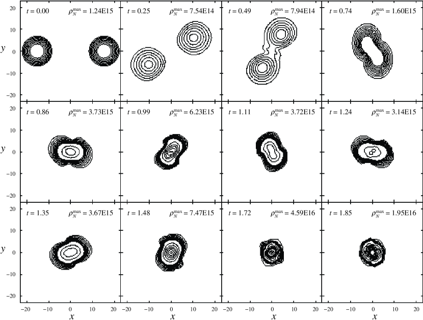
Figure 1: Density $\rho_{{}_{N}}$ on the $x$-$y$ plane. Time $t$ in units of milliseconds and the maximum of density $\rho_{{}_{N}}$ at each time are shown. Contour lines are drawn $a\times 10^{b}$g/cm³, where $a=1,2,\cdots 9$ and $b$ = 14, 15, 16. The unit of the length is $1M_{\odot}$.

We performed numerical simulations for coalescing binary neutron stars and evaluated the gravitational waves. We used $475\times 475\times 238$ Cartesian grid assuming the symmetry with respect to the equatorial plane, which require memory of about 80GBytes. The separation between grid points is $\Delta x=\Delta y=\Delta z=1M_{\odot}$, i.e., equal spacing. Here we use the units of $G=c=1$. As the initial condition, we put two spherical stars of rest mass $1.5M_{\odot}$ and radius $7.7M_{\odot}=11.6$km. The separation between the center of each mass is $30.2M_{\odot}=46.2$km. As for an equation of state, we use the ${\gamma}=2$ polytropic equation of state. The initial rotational velocity is given so that the circulation of the system vanishes approximately as

$$\vec{V}_{a}(\vec{r})=\vec{\Omega}\times\vec{r}-\vec{\Omega}\times\left(\vec{r}-\vec{r}_{a}\right),\qquad(a=1,2)$$ (104)

where $\vec{\Omega}$ is the orbital angular velocity and $\vec{r}_{a}$ is the location of the center of each star. Now we set $\Omega=0.010/M_{\odot}$, then the angular momentum $J_{0}$ becomes $6.7M_{\odot}^{2}$. The total ADM mass $M_{\mbox{\scriptsize ADM}}$ of the system is $2.76M_{\odot}$ and $q\equiv J_{0}/M_{\mbox{\scriptsize ADM}}^{2}=0.89$.

Figure 2: Plots $rh_{+,\times}$ along $z$-axis at $r=110\sim 140M_{\odot}$ as a function of $t-r$.

Figure 3: Plots $r^{3}h_{+,\times}$ as a function of $t$.

Figures 1 shows the evolution of the density $\rho_{{}_{N}}$ on the $x$-$y$ plane. The stars start to coalesce at approximately $t=0.5$msec and an almost axisymmetric star is formed by $t=1.8$msec.

Figure 3 shows the gravitational wave forms $rh_{+}$ and $rh_{\times}$ on the $z$-axis evaluated at $r=110,120,130$ and $140M_{\odot}$ as functions of the retarded time $t-r$. The lines of $rh_{+}(t-r)$ and $rh_{\times}(t-r)$ estimated at $r=110\sim 140M_{\odot}$ for $t-r>0$ coincide with each other but they don’t for $t-r<0$. Figure 3 shows $r^{3}h$ as a function of $t$. It reveals that $h$ includes a non-wave mode proportional to $r^{-3}$, which corresponds to the quadrupole part in the Newtonian potential of the background metric. It decreases fast as the merger of stars proceeds.

Therefore we eliminate the non-wave mode from $h_{+}$ and $h_{\times}$ using Fourier transformation as follows:

• Assuming that total waves are expressed as a sum of wave parts $F(t-r)/r$ and non-wave parts $G(t)/r^{3}$,

  $$h(t,r)=\frac{F(t-r)}{r}+\frac{G(t)}{r^{3}}.$$ (105)

• Fourier components of $h(t,r)$ are written as

  $$h_{\omega}(r)=\frac{e^{-\mbox{\scriptsize i}{\omega}r}}{r}F_{\omega}(r)+\frac{1}{r^{3}}G_{\omega}(r).$$ (106)

  where

  $$F_{\omega}\equiv\frac{1}{2\pi}\int F(t)e^{-\mbox{\scriptsize i}\omega t}\,\mbox{d}t$$ (107)

  and

  $$G_{\omega}\equiv\frac{1}{2\pi}\int G(t)e^{-\mbox{\scriptsize i}\omega t}\,\mbox{d}t.$$ (108)

• From the values of $h_{\omega}(r)$ in different radial coordinates $r_{1}$ and $r_{2}$, $F_{\omega}$ can be given by

  $$F_{\omega}=\frac{r_{2}^{3}h_{\omega}(r_{2})-r_{1}^{3}h_{\omega}(r_{1})}{r_{2}^{2}e^{-\mbox{\scriptsize i}\omega r_{2}}-r_{1}^{2}e^{-\mbox{\scriptsize i}\omega r_{1}}}.$$ (109)

• Fourier components $\hat{h}_{\omega}(r)$ of gravitational waves are given by

  $$\hat{h}_{\omega}(r_{k})\equiv\frac{e^{-\mbox{\scriptsize i}\omega r_{k}}}{r_{k}}F_{\omega},\quad k=1,~{}2.$$ (110)

• By inverse Fourier transformation of $\hat{h}_{\omega}(r)$, we can get the gravitational waves, which do not include non-wave modes,

  $$h_{+}(t,r)-\mbox{i}h_{\times}(t,r)=\int{\hat{h}_{\omega}(r)e^{\mbox{\scriptsize i}\omega t}}\,\mbox{d}\omega.$$ (111)

Figure 4: Wave forms $rh_{+,\times}$ along $z$-axis as a function of $t-r$. The curves are averages of $rh_{+,\times}$ estimated at $r=110\sim 200M_{\odot}$ and error bars denote $2\sigma$.

Figure 5: The comparison $h_{+,\times}$ shown in Fig.5 (solid lines)and $\widehat{h}_{+,\times}$ defined by Eqs.(112) and (113) (dashed lines).

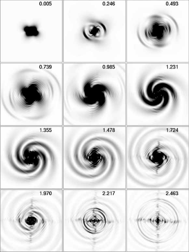
Figure 6: The propagation of the gravitational waves. “The energy densities of gravitational waves” $r^{2}\rho_{{}_{\mbox{\scriptsize GW}}}$ on the $x$-$y$ plane are shown as gray scale figures. Time in units of milliseconds is shown.

The resultant wave form is shown in Fig.5. The curves represent the average of $h_{+}$ and $h_{\times}$ calculated at $r=110,120,\cdots 200M_{\odot}$ and twice the dispersion $2\sigma$ is shown as error bars.

Figure 5 compares $h_{+}$ and $h_{\times}$ given by Eq.(111) with the metric perturbation $\widehat{h}_{+}$ and $\widehat{h}_{\times}$ defined by

$$\widehat{h}_{+}=\frac{1}{2}\left(h_{xx}-h_{yy}\right),$$ (112)

and

$$\widehat{h}_{\times}=h_{xy},$$ (113)

respectively, where $h_{ij}$ is defined by Eq.(46). Although $\widehat{h}_{+}$ and $\widehat{h}_{\times}$ include gauge dependent mode, they almost coincide with the gauge independent wave $h_{+}$ and $h_{\times}$. It shows that the gauge mode in $\widehat{h}_{+}$ and $\widehat{h}_{\times}$ is small, while it may be only accidental. However, we note that the pseudo-minimal distortion condition Eq.(42) guarantee $\sum_{j}\partial_{j}h_{ij}=0$, and thus $\widehat{h}_{+}$ and $\widehat{h}_{\times}$ are transverse-traceless. Then we can argue “the energy density of the gravitational waves” as

$$\rho_{\mbox{\scriptsize GW}}=\frac{1}{32\pi}\dot{\widetilde{\gamma}}_{ij}\dot{\widetilde{\gamma}}_{ij}=\frac{1}{32\pi}\widetilde{A}_{ij}\widetilde{A}_{ij}.$$ (114)

The propagation of $r^{2}\rho_{\mbox{\scriptsize GW}}$ is shown in Fig.6. A spiral pattern appears, which can be explained naively by the quadrupole wave pattern given by

$$r^{2}\rho_{\mbox{\scriptsize GW}}=\frac{r^{2}}{32\pi}\left(\widetilde{A}_{ij}\right)^{2}\propto\cos 2\theta+\sin^{2}\theta\,\sin^{2}\left(2\Omega(t-r)-2\phi\right)/4.$$ (115)

On the $x$-$y$ plane, where $\theta=\pi/2$, $\rho_{\mbox{\scriptsize GW}}$ is constant along the spiral of $r+\phi/\Omega$ = constant.

The gauge invariant luminosity $\mbox{d}E_{\mbox{\scriptsize GW}}/\mbox{d}t$ and the total energy $\Delta E_{\mbox{\scriptsize GW}}$ of the gravitational waves can be calculated as

$$\frac{\mbox{d}E_{\mbox{\scriptsize GW}}}{\mbox{d}t}=\frac{1}{32\pi}\sum_{l,m}\left(\left|\partial_{t}\Psi^{(e)}_{lm}(t,r)\right|^{2}+\left|\partial_{t}\Psi^{(o)}_{lm}(t,r)\right|^{2}\right)$$ (116)

and

$$\Delta E_{\mbox{\scriptsize GW}}=\int\frac{\mbox{d}E_{\mbox{\scriptsize GW}}}{\mbox{d}t}\,\mbox{d}t,$$ (117)

respectively. The luminosity and the total energy can be also estimated from Eq.(114) as

$$\frac{\mbox{d}\widetilde{E}_{\mbox{\scriptsize GW}}}{\mbox{d}t}=\int_{r\rightarrow\infty}\,r^{2}\rho_{\mbox{\scriptsize GW}}\,\mbox{d}\Omega$$ (118)

and

$$\Delta\widetilde{E}_{\mbox{\scriptsize GW}}=\int\frac{\mbox{d}\widetilde{E}_{\mbox{\scriptsize GW}}}{\mbox{d}t}\,\mbox{d}t,$$ (119)

which is not gauge invariant. The luminosity and the total energy emitted as gravitational waves up to $t$ calculated at $r=200M_{\odot}$ using Eqs.(116) and (117) as well as Eqs.(118) and (119) are plotted as functions of $t-r$ in Fig.7, which shows that Eq.(114) gives a good estimate of the energy density of the gravitational waves as expected from Fig.5.

Figure 7: The luminosity $\mbox{d}E_{\mbox{\scriptsize GW}}/\mbox{d}t$ (in units of $M_{\odot}c^{2}$/sec) and total energy $\Delta E_{\mbox{\scriptsize GW}}$ (in units of $10^{-3}M_{\odot}c^{2}$) emitted as gravitational waves up to $t$. The solid and dashed lines plot the values calculated using Eq.(116) and Eq(118), respectively. They are evaluated at $r=200M_{\odot}$.

7 Conclusion

We showed a stable code using the pseudo-minimal distortion condition and the maximal slicing condition for a coalescing neutron star binary.

Figure 8: Lapse function $\alpha$ (solid lines) and density $\rho_{{}_{N}}$ (dashed lines) along $x$-axis at $t$=0(left) and 1.72msec(right).

We were able to extract the wave form of the gravitational radiation using the gauge-invariant extraction techniques. The amplitude of the gravitational waves is

$$h\sim 1\times 10^{-21}\left(\frac{r}{\mbox{10Mpc}}\right).$$ (120)

As shown in Fig.7, the total energy emitted is

$$\Delta E_{\mbox{\scriptsize GW}}(t<3\mbox{msec})\approx 2\times 10^{-3}M_{\odot}c^{2}\approx 3\times 10^{51}\mbox{erg}\approx 0.1\%\mbox{ of }M_{\mbox{\scriptsize tot}}\,c^{2}.$$ (121)

The angular momentum lost by the gravitational waves are given by

$$\Delta J=\frac{1}{32\pi}\int\sum_{l,m}\left(\left|m\Psi^{(e)}_{lm}\,\partial_{t}\Psi^{(e)}_{lm}\right|+\left|m\Psi^{(o)}_{lm}\,\partial_{t}\Psi^{(o)}_{lm}\right|\right)\,\mbox{d}t,$$ (122)

which is $7\times 10^{-2}\,(GM_{\odot}^{2}/c)\sim$ 1% of the initial angular momentum of the system.

We have not searched an apparent horizon to see if a black hole is formed, Instead we plot $\alpha$ and $\rho_{{}_{N}}$ along the $x$-axis at $t$=0 and 1.72msec in Fig.8. The gradient of $\alpha$ near the surface of the merged star becomes large and the value gets less than 0.3. This suggests the formation of a black hole.

If the black hole is formed after the merger of two neutron stars, quasi-normal modes of the black hole are excited. To investigate a possibility that the excitation of the quasi-normal modes can be seen by the numerically calculated waves, we evaluated the energy spectrum of the gravitational waves, which is given by

$$\frac{\mbox{d}E_{\mbox{\scriptsize GW}}}{\mbox{d}\omega}=\frac{1}{32\pi}\sum_{l,m}\omega^{2}\left(\left|\Psi^{(e)}_{lm\omega}(r)\right|^{2}+\left|\Psi^{(o)}_{lm\omega}(r)\right|^{2}\right),$$ (123)

Figure 9: The energy spectrum of the gravitational waves. The curves are averages of $\mbox{d}E/\mbox{d}\omega$ estimated at $r=110\sim 200M_{\odot}$ and error bars denote $2\sigma$.

where $\Psi^{(I)}_{lm\omega}(r)$ is the Fourier transformation of $\Psi^{(I)}_{lm}(t,r)$, and is shown in Fig. 9. The frequencies of the quasi-normal modes depend on the angular momentum of the black hole, but the fundamental frequency of $l=2$ for a Schwarzschild black hole of mass $2.8M_{\odot}$ is ${\omega}=25~{}\mbox{msec}^{-1}$. A peak near this frequency appears in Fig. 9. Unfortunately, however, rotating angular frequency just when the merger of the stars finishes is $12~{}{\sim}~{}15~{}\mbox{msec}^{-1}$ and thus they will radiate the waves of frequency near ${\omega}=25~{}\mbox{msec}^{-1}$. So it is not clear whether this peak corresponds to the emission of the quasi-normal mode of the formed black hole.

Our results must be compared with the model H-1 of Shibata and Uryu.[7]. The wave form and the luminosity of the gravitational waves are qualitatively consistent, while our values of the radiated energy and angular momentum are smaller than theirs. It caused by the difference of the initial data; two stars merge more quickly in our calculation since they are not in quasi-equilibrium at the initial time. Nevertheless, the ratio of $(\Delta E_{\mbox{\scriptsize GW}}/M_{\mbox{\scriptsize ADM}})$ to $(\Delta J/J_{0})$ agrees with their discussion.

Finally, we must mention the accuracy of our code. Essential parts of code tests are summarized in Oohara and Nakamura.[1] We need not solve Eq.(26) for $K$ since we use the maximal slicing, where $K=0$, but it is solved to monitor the numerical precision. The value of $K$ is kept as small as 0.1% of a typical value of $K_{ij}$ but it becomes large from the numerical boundary region in the final stage of simulation. It is due to a small reflection of gravitational waves at the numerical boundary. Since we use the pseudo-minimal distortion condition, $\widetilde{F}^{i}=\widetilde{\gamma}^{ij}{}_{,j}$ must be zero. It is satisfied within a few % of the derivative of $\widetilde{\gamma}^{ij}$, while the error grows in the same way as $K$ in final stage of simulation. The total ADM mass is conserved within 10% error up to $t<1.7$msec. When two stars merge and a single compact object is formed, the conservation get worse, since our grid is too coarse to represent such a compact object. Since it is likely to be a black hole by that time, however, the global characteristics of gravitational radiation should be hardly affected.

We found that the gravitational waves are in small part reflected at the numerical boundary and reflected waves grow up gradually after $t\approx 2.5$msec. It is because the boundary is still too close. In reality, if the distance of the numerical boundary is halved, the growth of the reflected waves near the boundary will be visible by $t=1.4$msec in the distribution of the energy density of the gravitational waves $\rho_{{}_{\mbox{\scriptsize GW}}}$, while it is not yet visible in Fig.6. This problem must be overcome if the numerical boundary is located farther. In addition, a finer grid is required to investigate the formation of a black hole. To perform simulations with a finer and larger-sized grid, we must improve schemes for solving elliptic partial differential equations and evolution equations. The most CPU hours are consumed for solving elliptic equations for $\beta^{i}$ (Eqs.(50) and (51)), $\alpha$ (Eq.(47)) and $\phi$ (Eq.(61)), and thus the reduction of CPU hours required to solve these equations is effective. The present code requires memory of 80GBytes and 100 CPU hours with a $475\times 475\times 238$ grid. The size is not restricted by the memory but by CPU hours. Therefore, larger-scale simulations can be performed according to the speedup of the code. We are still improving the code, including implementation of new schemes and an apparent horizon finder as well as reformulation of the Einstein equations, some results of which will be presented soon.

References

- [1] K. Oohara, T. Nakamura and M. Shibata, \PTPS128,1997,183.
- [2] K. Oohara and T. Nakamura, \PTPS136,1999,270
- [3] Refer Web sites; http://tamago.mtk.nao.ac.jp/tama.html, http://www.ligo.caltech.edu/, http://www.pg.infn.it/virgo/ and http://www.geo600.uni-hannover.de/.
- [4] P. Haensel, B. Paczynski and P. Amsterdamski, \AJ375,1991,209.
- [5] M. Rees and P. Meszaros, \JLMon. Not. R. Astron. Soc.,258,1992,41.
- [6] A. Abrahams, D. Dernstein, D. Hobill and E. Seidel, \PRD45,1992,3544.
- [7] M. Shibata and K. Uryu, \PTP107,2002,265.
- [8] For example, H. Shinkai and G. Yoneda in Progress in Astronomy and Astrophysics (Nova Science Publ., 2003) and references therein.
- [9] M. Shibata and T. Nakamura, \PRD42,1995,5428.
- [10] T.W. Baumgarte and S.L. Shapiro, \PRD59,1999,064037.
- [11] T. Nakamura, K. Oohara and Y. Kojima, \PTPS90,1987,1.
- [12] K. Oohara and T. Nakamura, in Relativistic Gravitation and Gravitational Radiation (Cambridge Univ. Press, 1997), p. 309.
- [13] T. Nakamura and K. Oohara, in Numerical Astrophysics, (Kluwer Academic Publ., 1999), p. 247.
- [14] K. Oohara and T. Nakamura, in Proceedings of the Ninth Marcel Grossmann Meeting on General Relativity (World Scientific, 2002), p. 2295.
- [15] V. Moncrief, \JLAnn. Phys. (N.Y.),88,1974,322.
- [16] F. J. Zerilli, \PRL24,1970,737.
- [17] B. van Leer, \JLJ. Comput. Phys.,23,1997,276.
- [18] T. Yabe, in Computational Fluid Dynamics Review 1997 (Wiley, 1997).