Theoretical X-ray Line Profiles from Colliding Wind Binaries

Abstract

We present theoretical X-ray line profiles from a range of model colliding wind systems. In particular, we investigate the effects of varying the stellar mass-loss rates, the wind speeds, and the viewing orientation. We find that a wide range of theoretical line profile shapes is possible, varying with orbital inclination and phase. At or near conjunction, the lines have approximately Gaussian profiles, with small widths ($\mathrm{HWHM}\sim 0.1v_{\infty}$) and definite blue- or redshifts (depending on whether the star with the weaker wind is in front or behind). When the system is viewed at quadrature, the lines are generally much broader ($\mathrm{HWHM}\sim v_{\infty}$), flat-topped and unshifted. Local absorption can have a major effect on the observed profiles – in systems with mass-loss rates of a few times $10^{-6}\mbox{~{}M}_{\odot}\mbox{~{}yr}^{-1}$ the lower energy lines ($E\la 1\mbox{~{}keV}$) are particularly affected. This generally results in blueward-skewed profiles, especially when the system is viewed through the dense wind of the primary. The orbital variation of the line widths and shifts is reduced in a low inclination binary. The extreme case is a binary with $i=0\degr$, for which we would expect no line profile variation.

1 Introduction

Cherepashchuk (1976) and Prilutskii & Usov (1976) proposed that the collision of the winds in a binary of early-type stars should produce copious quantities of X-ray-producing gas. Pollock (1987) found that among the 48 Wolf–Rayet stars observed with Einstein, the binary systems tended to be a few times brighter in X-rays than single stars. There is a similar trend among the O stars observed with Einstein (Chlebowski, 1989). This provided early observational evidence for colliding wind X-ray emission.

Colliding wind binaries (CWBs) have also been studied extensively with numerical hydrodynamical simulations (e.g. Luo, McCray & Mac Low, 1990; Stevens, Blondin & Pollock, 1992; Pittard & Stevens, 1997; Pittard, 1998). These works investigated the broad-band X-ray properties, since the satellites in operation at that time had only poor spectral resolution (e.g. $E/\Delta E\sim 20$ for the ASCA SIS). Nevertheless, by comparing the variable ASCA spectrum of $\gamma^{2}$ Velorum with hydrodynamical models of the system, Stevens et al. (1996) were able to confirm that the system is indeed a CWB, and were also able to place constraints on the stars’ mass-loss rates and wind velocities. This technique has more recently been applied to the high-resolution Chandra grating spectrum of $\eta$ Carinae (Pittard & Corcoran, 2002).

The unprecedented spectral resolution offered by the Chandra LETGS and HETGS and the XMM–Newton RGS ($E/\Delta E\sim 100$–1000) gives us the opportunity to study in detail the profiles of individual X-ray lines from CWBs, enabling us to probe the very hot shocked gas in the wind-wind interaction regions. Studies of X-ray line profiles from single early-type stars have already been used to test the standard wind-shock model of X-ray production, in which instabilities due to the line-driving force give rise to shocks distributed throughout the stellar wind (Lucy & White, 1980; Lucy, 1982; Owocki, Castor & Rybicki, 1988; Feldmeier, Puls & Pauldrach, 1997). Line profile calculations based upon such models (with X-ray production effectively distributed uniformly throughout a steady-state or accelerating stellar wind) generally predict broad, blueshifted and blue-skewed line profiles (Ignace, 2001; Owocki & Cohen, 2001). However, blueshifted lines have only been observed from $\zeta$ Puppis (Kahn et al., 2001; Cassinelli et al., 2001), while the lines observed from $\delta$ Orionis (Miller et al., 2002) and $\tau$ Scorpii (Cohen et al., 2003) are far narrower than is expected from the standard wind shock model.

An analogous study of X-ray line profiles from CWBs has not yet been made. Only relatively few observations of CWBs (or suspected CWBs) with high resolution spectrometers have been published; the best examples are $\gamma^{2}$ Vel (Skinner et al., 2001) and $\eta$ Car (Corcoran et al. 2001; Pittard & Corcoran 2002; Leutenegger, Kahn & Ramsay 2003). In these works, very little attention has been paid to the line profile shapes. The Chandra HETGS spectrum of $\gamma^{2}$ Vel is dominated by emission from H- and He-like ions of Ne, Mg, Si and S. The lines are broader than the expected thermal widths ($\mathrm{HWHM}\approx 500$–700$\mbox{~{}km~{}s}^{-1}$), and there are no significant wavelength shifts (Skinner et al., 2001). The lines in the Chandra HETGS spectrum of $\eta$ Car (from H-like ions of Mg, Si and S and He-like ions of Si, S, Ca and Fe) are also not significantly shifted (Corcoran et al., 2001). No mention is made of the widths of the lines. Similarly, no mention is made of line widths or shifts in the XMM–Newton RGS spectrum of $\eta$ Car (Leutenegger et al., 2003). However, there is evidence for orbital variation of line shifts in the Chandra HETGS spectrum of WR 140 (Pollock et al., in prep.) – this will be discussed further in §4.

We present here results of theoretical calculations of X-ray line profiles from such systems The model is described in §2. The calculated profiles are presented in §3, in particular showing how the profiles vary with wind parameters and the viewing orientation. The results are discussed in §4 and summarized in §5. The line profiles presented here will ultimately be compared with X-ray spectra of CWBs, and potentially offer another tool for placing constraints on the wind parameters of such systems, as well as providing new insights into the structure of the X-ray emitting regions.

2 The model

2.1 Hydrodynamic simulations

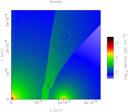
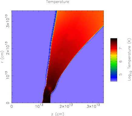
Figure 1: Density (left) and temperature (right) maps from a hydrodynamic simulation of a colliding wind binary with ${\mathcal{R}}=\sqrt{5}$ ($\dot{M}_{\mathrm{A}}=5\times 10^{-6}\mbox{~{}M}_{\odot}\mbox{~{}yr}^{-1}$, $\dot{M}_{\mathrm{B}}=1\times 10^{-6}\mbox{~{}M}_{\odot}\mbox{~{}yr}^{-1}$, $v_{\mathrm{A}}=v_{\mathrm{B}}=2000\mbox{~{}km~{}s}^{-1}$).

The hydrodynamic simulations of CWBs were carried out using vh-1, an implementation of the piecewise parabolic method (PPM; Colella & Woodward, 1984) developed by John Blondin and co-workers at the University of Virginia.

The CWBs are characterized by the wind momentum ratio ${\mathcal{R}}$, given by

$${\mathcal{R}}=\sqrt{\frac{\dot{M}_{\mathrm{A}}v_{\mathrm{A}}}{\dot{M}_{\mathrm{B}}v_{\mathrm{B}}}}$$ (1)

where $\dot{M}_{\mathrm{A}}$ and $\dot{M}_{\mathrm{B}}$ are the mass-loss rates of the stars and $v_{\mathrm{A}}$ and $v_{\mathrm{B}}$ are the terminal velocities of the winds (Stevens et al., 1992). By definition, star A (the primary) is the one with the more powerful wind (i.e. ${\mathcal{R}}\geq 1$).

Modelling the flow in a CWB is a three-dimensional problem. However, except in very close binaries, the orbital velocity of the stars is much less than the terminal velocity of the winds. Since we are not modelling close binaries, Coriolis forces are assumed to be negligible, and the problem reduces to a two-dimensional axisymmetric flow. This greatly reduces the amount of computer time needed to model the system.

It is important to note that the goal of this work is to gain insights into where different X-ray lines originate in the wind-wind collision zone, and how the profiles are affected by different wind parameters. As a result, rather than modelling specific CWBs, we have chosen wind parameters that are representative of typical systems. In particular, the stellar separation is fixed at $2\times 10^{13}\mbox{~{}cm}$ (287$\mbox{~{}R}_{\odot}$) , mass-loss rates are typically $\sim 10^{-6}$–$10^{-5}\mbox{~{}M}_{\odot}\mbox{~{}yr}^{-1}$, and wind speeds are typically 2000$\mbox{~{}km~{}s}^{-1}$.

For these wind parameters the winds can be assumed to be adiabatic, because the cooling time $t_{\mathrm{cool}}$ is large compared with $t_{\mathrm{esc}}$, the escape time from the shock region; i.e. the cooling parameter $\chi=t_{\mathrm{cool}}/t_{\mathrm{esc}}$ (Stevens et al., 1992) is large. A few simulations were carried out with radiative cooling included self-consistently. The inclusion of cooling did not significantly affect the results, and so in general it was not included at all.

A further assumption is that the winds are at their terminal velocities ($v_{\infty}$) when they collide. This assumption is valid for wide systems, since the winds of early-type stars typically reach their terminal velocities within a few stellar radii of the stellar surface. This assumption may be relaxed in the future for models of specific close binary systems, using the method described in Pittard (1998).

Fig. 1 is an example snapshot from one of the hydrodynamical simulations, showing the temperature and density structure of a CWB with ${\mathcal{R}}=\sqrt{5}$ ($\dot{M}_{\mathrm{A}}=5\times 10^{-6}\mbox{~{}M}_{\odot}\mbox{~{}yr}^{-1}$, $\dot{M}_{\mathrm{B}}=1\times 10^{-6}\mbox{~{}M}_{\odot}\mbox{~{}yr}^{-1}$, $v_{\mathrm{A}}=v_{\mathrm{B}}=2000\mbox{~{}km~{}s}^{-1}$). For these wind parameters, the cooling parameters (Stevens et al., 1992) are $\chi_{\mathrm{A}}=4.2$ and $\chi_{\mathrm{B}}=11.2$, and so the winds can indeed be assumed to be adiabatic. Note also that instabilities can be seen in the shocked gas, which may be due to either a difference in flow velocities along the two sides of the contact discontinuity between the two winds (Stevens et al., 1992) or numerical effects near the line of centres.

2.2 Line profile calculations

The method used for calculating X-ray line profiles from the hydrodynamic simulations simply involves calculating the line profile for each point on the grid and summing over the whole grid.

Thermal Doppler broadening is the dominant effect, and so each grid point is assumed to produce a Gaussian line profile whose height and width depend on the temperature of the gas at that point, and whose centre is blue- or redshifted according to the line-of-sight velocity of the gas, i.e.

$$I^{i}(v)=I_{0}^{i}\exp\left(\frac{-m(v-v_{\mathrm{los}}^{i})^{2}}{2kT^{i}}\right)$$ (2)

where $I^{i}(v)\mathrm{d}v$ is the intensity of the line from the $i$th grid point between a velocity shift of $v$ and $v+\mathrm{d}v$, $m$ is the ion mass, $T^{i}$ is the gas temperature, and $v_{\mathrm{los}}^{i}$ is the line-of-sight velocity of the gas.

The height of the Gaussian $I_{0}^{i}$ is calculated using the list of spectral lines available from the spex website. This list gives the emissivity $Q$ of a few thousand UV and X-ray lines over a range of temperatures. For an arbitrary temperature, the emissivity is calculated by interpolating between the tabulated values. If the temperature lies outside the range of temperatures for which there are data, the emissivity is assumed to be zero and the grid point is skipped over. The total line luminosity $L_{\mathrm{line}}^{i}$ for the $i$th grid point is obtained by multiplying these emissivities by $n_{\mathrm{e}}^{i}n_{\mathrm{H}}^{i}V^{i}$, where $n_{\mathrm{e}}^{i}$ and $n_{\mathrm{H}}^{i}$ are the electron and hydrogen number densities and $V^{i}$ is the volume of the emitting gas at the grid point. $L_{\mathrm{line}}^{i}$ is equal to the integral of equation (2) over all $v$, and so

$$I_{0}^{i}=Q(T^{i})n_{\mathrm{e}}^{i}n_{\mathrm{H}}^{i}V^{i}\sqrt{\frac{m}{2\pi kT^{i}}}$$ (3)

Two major assumptions have to be made in order to use the data in the spex list of lines. Firstly, the plasma is assumed to be in collisional ionization equilibrium, and secondly both winds are assumed to have solar abundances. The latter is a valid assumption for O+O binaries, but not for WR+O binaries, in which the Wolf–Rayet wind has significantly non-solar abundances. This assumption will be relaxed in the future when specific WR+O binaries are modelled.

The line profile produced by each grid point is then attenuated by photoabsorption. The absorbing column to each emitting grid point is calculated by integrating the density numerically along the line-of-sight. The density is either obtained directly from the hydrodynamic grid, or by extrapolation when off the grid. The opacities used were calculated for a solar abundance plasma using xstar. For a given line, the opacity is assumed to be constant with wavelength across the width of the line profile. Most of the absorption takes place in the cool, unshocked winds surrounding the wind-wind collision region, which are both assumed to have a temperature of $3\times 10^{4}\mbox{~{}K}$. However, opacities have also been calculated for higher temperatures ($10^{5}$, $10^{6}$, $10^{7}$ and $10^{8}\mbox{~{}K}$). The opacity of hot, shocked gas of arbitrary temperature in the wind-wind collision region is taken into account by interpolating between these values, though in fact this gas makes only a small contribution to the overall absorption. When calculating the contribution of gas off the grid to the absorption, we assume its temperature is equal to the gas temperature at the point on the line-of-sight where we leave the grid. This tends to underestimate the absorption, as it sometimes assumes that gas off the grid is hotter than it actually is. The alternative is to assume that all the gas off the grid is cold ($T=3\times 10^{4}\mbox{~{}K}$), which would tend to overestimate the absorption. However, we have found that there is generally very little difference in the resulting profiles calculated by the two methods.

The resulting line profile from the CWB is the sum of all the profiles calculated by the above method for the entire grid. Results for a range of CWB parameters are shown in the following section.

Table 1: The wavelengths of the Ly$\alpha$ lines used in this work (taken from spex list of lines). $\lambda_{1}$ and $\lambda_{2}$ are the wavelengths of the brighter and weaker components, respectively. $\Delta v$ is the difference in wavelengths expressed as a velocity shift ($\Delta v=c(\lambda_{2}-\lambda_{1})/\lambda_{1}$).

Ion	$\lambda_{1}$ (Å)		$\lambda_{2}$ (Å)		$\Delta v$ ($\mbox{~{}km~{}s}^{-1}$)
O viii	18.	971	18.	977	95
Ne x	12.	132	12.	137	124
Mg xii	8.	419	8.	424	178
Si xiv	6.	181	6.	187	291
S xvi	4.	729	4.	733	254

3 Results

Line profiles were calculated for the Ly$\alpha$ lines from the abundant elements O, Ne, Mg, Si and S. These lines are in fact closely spaced doublets; both components were included in the calculations, but other nearby lines were ignored (as their emissivities are much lower than those of the Ly$\alpha$ lines). The wavelengths of the lines are shown in Table 1.

The O to S Ly$\alpha$ lines were chosen because they feature strongly in the X-ray grating spectra of many early-type stars (Schulz et al., 2000; Waldron & Cassinelli, 2001; Kahn et al., 2001; Cassinelli et al., 2001; Miller et al., 2002). They are also insensitive to the plasma density, unlike the fir (forbidden-intercombination-resonance) triplets from He-like ions. This greatly simplifies the calculations.

3.1 Location of the line-emitting plasma

Figure 2: The fraction of the total line emission as a function of distance $p$ from the line of centres, for the Ly$\alpha$ lines from O viii (double-dashed), Ne x (dotted), Mg xii (dashed), Si xiv (dot-dashed) and S xvi (solid). The mass-loss rates are $\dot{M}_{\mathrm{A}}=5\times 10^{-6}\mbox{~{}M}_{\odot}\mbox{~{}yr}^{-1}$ and $\dot{M}_{\mathrm{B}}=1\times 10^{-6}\mbox{~{}M}_{\odot}\mbox{~{}yr}^{-1}$. The wind speeds are (a) $v_{\mathrm{A}}=v_{\mathrm{B}}=2000\mbox{~{}km~{}s}^{-1}$, (b) $v_{\mathrm{A}}=v_{\mathrm{B}}=3000\mbox{~{}km~{}s}^{-1}$. The stellar separation $D=2\times 10^{13}\mbox{~{}cm}$.

Fig. 2 shows the fraction of the total unabsorbed line emission as a function of cylindrical distance $p$ from the line of centres for each of five lines (i.e. the figure shows the fractional line luminosity from a series of thin cylindrical shells whose symmetry axes lie along the line of centres). The results in Fig. 2(a) are from a simulation with $\dot{M}_{\mathrm{A}}=5\times 10^{-6}\mbox{~{}M}_{\odot}\mbox{~{}yr}^{-1}$, $\dot{M}_{\mathrm{B}}=1\times 10^{-6}\mbox{~{}M}_{\odot}\mbox{~{}yr}^{-1}$ and $v_{\mathrm{A}}=v_{\mathrm{B}}=2000\mbox{~{}km~{}s}^{-1}$. The results in Fig. 2(b) are from a simulation with the same mass-loss rates, but with higher wind velocities (3000$\mbox{~{}km~{}s}^{-1}$). The simulations were carried out on an $8\times 10^{13}\mbox{~{}cm}$ square grid with a stellar separation $D=2\times 10^{13}\mbox{~{}cm}$. In all cases, the values of $p$ are normalized to $D$.

In both cases, one can clearly see that most of the Ly$\alpha$ emission from the lighter elements (e.g. O, Ne) originates a few times $10^{13}\mbox{~{}cm}$ from the line of centres, whereas that from heavier elements (e.g. S) originates much further in ($\sim 1\times 10^{13}\mbox{~{}cm}$ from the line of centres). This is exactly as expected, because the temperature of the plasma in the wind-wind collision region falls off with increasing $p$. In the inner regions it is too hot for O viii and Ne x to exist in large amounts (these elements are mostly fully ionized), whereas in the outer regions it is too cool to have significant amounts of H-like ions of heavier elements.

The main difference between Figs. 2(a) and 2(b) is that for the system with higher wind velocities, the line emission tends to originate from larger values of $p$. This is because the higher wind velocity results in a higher post-shock temperature.

For all the lines, the radius at which the emission peaks is smaller than the radius at which the plasma temperature equals the temperature of maximum emissivity. This is because the emissivity $Q$ of the lines varies fairly slowly with $p$. However, the $n_{\mathrm{e}}^{i}n_{\mathrm{H}}^{i}V^{i}$ term in equation (3) varies as approximately $p^{-2}$, except near the line of centres, where it turns over and tends to zero. As a result the emission originates from further in than one might naïvely expect from the temperature alone.

	${\mathcal{R}}=1$	${\mathcal{R}}=\sqrt{5}$	${\mathcal{R}}=3$
$\theta=0\degr$
$\theta=45\degr$
$\theta=90\degr$
$\theta=135\degr$
$\theta=180\degr$

Figure 3: Unabsorbed (solid) and absorbed (dashed) O viii Ly$\alpha$ line profiles for a range of wind momentum ratios ${\mathcal{R}}$ and viewing angles $\theta$. The profiles are for systems with $\dot{M}_{\mathrm{A}}=1,5,9\times 10^{-6}\mbox{~{}M}_{\odot}\mbox{~{}yr}^{-1}$, $\dot{M}_{\mathrm{B}}=1\times 10^{-6}\mbox{~{}M}_{\odot}\mbox{~{}yr}^{-1}$ and $v_{\mathrm{A}}=v_{\mathrm{B}}=2000\mbox{~{}km~{}s}^{-1}$.

	${\mathcal{R}}=1$	${\mathcal{R}}=\sqrt{5}$	${\mathcal{R}}=3$
$\theta=0\degr$
$\theta=45\degr$
$\theta=90\degr$
$\theta=135\degr$
$\theta=180\degr$

Figure 4: Unabsorbed (solid) and absorbed (dashed) Ne x Ly$\alpha$ line profiles for a range of wind momentum ratios ${\mathcal{R}}$ and viewing angles $\theta$. The profiles are for systems with $\dot{M}_{\mathrm{A}}=1,5,9\times 10^{-6}\mbox{~{}M}_{\odot}\mbox{~{}yr}^{-1}$, $\dot{M}_{\mathrm{B}}=1\times 10^{-6}\mbox{~{}M}_{\odot}\mbox{~{}yr}^{-1}$ and $v_{\mathrm{A}}=v_{\mathrm{B}}=2000\mbox{~{}km~{}s}^{-1}$.

	${\mathcal{R}}=1$	${\mathcal{R}}=\sqrt{5}$	${\mathcal{R}}=3$
$\theta=0\degr$
$\theta=45\degr$
$\theta=90\degr$
$\theta=135\degr$
$\theta=180\degr$

Figure 5: Unabsorbed (solid) and absorbed (dashed) Mg xii Ly$\alpha$ line profiles for a range of wind momentum ratios ${\mathcal{R}}$ and viewing angles $\theta$. The profiles are for systems with $\dot{M}_{\mathrm{A}}=1,5,9\times 10^{-6}\mbox{~{}M}_{\odot}\mbox{~{}yr}^{-1}$, $\dot{M}_{\mathrm{B}}=1\times 10^{-6}\mbox{~{}M}_{\odot}\mbox{~{}yr}^{-1}$ and $v_{\mathrm{A}}=v_{\mathrm{B}}=2000\mbox{~{}km~{}s}^{-1}$.

	${\mathcal{R}}=1$	${\mathcal{R}}=\sqrt{5}$	${\mathcal{R}}=3$
$\theta=0\degr$
$\theta=45\degr$
$\theta=90\degr$
$\theta=135\degr$
$\theta=180\degr$

Figure 6: Unabsorbed (solid) and absorbed (dashed) Si xiv Ly$\alpha$ line profiles for a range of wind momentum ratios ${\mathcal{R}}$ and viewing angles $\theta$. The profiles are for systems with $\dot{M}_{\mathrm{A}}=1,5,9\times 10^{-6}\mbox{~{}M}_{\odot}\mbox{~{}yr}^{-1}$, $\dot{M}_{\mathrm{B}}=1\times 10^{-6}\mbox{~{}M}_{\odot}\mbox{~{}yr}^{-1}$ and $v_{\mathrm{A}}=v_{\mathrm{B}}=2000\mbox{~{}km~{}s}^{-1}$.

	${\mathcal{R}}=1$	${\mathcal{R}}=\sqrt{5}$	${\mathcal{R}}=3$
$\theta=0\degr$
$\theta=45\degr$
$\theta=90\degr$
$\theta=135\degr$
$\theta=180\degr$

Figure 7: Unabsorbed (solid) and absorbed (dashed) S xvi Ly$\alpha$ line profiles for a range of wind momentum ratios ${\mathcal{R}}$ and viewing angles $\theta$. The profiles are for systems with $\dot{M}_{\mathrm{A}}=1,5,9\times 10^{-6}\mbox{~{}M}_{\odot}\mbox{~{}yr}^{-1}$, $\dot{M}_{\mathrm{B}}=1\times 10^{-6}\mbox{~{}M}_{\odot}\mbox{~{}yr}^{-1}$ and $v_{\mathrm{A}}=v_{\mathrm{B}}=2000\mbox{~{}km~{}s}^{-1}$.

3.2 The profiles

Figs. 3 to 7 show theoretical Ly$\alpha$ line profiles for O viii, Ne x, Mg xii, Si xiv and S xvi, respectively. The profiles have been calculated from single snapshots from the hydrodynamical simulations. The model CWBs have $\dot{M}_{\mathrm{B}}=1\times 10^{-6}\mbox{~{}M}_{\odot}\mbox{~{}yr}^{-1}$ and $v_{\mathrm{A}}=v_{\mathrm{B}}=2000\mbox{~{}km~{}s}^{-1}$; the wind momentum ratio ${\mathcal{R}}$ is adjusted by varying $\dot{M}_{\mathrm{A}}$. In all cases, profiles are shown for 3 values of ${\mathcal{R}}$ and for 5 different viewing angles $\theta$, where $\theta$ is the angle between the line-of-sight and the line-of-centres, with $\theta=0\degr$ corresponding to viewing the system from behind the secondary star. For a circular orbit, $\theta$ is related to the inclination $i$ and the orbital phase angle $\phi$ by

$$\cos\theta=\sin i\cos\phi$$ (4)

where $\phi=0\degr$ corresponds to the secondary being in front. Profiles with and without absorption by the stellar winds are shown. The wavelength shifts are calculated relative to the rest wavelength of the brighter component of the Ly$\alpha$ lines, and have been scaled to the wind velocity. The unabsorbed O viii Ly$\alpha$ line for ${\mathcal{R}}=1$ has been normalized such that its total luminosity is equal to unity. The other lines are normalized relative to this line, preserving the relative line luminosities.

The secondary components of the Ly$\alpha$ lines are only noticeable for the shorter wavelength lines. This is because the wavelength difference between the components (0.004–0.006 Å; see Table 1) corresponds to a larger velocity shift for these lines. In practice, after the lines have been folded with the instrumental response of the Chandra or XMM–Newton gratings, the two components would not be resolvable. However, including both components of the Ly$\alpha$ lines gives broader lines than one would get by considering only the brighter component.

3.3 Variation of line parameters with viewing angle and wind momentum ratio

Figure 8: Graphs showing how the mean wavelength shift, HWHM, and normalized line luminosity of the unabsorbed (solid) and absorbed (dashed) O viii Ly$\alpha$ line profile vary with viewing angle. Results for ${\mathcal{R}}=1$, $\sqrt{5}$ and 3 are represented by crosses, solid squares and open circles, respectively.

Figure 9: Graphs showing how the mean wavelength shift, HWHM, and normalized line luminosity of the unabsorbed (solid) and absorbed (dashed) Ne x Ly$\alpha$ line profile vary with viewing angle. Results for ${\mathcal{R}}=1$, $\sqrt{5}$ and 3 are represented by crosses, solid squares and open circles, respectively.

Figure 10: Graphs showing how the mean wavelength shift, HWHM, and normalized line luminosity of the unabsorbed (solid) and absorbed (dashed) Mg xii Ly$\alpha$ line profile vary with viewing angle. Results for ${\mathcal{R}}=1$, $\sqrt{5}$ and 3 are represented by crosses, solid squares and open circles, respectively.

Figure 11: Graphs showing how the mean wavelength shift, HWHM, and normalized line luminosity of the unabsorbed (solid) and absorbed (dashed) Si xiv Ly$\alpha$ line profile vary with viewing angle. Results for ${\mathcal{R}}=1$, $\sqrt{5}$ and 3 are represented by crosses, solid squares and open circles, respectively.

Figure 12: Graphs showing how the mean wavelength shift, HWHM, and normalized line luminosity of the unabsorbed (solid) and absorbed (dashed) S xvi Ly$\alpha$ line profile vary with viewing angle. Results for ${\mathcal{R}}=1$, $\sqrt{5}$ and 3 are represented by crosses, solid squares and open circles, respectively.

Figs. 8 to 12 show how line parameters vary with viewing angle for each of the five lines. Each figure shows the variation of the mean scaled wavelength shift, the half width at half maximum (HWHM), and the normalized line luminosity for the unabsorbed and absorbed line profiles for three different values of ${\mathcal{R}}$ (1, $\sqrt{5}$ and 3). The horizontal dashed lines on the HWHM graphs show the thermal Doppler widths at the temperature of maximum line emission (for comparison).

In the equal winds case (${\mathcal{R}}=1$), the unabsorbed lines are approximately symmetrical and unshifted for all viewing angles. While some slight asymmetries can be seen, these are due to numerical effects. Theoretically, the unabsorbed lines for ${\mathcal{R}}=1$ must be purely symmetrical. For ${\mathcal{R}}>1$, the lines are blueshifted when the system is viewed from the side of the secondary ($\theta<90\degr$) and redshifted when the system is viewed from the side of the primary ($\theta>90\degr$). The maximum shifts occur when $\theta=0\degr,180\degr$. This occurs because the shocked region is bent towards the secondary when ${\mathcal{R}}>1$. When the system is being viewed along the line of centres, the general motion of the shocked gas is either towards or away from the observer (depending on which end of the line of centres they are looking from), with a fairly small spread in line-of-sight velocities, resulting in quite narrow lines. However, for other viewing angles this will not be the case – some of the gas will be moving towards the observer, some will be moving tangentially to the line of sight, and some will be moving away from the observer. The result of this is broader lines with smaller shifts. The extreme case is when the system is at quadrature ($\theta=90\degr$). The unabsorbed lines are very broad ($\mathrm{HWHM}\sim v_{\infty}$), but symmetrical and unshifted, apart from the presence of the secondary component on the redward side. This is exactly as expected, owing to the cylindrical symmetry of the hydrodynamic simulation – for every ‘blob’ of plasma moving towards the observer there’s a corresponding blob on the far side of the system moving away at the same speed. For $\theta\neq 90\degr$, the velocity shift (towards the blue or the red, depending on the viewing orientation) increases with ${\mathcal{R}}$, because the shocked region is bent more towards or away from the observer.

In all cases, the HWHMs are considerably larger than the typical thermal widths, indicating that the line broadening is due to a wide range of line-of-sight velocities in the bulk motion of the hot gas, rather than merely being due to simple thermal Doppler broadening.

The line luminosities increase with ${\mathcal{R}}$, because a larger $\dot{M}$ leads to a denser X-ray emitting plasma. However, for a given ${\mathcal{R}}$ the unabsorbed line luminosities do not vary with $\theta$, since these depend on the amount of hot plasma on the hydrodynamical grid, which is independent of viewing angle.

The above discussion pertains only to the unabsorbed line profiles. From the figures one can clearly see that absorption has a much more significant effect on the longer wavelength lines, such as the O viii and Ne x Ly$\alpha$ lines. This is because the continuum opacity in the cold stellar winds increases with wavelength. The opacity at the wavelength of the O viii Ly$\alpha$ line is 27.5 times that at the wavelength of the S xvi Ly$\alpha$ line. This outweighs the fact that the longer wavelength lines originate from the cooler shocked gas far from the line of centres, and so travel through less dense regions of the stellar winds.

In general, the inclusion of absorption results in blueward-skewed lines. This is because the gas that is moving away from the observer is generally on the far side of the system, and so suffers more absorption. Indeed, for $\theta\neq 0\degr,180\degr$, the velocity shift of the absorbed line is always more towards the blue than the corresponding unabsorbed line, though when the system is viewed from the side of the primary, the lines retain a mean redshift. This is because when the shocked region is bent away from the observer, there is very little blueshifted emission at all, and so the fact that redshifted emission is more strongly attenuated than blueshifted emission is less important. The range of viewing angles over which one expects to see redshifted emission is larger for the shorter wavelength lines, because absorption is less important for these lines. One would expect to see redshifted O viii Ly$\alpha$ emission for $\theta\ga 140\degr$, whereas the S xvi Ly$\alpha$ line is redshifted when $\theta\ga 90\degr$.

The HWHMs of the absorbed lines are generally either very similar to those of the corresponding unabsorbed lines, or considerably smaller (there is very little middle ground). The latter case generally occurs for the O viii line when $\theta\approx 45\degr$–$75\degr$ or $\theta\ga 90\degr$, and for the Ne x line when $\theta\ga 90\degr$ (though the HWHMs of the absorbed and unabsorbed lines are again very similar as $\theta$ approaches 180°). It also occurs to a lesser extent for the Mg xii line when $\theta\approx 110\degr$–$150\degr$. This narrowing of the absorbed lines occurs because of the higher opacity at the wavelengths of these lines. The profiles have their redward emission strongly attenuated, particularly when ${\mathcal{R}}>1$ and the system is being viewed through the dense wind of the primary ($\theta\ga 90\degr$). If it is attenuated to less than half the peak value of the blueward emission, only the blueshifted peak will contribute to the HWHM. This results in a considerably smaller HWHM, though the lines do have large redward tails. However, it is worth noting that in practice such redward tails may not by observable (they may be lost in the underlying continuum), and so the dominant observational signature would be a blueshift rather than a broadening. On the other hand, if the redward emission is not that strongly attenuated, the HWHM will be approximately equal to that of the unabsorbed line. This is generally the case for the Si xiv and S xvi lines.

The luminosities of the absorbed lines decrease with $\theta$ for ${\mathcal{R}}>1$. This is simply because as $\theta$ increases, one changes from observing the system through the wind of the secondary to observing it through the denser wind of the primary.

3.4 Lines from systems with different wind parameters but same ${\mathcal{R}}$

Figs. 13 and 14 compare how the mean scaled wavelength shift and HWHM vary with angle for systems with ${\mathcal{R}}=\sqrt{5}$ but different wind parameters. Results are shown for the O viii and S xvi Ly$\alpha$ lines, which are at the two extremes of wavelength studied here.

Fig. 13 compares lines from systems with the same wind speeds but mass-loss rates that differ by an order of magnitude. For both lines there is no difference in the shapes of the unabsorbed profiles between the two systems, though the lines from the system with the larger mass-loss rates are brighter. However, the system with the higher mass-loss rates gives an absorbed O viii line that is narrower and more blueshifted. This is because this system has denser winds, and so the line suffers more attenuation (especially the redward emission). On the other hand the S xvi line is not as strongly affected by absorption, and so there is very little difference between the two systems.

For a given ${\mathcal{R}}$, the effect of increasing the mass-loss rates on the observed (i.e. absorbed) line luminosities is a combination of two competing effects. The intrinsic line luminosity increases as $\dot{M}^{2}$, whereas the column density increases as $\dot{M}$. This means that the observed line luminosity scales as $\dot{M}^{2}\mathrm{e}^{-\alpha\dot{M}}$, where $\alpha$ is a constant that depends on $\theta$ and the opacity for the line in question. For the systems described here, we find that the observed line luminosity always increases with increasing $\dot{M}$ (for all lines and for all $\theta$). However, for larger mass-loss rates (few times $10^{-5}\mbox{~{}M}_{\odot}\mbox{~{}yr}^{-1}$) the increasing absorption starts to dominate, and when $\theta\approx 180\degr$ (which is when the column density is largest) the observed luminosities of the longer wavelength lines start to decrease with increasing $\dot{M}$.

Fig. 14 compares the same two lines from systems with the same mass-loss rates but different wind velocities. Once the wavelength shift and the HWHM have been scaled to the wind velocity, there is very little difference between the two systems. The O viii line is generally slightly more blueshifted for the system with the lower wind velocity (since, for the same mass-loss rate, this results in a denser wind and so more absorption). On the other hand, the wavelength shift of the S xvi  line (whether to the blue to the red) is smaller for the system with the lower wind velocity. This may be because the lower wind speed results in a lower post-shock temperature, and so the line forms nearer the line of centres for this system. The shocked region is less bent towards (away from) the observer near the line of centres, resulting in a smaller blueshift (redshift) as $\theta$ approaches 0° (180°).

3.5 Time variability

Eddies/swirls in the shocked gas are frequently seen in the hydrodynamical simulations of the CWBs used for this work. These travel from the line of centres to the edge of the grid (typically $3.4\times 10^{13}\mbox{~{}cm}$ from the line of centres) on a time-scale of $\sim 200\mbox{~{}ks}$. These swirls may be due to either instabilities along the contact discontinuity between the two winds (Stevens et al., 1992) or numerical effects near the line of centres.

In order to investigate whether these swirls have any significant effect on the results, we have compared line profiles generated from snapshots of the hydrodynamical simulations separated by $\sim 25\mbox{~{}ks}$. Over the course of 10 such snapshots, we find that the calculated wavelength shifts, HWHMs and line luminosities typically vary by only a few per cent. This suggests that any observed time variability in the line profiles will be due to changes in the viewing orientation (because of the orbital motion), rather than to instabilities, etc. in the shocked gas.

Figure 13: Graphs showing how the mean wavelength shift and HWHM of the unabsorbed (solid) and absorbed (dashed) O viii and S xvi Ly$\alpha$ lines vary as a function of viewing angle for two different systems with ${\mathcal{R}}=\sqrt{5}$. The solid squares show results for a system with $\dot{M}_{\mathrm{A}}=5\times 10^{-6}\mbox{~{}M}_{\odot}\mbox{~{}yr}^{-1}$, $\dot{M}_{\mathrm{B}}=1\times 10^{-6}\mbox{~{}M}_{\odot}\mbox{~{}yr}^{-1}$ and $v_{\mathrm{A}}=v_{\mathrm{B}}=2000\mbox{~{}km~{}s}^{-1}$. The crosses show results for a system with $\dot{M}_{\mathrm{A}}=5\times 10^{-7}\mbox{~{}M}_{\odot}\mbox{~{}yr}^{-1}$, $\dot{M}_{\mathrm{B}}=1\times 10^{-7}\mbox{~{}M}_{\odot}\mbox{~{}yr}^{-1}$ and $v_{\mathrm{A}}=v_{\mathrm{B}}=2000\mbox{~{}km~{}s}^{-1}$.

Figure 14: Graphs showing how the mean wavelength shift and HWHM of the unabsorbed (solid) and absorbed (dashed) O viii and S xvi Ly$\alpha$ lines vary as a function of viewing angle for two different systems with ${\mathcal{R}}=\sqrt{5}$. The solid squares show results for a system with $\dot{M}_{\mathrm{A}}=5\times 10^{-6}\mbox{~{}M}_{\odot}\mbox{~{}yr}^{-1}$, $\dot{M}_{\mathrm{B}}=1\times 10^{-6}\mbox{~{}M}_{\odot}\mbox{~{}yr}^{-1}$ and $v_{\mathrm{A}}=v_{\mathrm{B}}=2000\mbox{~{}km~{}s}^{-1}$. The open circles show results for a system with $\dot{M}_{\mathrm{A}}=5\times 10^{-6}\mbox{~{}M}_{\odot}\mbox{~{}yr}^{-1}$, $\dot{M}_{\mathrm{B}}=1\times 10^{-6}\mbox{~{}M}_{\odot}\mbox{~{}yr}^{-1}$ and $v_{\mathrm{A}}=v_{\mathrm{B}}=3000\mbox{~{}km~{}s}^{-1}$.

3.6 Simulations of observed profiles

We have carried out some Monte Carlo simulations of observed line profiles from CWBs. Firstly, a theoretical profile is convolved with a Gaussian, which is a good first order approximation to the Chandra HETGS line response function (Chandra Proposers’ Observatory Guide, ver. 5.0, §8.2.2). The width of the Gaussian used is appropriate for the wavelength of the line in question. This convolved profile is then used as a probability distribution function in the Monte Carlo simulations. For the purposes of these simple calculations, the background/continuum emission in the vicinity of the line is assumed to negligible.

Fig. 15 shows the results of simulated observed Mg xii Ly$\alpha$ line profiles from a CWB with ${\mathcal{R}}=\sqrt{5}$ for three different viewing angles ($\theta=0\degr$, 45°, 90°). In each case there are assumed to be 200 photons in the line. The results have been binned up to 0.01 Å. These results indicate that the features described in §3.3 should easily be detectable by the Chandra HETGS: near conjunction ($\theta=0\degr$ or 180°) the lines are narrow with measurable blue- or redshifts, whereas near quadrature ($\theta=90\degr$) the profiles are very broad and fairly flat-topped with negligible wavelength shifts. Note that for this system $v_{\mathrm{A}}=v_{\mathrm{B}}=2000\mbox{~{}km~{}s}^{-1}$, corresponding to $\Delta\lambda=0.056\mbox{~{}\AA}$. Hence, near quadrature the HWHM of the observed line is an appreciable fraction of the wind velocity, as expected. Note also that the photon statistics and the instrumental response can result in an observed profile that is distinctly different from the theoretical profile for low counts: compare the middle panel of Fig. 15 with the appropriate profile in Fig. 5.

Figure 15: Simulated Mg xii Ly$\alpha$ profiles as would be observed by the Chandra HETGS-HEG. The profiles are for a system with ${\mathcal{R}}=\sqrt{5}$ ($\dot{M}_{\mathrm{A}}=5\times 10^{-6}\mbox{~{}M}_{\odot}\mbox{~{}yr}^{-1}$, $\dot{M}_{\mathrm{B}}=1\times 10^{-6}\mbox{~{}M}_{\odot}\mbox{~{}yr}^{-1}$, $v_{\mathrm{A}}=v_{\mathrm{B}}=2000\mbox{~{}km~{}s}^{-1}$) observed from three different viewing angles ($\theta=0\degr$, 45°, 90°). There are 200 photons in the line in each case. The dashed vertical line shows the rest wavelength of the brighter component of the line (see Table 1).

4 Discussion

We have seen that X-ray lines from CWBs show significant variation of wavelength shift and width as a function of viewing orientation, which is itself a function of orbital phase and inclination. The observation of phase-locked variation in the X-ray line profiles would therefore provide convincing evidence for X-ray emission from a colliding wind region. In this respect, an eclipsing binary would be the most interesting system, since during the course of its orbit the full range of viewing angles discussed above would be observed. In contrast, a system with an inclination of 0° would always be observed at $\theta=90\degr$. Any phase-locked variation in this case would just be associated with a change in orbital separation and hence the density of the shocked gas. This would probably just manifest itself as a change in line luminosity, not as a change in line shift or width.

Line profiles that vary during the orbit of a CWB have already been observed in the Chandra spectra of WR 140 (Pollock et al., in prep.). The first observation was taken just before periastron at an orbital phase of 1.982 according to the ephemeris of Williams et al. (1990). At this phase the wind collision region is bent approximately towards the observer (see White & Becker (1995) for a diagram of WR 140’s orbit), and the lines are significantly blueshifted, as would be expected. The second observation was taken just after periastron at a phase of 2.027. Although there are considerably fewer counts in this second spectrum, the lines are clearly much broader, and there is also some evidence of redshifts. While we have not compared in detail our theoretical profiles with the spectra of WR 140, these observations seem to provide at least a qualitative confirmation of some of our general predictions.

A more detailed comparison of our model line profiles with observed high-resolution X-ray spectra of CWBs may enable us to place constraints on certain parameters of the system. In practice, one would just fit to the shifts and widths of the lines, and scale the luminosities of the theoretical lines to the observed luminosities. (This approach of fitting the line shapes, not the luminosities, has already been used by Kramer, Cohen & Owocki (2003) to model the line emission from the single O star $\zeta$ Pup.) For a CWB, the main parameters would be the wind momentum ratio ${\mathcal{R}}$ and the viewing angle $\theta$, although it may also be possible to place constraints on the individual wind parameters. For this method to be effective, one would want to fit as many lines as possible simultaneously. While we have only presented results for Ly$\alpha$ lines here, the method described could be used for any line that is not affected by the density (e.g. Ly$\beta$ and Ly$\gamma$ lines, and the resonant component of the fir triplets from He-like ions).

The model presented here for calculating X-ray line profiles from CWBs is fairly simple, but it contains the essential physics and gives an overview of how the profiles vary with wind parameters and viewing angle. When the model comes to be applied to real systems, extra physics will be included in the calculations as is appropriate for the systems in question. This could include modifying the hydrodynamical simulations (e.g. radiative cooling for systems with small orbital separations and/or large mass-loss rates (Stevens et al., 1992) or radiative driving for close systems (Pittard, 1998)), or modifying the actual line profile calculations (e.g. taking into account non-solar abundances for WR+O binaries).

5 Summary

We have presented theoretical X-ray line profiles from model colliding wind systems for a range of mass-loss rates, wind velocities and viewing angles. A wide range of profile shapes is possible, varying with orbital inclination and phase.

For a high inclination binary with ${\mathcal{R}}>1$ there is a general blue/redshift at phases 0 and 0.5 (i.e. at the two conjunctions). The profiles are narrow ($\mathrm{HWHM}\sim 0.1v_{\infty}$) and approximately Gaussian. By contrast, at quadrature the profiles are generally very broad ($\mathrm{HWHM}\sim v_{\infty}$), flat-topped and unshifted. Local absorption has a major effect on the observed profiles. When a system with relatively large mass-loss rates (few times $10^{-6}\mbox{~{}M}_{\odot}\mbox{~{}yr}^{-1}$) is viewed through the dense wind of the primary, the lines are generally skewed towards the blue. This is because the redshifted emission is strongly attenuated. This effect is most noticeable for the lower energy lines ($E\la 1\mbox{~{}keV}$). These blueward-skewed profiles generally have large redward tails. In practice these tails may not be observable, and so the line would be seen as fairly narrow and blueshifted, rather than broad and blueward-skewed.

A binary with a low orbital inclination will exhibit less orbital variation of line width and shift, the extreme case being a binary with $i=0\degr$, for which we would expect no orbital variation in the line profile.

After the line shifts and widths have been scaled to the wind velocity, there is very little difference between the results from systems with $v_{\mathrm{A}}=v_{\mathrm{B}}=2000\mbox{~{}km~{}s}^{-1}$ and with $v_{\mathrm{A}}=v_{\mathrm{B}}=3000\mbox{~{}km~{}s}^{-1}$. The former systems have denser winds for the same mass-loss rate, and hence absorption has a larger effect. However, it does not significantly affect the results.

Simple Monte Carlo simulations of observed X-ray line profiles show that the features discussed above will be detectable in good Chandra HETGS spectra of CWBs. Comparing our theoretical profiles with such spectra potentially offers another method for determining the wind parameters of CWBs, and may also give us new insights into the structure of the wind-wind collision regions.

References

- Cassinelli et al. (2001) Cassinelli J. P., Miller N. A., Waldron W. L., MacFarlane J. J., Cohen D. H., 2001, ApJ, 554, L55
- Cherepashchuk (1976) Cherepashchuk A. M., 1976, SvA Lett., 2, 138
- Chlebowski (1989) Chlebowski T., 1989, ApJ, 342, 1091
- Cohen et al. (2003) Cohen D. H., de Messières G. E., MacFarlane J. J., Miller N. A., Cassinelli J. P., Owocki S. P., Liedahl D. A., 2003, ApJ, 586, 495
- Colella & Woodward (1984) Colella P., Woodward P. R., 1984, J. Comput. Phys., 54, 174
- Corcoran et al. (2001) Corcoran M. F. et al., 2001, ApJ, 562, 1031
- Feldmeier et al. (1997) Feldmeier A., Puls J., Pauldrach A. W. A., 1997, A&A, 322, 878
- Ignace (2001) Ignace R., 2001, ApJ, 549, L199
- Kahn et al. (2001) Kahn S. M., Leutenegger M. A., Cottam J., Rauw G., Vreux J.-M., den Boggende A. J. F., Mewe R., Güdel M., 2001, A&A, 365, L312
- Kramer et al. (2003) Kramer R. H., Cohen D. H., Owocki S. P., 2003, ApJL, submitted (astro-ph/0211550)
- Leutenegger et al. (2003) Leutenegger M. A., Kahn S. M., Ramsay G., 2003, ApJ, 585, 1015
- Lucy (1982) Lucy L. B., 1982, ApJ, 255, 286
- Lucy & White (1980) Lucy L. B., White R. L., 1980, ApJ, 241, 300
- Luo et al. (1990) Luo D., McCray R., Mac Low M.-M., 1990, ApJ, 362, 267
- Miller et al. (2002) Miller N. A., Cassinelli J. P., Waldron W. L., MacFarlane J. J., Cohen D. H., 2002, ApJ, 577, 951
- Owocki et al. (1988) Owocki S. P., Castor J. I., Rybicki G. B., 1988, ApJ, 335, 914
- Owocki & Cohen (2001) Owocki S. P., Cohen D. H., 2001, ApJ, 559, 1108
- Pittard (1998) Pittard J. M., 1998, MNRAS, 300, 479
- Pittard & Corcoran (2002) Pittard J. M., Corcoran M. F., 2002, A&A, 383, 636
- Pittard & Stevens (1997) Pittard J. M., Stevens I. R., 1997, MNRAS, 292, 298
- Pollock (1987) Pollock A. M. T., 1987, ApJ, 320, 283
- Prilutskii & Usov (1976) Prilutskii O. F., Usov V. V., 1976, SvA, 20, 2
- Schulz et al. (2000) Schulz N. S., Canizares C. R., Huenemoerder D., Lee J. C., 2000, ApJ, 545, L135
- Skinner et al. (2001) Skinner S. L., Güdel M., Schmutz W., Stevens I. R., 2001, ApJ, 558, L113
- Stevens et al. (1992) Stevens I. R., Blondin J. M., Pollock A. M. T., 1992, ApJ, 386, 265
- Stevens et al. (1996) Stevens I. R., Corcoran M. F., Willis A. J., Skinner S. L., Pollock A. M. T., Nagase F., Koyama K., 1996, MNRAS, 283, 589
- Waldron & Cassinelli (2001) Waldron W. L., Cassinelli J. P., 2001, ApJ, 548, L45
- White & Becker (1995) White R. L., Becker R. H., 1995, ApJ, 451, 352
- Williams et al. (1990) Williams P. M., van der Hucht K. A., Pollock A. M. T., Florkowski D. R., van der Woerd H., Wamsteker W. M., 1990, MNRAS, 243, 662