Enhancement of the helium resonance lines in the solar atmosphere by suprathermal electron excitation II: non-Maxwellian electron distributions

Abstract

In solar euv spectra the He i and He ii resonance lines show unusual behaviour and have anomalously high intensities compared with other transition region lines. The formation of the helium resonance lines is investigated through extensive non-LTE radiative transfer calculations. The model atmospheres of Vernazza, Avrett & Loeser (1981) are found to provide reasonable matches to the helium resonance line intensities but significantly over-estimate the intensities of other transition region lines. New model atmospheres have been developed from emission measure distributions derived by Macpherson & Jordan (1999), which are consistent with SOHO observations of transition region lines other than those of helium. These models fail to reproduce the observed helium resonance line intensities by significant factors. The possibility that non-Maxwellian electron distributions in the transition region might lead to increased collisional excitation rates in the helium lines is studied. Collisional excitation and ionization rates are re-computed for distribution functions with power law suprathermal tails which may form by the transport of fast electrons from high temperature regions. Enhancements of the helium resonance line intensities are found, but many of the predictions of the models regarding line ratios are inconsistent with observations. These results suggest that any such departures from Maxwellian electron distributions are not responsible for the helium resonance line intensities.

1 Introduction

The resonance lines of He i and He ii show unusual behaviour when compared with other strong emission lines in solar euv spectra. Recent results from the Solar and Heliospheric Observatory (SOHO) show that their intensities in coronal holes are factors of 1.5–2.0 smaller than in the quiet Sun (Peter 1999; Jordan, Macpherson & Smith 2001), while other lines formed at similar temperatures show only very small reductions in intensity. In the quiet Sun, the helium resonance line intensities are at least an order of magnitude too large to be reproduced by emission measure distributions that account for other transition region (TR) lines (Macpherson & Jordan 1999 – hereafter MJ99). For discussions of earlier observations of the helium resonance lines and attempts to explain them see Hammer [Hammer 1997] and MJ99. The discrepancies between observations and modelling of the helium lines in the quiet Sun have been taken to imply that some process preferentially enhances the helium resonance line intensities with respect to other lines formed in the transition region in the quiet Sun, and that the enhancement is reduced in coronal holes.

Current evidence suggests that in the quiet Sun the He ii, and to a lesser extent the He i, resonance lines are formed mainly by collisional excitation (see Smith & Jordan 2002 – hereafter Paper I – for supporting references). Because the helium resonance lines have unusually large values of $W/kT_{\textrm{e}}$, where $W$ is the excitation energy and $T_{\textrm{e}}$ is the electron temperature, their collisional contribution functions are sensitive to excitation by suprathermal electrons. He i and He ii also have long ionization times compared with other transition region species, which may allow departures from ionization equilibrium in helium. Any process exposing helium ions to larger populations of suprathermal electrons than in equilibrium will tend to increase the collisional excitation rates of the helium lines, while lines with smaller $W/kT_{\textrm{e}}$ will be relatively unaffected. MJ99 reported that attempts to model such effects had been generally unsuccessful in explaining the helium resonance line emission relative to other transition region (TR) lines. While a conclusive explanation is still lacking, some recent work appears promising (see Paper I).

Fontenla, Avrett & Loeser [Fontenla et al. 2002] have extended their earlier work [Fontenla et al. 1993], performing radiative transfer calculations for hydrogen and helium including the effects of mass-conserving flows as well as ambipolar diffusion and departures from ionization equilibrium. His preliminary results show improved agreement with observations, outflows (of 5–10 km s^-1 at $T=10^{5}$ K) producing increases in intensity in the He i and He ii resonance lines of up to an order of magnitude. Inflow models produce self-reversals in the He i 584.3-Å line, whereas observations show the line is more likely to be self-reversed in cell interior regions (e.g. MJ99) where the line shows a blue shift [Peter 1999]. This implies that the models do not yet include all relevant processes. As the models do not include the effects of diffusion on any elements heavier than helium, it is also uncertain as to how successful they will be in explaining the helium line intensities relative to other transition region lines.

Jordan (1975,1980) suggested two possible enhancement mechanisms dependent on the magnitude of the temperature gradient that might explain the coronal hole/quiet Sun contrast, Munro & Withbroe [Munro & Withbroe 1972] having found d$T/$d$h$ to be an order of magnitude smaller inside coronal holes. The first involves the transport of helium ions up the steep TR temperature gradient, allowing them to be excited at electron temperatures higher than those in equilibrium. Jordan (1980) found that intensity enhancements of up to a factor of 5 could be produced in the He ii 303.8-Å line in the quiet Sun, and a more detailed study by Andretta et al. (2000) suggests similar factors. A further investigation of the process using an improved treatment of the excitation times of the helium ions is reported in Paper I. The analysis was extended to include estimates of the effects on the He i 584.3-Å and 537.0-Å lines. We conclude, as did Andretta et al. [Andretta et al. 2000] for the He ii line, that current observations are consistent with the process accounting for at least part, and perhaps all, of the enhancement apparently required in the helium resonance lines in the quiet Sun.

A complementary study of the other of Jordan’s (1980) suggestions, enhanced collisional excitation by suprathermal electrons of non-local origin, is presented in this paper. Radiative transfer codes usually assume that the electron velocity distribution functions (EVDFs) are Maxwellian throughout the model atmospheres, but observations of the solar wind (e.g. Scudder 1994) and numerical studies of the form of the EVDF in the solar transition region suggest that significant departures from Maxwellian distributions may occur. This may result from some acceleration process maintaining a non-Maxwellian distribution in the low TR or chromosphere (Scudder 1992a; Viñas, Wong & Klimas 2000) or from the transport of high energy electrons from the upper TR and corona [Shoub 1983, Ljepojevic & Burgess 1990]. In the second case at least, the influence of the suprathermal electrons would depend on the temperature gradient.

The presence of an enhanced suprathermal electron population would simulate an increase in electron temperature in transitions with excitation energies well above the local thermal energy, and hence lead to larger excitation rates. Transitions with $W$ smaller than the energy at which the suprathermal electron population becomes important would not be affected significantly. Postulated non-Maxwellian EVDFs generally show departures from the local Maxwellian distribution which increase monotonically with energy, so that their effects on ionization rates can be even larger than on line excitation. Essentially the same effect limits the effectiveness of non-thermal transport of helium at temperatures much higher than those of normal line formation. In the case of collisional ionization by non-local suprathermal electrons the effect is a shift of the ionization equilibrium; increased collisional ionization rates raise the population of each ion at lower temperatures. Emission could therefore be increased because it would occur over a larger, more dense region.

In a study of Si iii emission line ratios, Pinfield et al. [Pinfield et al. 1999] claim to have observed both an enhancement of the intensity of the line with the largest value of $W/kT$ and a reduction in peak line formation temperature in the quiet Sun with respect to a coronal hole. In light of the above discussion, this is evidence of excitation by an enhanced suprathermal population of electrons whose importance depends on the temperature gradient in the transition region.

Although the same mechanism has often been suggested to explain the anomalous intensities of the helium resonance lines, few detailed calculations of the possible effects on helium have been made, perhaps because of the difficulty of solving the Boltzmann equation for the EVDF and the equation of radiative transfer simultaneously. Shoub [Shoub 1983] computed non-Maxwellian collision rates for the ionization of He i and He ii and the excitation of the 584.3-Å and 303.8-Å lines, but did not calculate line intensities for comparison with observations. Anderson, Raymond & Ballegooijen [Anderson et al. 1996] computed intensities for the He ii 303.8-Å line using non-Maxwellian EVDFs, but did not include radiative transfer, and made no study of He i.

In this paper I present the results of radiative transfer calculations for cases of both Maxwellian and non-Maxwellian collisional excitation. The former illustrate the problems found in attempting to model the formation of the helium resonance lines; the latter are used in a study of the observable effects that non-Maxwellian EVDFs might have on He i and He ii lines. The calculations allow an extensive comparison of the predictions of the enhanced excitation mechanism with observations. The atomic and atmospheric models used in the radiative transfer calculations are described in Section 2, and the results of radiative transfer calculations performed with Maxwellian collision rates are presented in Section 3. Section 4 describes how the effects of non-local electrons are simulated. The results of these latter calculations are presented and discussed in Section 5, and the conclusions are summarized in Section 6.

2 Atomic and atmospheric models

The radiative transfer modelling of the solar helium spectrum was carried out using version 2.2 of the multi code [Scharmer & Carlsson 1985, Carlsson 1986]. This code may be used to solve non-LTE problems in semi-infinite plane-parallel one dimensional model atmospheres. In order to calculate an emergent spectrum, the code requires a model atom, a model atmosphere, and a set of abundances (which are used to calculate background opacities - these are generally computed assuming LTE, but in the calculations reported here, the opacity due to hydrogen was computed in non-LTE). It also allows the specification of the coronal radiation field as a boundary condition at the upper edge of the model atmosphere.

2.1 The model atom

The atomic model used in this study comprises 29 bound levels of He i ($1snl~{}^{1,3}L$ terms with principal quantum number $n\leq 5$), six bound levels of He ii with $n\leq 6$, and the He iii ground state. The atomic data used before modifications were made to incorporate collisional excitation and ionization by non-Maxwellian EVDFs are listed below.

The He i part of the model was initially based on the 30 level He i model of Andretta & Jones [Andretta & Jones 1997], but using newer and/or more complete data for some of the parameters, and was extended to include He ii. Greater detail was included in the neutral stage, in order to facilitate investigation of the relationships between the 584.3-Å and 537.0-Å lines, which have been observed extensively with SOHO. Previous work by Hearn [Hearn 1969] and Andretta & Jones (1997) suggested that the formation of these lines depends on a combination of collisional and radiative transitions between many levels, and is not necessarily dominated by either direct collisional excitation or photoionization-recombination (PR). It was therefore important to include as many levels and processes as possible in this part of the model. In He ii most attention was paid to the 303.8-Å resonance line, which also appears in SOHO cds spectra.

The energies of the He i levels are taken from Martin [Martin 1987], averaging over the fine structure in the triplet levels. The fine structure in the triplet terms is not included, which is a valid approximation in the rate equations since the energy separation of the sub-levels is small enough for collisional transitions between them to keep their populations in the proportions of their statistical weights. As noted by Andretta & Jones (1997), although this assumption may not be valid in the $2p$ ${}^{3}P^{o}$ term, where the separation of the $J$-states is greatest, radiative transitions will also tend to populate the sub-levels in the same proportions in the conditions encountered in the atmospheric models used. The energies of the He ii levels are from Kisielius, Berrington & Norrington [Kisielius et al. 1996] for $n\leq 4$, from Bashkin & Stoner [Bashkin & Stoner 1975] for $n\geq 5$. States of different $l$ were summed over according to their statistical weights.

Oscillator strengths for most of the allowed transitions in He i are provided by Drake [Drake 1996], while values for the few transitions not covered there are taken from Theodosiou [Theodosiou 1987]. The rate for the spin-forbidden electric dipole $1s2p$ ${}^{3}P_{1}$ – $1s^{2}$ ${}^{1}S$ transition is taken from Drake & Dalgarno [Drake & Dalgarno 1969], and the two photon rate for the $1s2s$ ${}^{1}S$ – $1s^{2}$ ${}^{1}S$ transition is also included, from Bassani & Vignale [Bassani & Vignale 1982]. The He ii oscillator strengths are taken to be hydrogenic, using the results of Wiese, Smith & Glennon [Wiese et al. 1966].

Stark broadening parameters for He i are from Dimitrijević & Sahal-Bréchot (1984,1990) where available, with the remainder being estimated using the formula of Freudenstein & Cooper (1978). The Stark widths of Griem [Griem 1974] are used for He ii. Van der Waals broadening is treated using the tables of Deridder & Van Rensbergen [Deridder & Van Rensbergen 1976], taking advantage of alterations made to multi by Rowe [Rowe 1996].

For most of the levels of He i photoionization cross-sections are drawn from the Opacity Project database [Seaton 1987]; they were calculated by Fernley, Taylor & Seaton [Fernley et al. 1987]. The broadest, most prominent resonances in the cross-sections are represented approximately in the model, particularly in the resonance continuum, as there is some variation of the coronal radiation field in the wavelength range of the resonances. The 4 ${}^{3}P$, 4 ${}^{1,3}F$, 5 ${}^{3}P$, 5 ${}^{1,3}F$, and 5 ${}^{1,3}G$ levels of He i are treated as hydrogenic, as are the photoionization cross-sections for He ii [Menzel & Pekeris 1935].

Photoionization is important in establishing the ionization balance between all three stages of helium and is important in the formation of some of its lines. The effects of coronal radiation shortwards of 504 Å are therefore included in the calculation of ionization and recombination rates. The coronal illumination was represented using the solar EUV irradiance model of Tobiska (1991,1993). The spectrum of radiation at minimum coronal activity was used to give incoming intensities at the solar surface representative of the average quiet corona. Photoionization of He i occurs directly from the ground state, by coronal radiation, and by a two-stage process, in which He i triplet states, collisionally excited from the ground, are rapidly photoionized (directly or by successive photoexcitations followed by ionization) by the photospheric radiation field. The importance of this two-stage process was recognized in early calculations by Athay & Johnson [Athay & Johnson 1960] and Hearn [Hearn 1969], and by Andretta & Jones [Andretta & Jones 1997], who emphasized how the singlet and triplet systems of He i have quite different roles in the ionization balance. Collisional excitation of singlet levels tends to lead more often to decays back to the ground, to which the singlet levels are strongly connected by the allowed radiative transitions $1snp$ ${}^{1}P^{o}$ – $1s^{2}$ ${}^{1}S$. In the triplet system, the metastable 2 ${}^{3}S$ level acts like a ground state, and recombinations to higher triplet levels tend not to lead to cascade decays, but more often result in re-ionization by the photospheric radiation field. Recombinations to singlet states generally result in radiative cascades to the ground.

Collisonal excitation rates between bound levels of He i are calculated, where possible, using the collision strengths of Lanzafame et al. [Lanzafame et al. 1993], as these are valid over a large temperature range. Collision rates in the resonance series are among those calculated using these data. Collision strengths for most of the remaining transitions in He i are provided by Sawey & Berrington [Sawey & Berrington 1993], and gaps are filled using data from Mihalas & Stone [Mihalas & Stone 1968] and Benson & Kulander [Benson & Kulander 1972]. Some of these early data are expected only to be correct to an order of magnitude. Collision strengths for bound–bound transitions in He ii are drawn from Aggarwal et al. [Aggarwal et al. 1992] for $n\leq 3$ and from Aggarwal, Berrington & Pathak [Aggarwal et al. 1991] for transitions involving $n=4$. The remaining He ii collision strengths are calculated using the expression given by Mihalas & Stone (1968).

Collisional ionization rates from all levels of He i and He ii are calculated using expressions from Mihalas & Stone (1968). Older data have been used in preference to newer information because the more recent work is not general enough. Bray et al. [Bray et al. 1993], for example, give the ionization cross-section for only the ground state of He ii; the equivalent cross-section provided by Mihalas & Stone (1968) is in fact very similar, but they also give expressions for ionization from excited states.

Dielectronic recombination to He i, for both Maxwellian and non-Maxwellian electron distributions, was investigated in detail (Smith 2000), but was found to have very little effect on the formation of the 584.3-Å and 537.0-Å lines.

2.2 Model atmospheres

Since the detailed physical processes responsible for heating the chromosphere, transition region, and corona remain unknown, most of the atmospheric models suitable for use in radiative transfer calculations are semi-empirical. Their temperature structures are chosen to reproduce observations of spectral lines and continua, rather than being derived from the energy balance ab initio. The VAL model atmospheres (Vernazza, Avrett & Loeser 1981, hereafter VAL), are successful in many respects and are the most often used solar models of this type. The models were constructed to fit six brightness components (A–F) observed by the Harvard instruments on Skylab. The C component represents the average quiet Sun, and the VAL C model was initially adopted in the present work. The VAL D model, representing the average quiet Sun network, was also tested against observations. The run of temperature against column mass density in both models is shown in Figure 1.

Figure 1: Temperature versus column mass density ($m$) in the VAL C (solid) and D (dashed) model atmospheres.

Fontenla et al. [Fontenla et al. 1993] modified the VAL model atmospheres in an effort to improve the physical basis of the models. These new (FAL) models have semi-empirical chromospheric structure based on the VAL models, but have transition regions derived from energy balance considerations including the the effects of ambipolar diffusion of H and He. These models produce results consistent with observations of the hydrogen lines without need for the plateau at about $2\times 10^{4}$ K in the VAL models (see Figure 1), but do not reproduce observed helium resonance line intensities well. The FAL models neglect the effects of turbulence (except in the equation of hydrostatic equilibrium), and it is not clear to what extent the steady state diffusion flows in the models are present in the dynamic solar atmosphere. The models also do not include the effects of diffusion on any elements heavier than helium, lines of which must be compared with the helium lines in any explanation of the formation of the latter. These factors suggest that the representation of the transition region in the FAL models is not necessarily superior to that in the semi-empirical VAL models. For these reasons, the VAL models were used in preference to FAL in the present work.

There are some problems with the VAL models. Calculations using the VAL C and D model atmospheres produce intensities in the C ii lines around 1335 Å about a factor of six larger than the values observed by MJ99 [Smith 2000]. This appears to be due to the influence of the ‘Lyman $\alpha$ plateau’ in the VAL models at about $2\times 10^{4}$ K, which was included in order to put enough material in the appropriate temperature range to reproduce the observed intensities of lines of H and He, particularly the very important H Ly$\alpha$ line. The plateau produces a local peak in the EMD in the temperature range of the formation of both the He i resonance series and the C ii lines. MJ99 found that this peak also causes Si iii line intensities to be over-produced by a factor of at least 2 with respect to their observations. In view of this problem with the VAL models, and in order to make comparisons with MJ99 more meaningful, new model atmospheres were constructed to be consistent with emission measures derived from observed intensities of TR lines of elements other than helium.

The new models were chosen to represent the network rather than cell interior regions. Models of the magnetic field generally show flux tubes confined to the network boundaries at photospheric levels expanding in the chromosphere and TR to fill the atmosphere in the corona (see e.g. Gabriel 1976). Such models suggest that network regions may be more reasonably modelled with radial magnetic fields than cell interiors. The effects of non-local electrons would be expected to be greatest where the magnetic field extends directly into the corona. Also, the VAL chromospheric model may not be valid in cell interiors, as the time-dependent models of Carlsson & Stein [Carlsson & Stein 1995] suggest that a classical chromosphere with an outward-increasing temperature may not exist in non-magnetic internetwork regions.

The multi code requires, as input for a (static) model atmosphere, the run of mass column density, temperature, electron density, and microturbulent velocity. Below $T\sim 10^{4}$ K these figures were taken directly from the VAL D network model. The transition region and coronal parts of the models were developed from emission measure distributions using methods described by Philippides [Philippides 1996] and McMurry [McMurry 1997]. The EMDs used to derive these parts of the new models are described in detail in Paper I and only brief details are repeated here. In the upper TR (above log $T_{\textrm{e}}$ = 5.3), the EMDs were derived assuming energy balance between radiation losses and the divergence of the classical conductive flux from the corona. The coronal emission measures were chosen to fit the EMD to MJ99’s observations of Mg ix and Mg x. As discussed in Paper I, this requires pressures higher than were observed by MJ99 in the network, but similar to those in the VAL models. Below log $T_{\textrm{e}}$ = 5.3, the lower transition region of model S was derived directly from MJ99’s network EMD. As explained in Paper I, the form of the EMD is uncertain, as the cds and sumer lines could not be observed at the same locations at the same time. A second model was therefore constructed. Model X was made using the EMD derived from HST observations of the G8 V star $\xi$ Boo A, scaled to the minimum of the MJ99 network EMD (see Paper I). The lower transition region parts of the two models were derived assuming hydrostatic equilibrium (including a contribution to the pressure from turbulent motions) using methods discussed by Jordan & Brown [Jordan & Brown 1981] and more recently by Harper [Harper 1992].

The resulting transition region models were grafted separately on to the VAL D model chromosphere. Running multi in hydrostatic equilibrium with a 9 level hydrogen atom produced new values of $x(T)=N_{\textrm{\sc h}}/N_{\textrm{e}}$ and of the height at the base of the transition region, which were used to improve the transition region parts of the models. Self-consistent models were found by iterating this process to convergence in $x(T)$. The resulting models are shown in Figure 2, which shows how the temperature plateau in the VAL D model is suppressed in the new network models. The full models used in the calculations are given in an appendix in Tables 7 and 8.

Figure 2: Temperature versus column mass density in network models S (dashed) and X (dotted) in the region where they differ from the VAL D model (solid).

The elemental abundances used in the calculations were the photospheric abundances of Grevesse, Noels & Sauval [Grevesse et al. 1992] and Anders & Grevesse [Anders & Grevesse 1989]. The helium abundance is taken as $N_{\textrm{{\sc h}e}}/N_{\textrm{\sc h}}=0.098$ and is assumed to be constant through the atmosphere. Calculations by Hansteen, Leer & Holzer [Hansteen et al. 1997] predict that the helium abundance could vary significantly in the solar atmosphere. Their models show a decreased helium abundance in the transition region, and so cannot explain the apparent enhancement of the helium line intensities.

3 Results using Maxwellian collision rates

In this Section the results of calculations assuming purely Maxwellian electron distributions are discussed, and compared with the observations of MJ99. Calculations were performed both with and without the quiet coronal illumination described in Section 2 in order to investigate the importance of photoionization-recombination (PR) in the formation of the helium resonance lines. The discussion focusses on the He ii resonance line at 303.8 Å and the first two lines of the He i resonance series, at 584.3 Å and 537.0 Å. The He i triplet lines (e.g. 10830 Å) are not discussed here; they were discussed in detail by Andretta & Jones (1997), and nothing has been found that contradicts their analysis.

Table 1: Quiet Sun intensities and line ratios observed by Macpherson and Jordan (1999). For averages over the network see also Jordan et al. (2001).

Region:	Strong	Typical	Cell	Average
	network	network	interior	quiet Sun
$\lambda$	Observed intensity
(Å)	(erg cm-2 s-1 sr-1)
584.3	613	613	380	487
	$\pm 93.0$	$\pm 114$	$\pm 126$
537.0	72.8	70.9	44.7	56.9
	$\pm 10.5$	$\pm 12.3$	$\pm 17.1$
303.8	10050	8289	5066	6654
	$\pm 1249$	$\pm 1216$	$\pm 1540$
	$I(\lambda)$/$I$(584.3 Å)
537.0	0.119	0.116	0.118	0.117
303.8	16.4	13.5	13.3	13.7

The intensities observed by MJ99 in different regions of the quiet Sun are given in Table 1, with an ‘average quiet Sun’ intensity calculated for comparison with results from the VAL C model. On the basis of a comparison of the intensity classifications of MJ99 and VAL, this average is weighted as 0.54 $\times$ ‘cell interior’ intensity + 0.40 $\times$ ‘typical network’ intensity + 0.06 $\times$ ‘strong boundary’ intensity. The intensities given by MJ99 were derived using the calibration in the cds software at the time of the observations (1997), with the modifications suggested by Landi et al. (1997). Jordan et al. (2001) show how these intensities would be changed by adopting the calibration derived by Brekke et al. (2000). When the most recent calibration is used, the main effect is a reduction of the He ii 303.8-Å line intensities by a factor of 2.2.

3.1 Quiet coronal illumination

The intensities of the resonance lines computed with quiet coronal illumination are given in Table 2. As found by Andretta & Jones (1997) in their study of the He i lines, excitation of the 2 ${}^{1}P$ level occurs directly from the ground by collisions and, at least as rapidly, through the excitation of levels with strong allowed radiative transitions to 2 ${}^{1}P$. Over much of the region of line formation, the most important populating process is by photoexcitation from 2 ${}^{1}S$, which itself is mainly excited by collisions from the ground. Allowed transitions from other singlet states excited from the ground, particularly 3 ${}^{1}S$ and 3 ${}^{1}D$, are also important; net rates for the two-step processes are comparable to direct collisional excitation of 2 ${}^{1}P$ from the ground. The contribution function peaks at log $T_{\textrm{e}}\simeq 4.45$. Collisional excitation (direct and indirect) dominates above this temperature. At lower temperatures ($4.0<$ log $T_{\textrm{e}}<4.4$) collisional excitation is less important than radiative recombination cascades through the singlet levels (3 ${}^{1}S$, 3 ${}^{1}D$ etc.).

Using the VAL C model atmosphere, the calculated intensity of the 584.3-Å line is smaller (by about 20 per cent) than the quiet Sun average of MJ99’s observed intensities (see Tables 1 and 2). Output from the code suggests that the line is optically thick, with an optical depth at line centre between 10 and 100, but it is effectively thin, as found by Hearn [Hearn 1969]; i.e. almost all photons created in the line escape the atmosphere. The computed line profile has a deep central self-reversal (see Figure 3). At the spectral resolution of the sumer instrument (about 0.04 Å; Wilhelm et al. 1995), such a reversal would be obscured by instrumental broadening. A convolution of the computed profile with a Gaussian instrumental width of 0.04 Å shows a much smaller self-reversal (see Figure 4). This convolved profile is more consistent with observations of the quiet Sun. Using sumer, MJ99 found evidence for a small self-reversal in cell interior regions, but none in the network. Peter [Peter 1999] found the mean quiet Sun profile to be flat-topped. In coronal holes, where the line has a larger optical depth, both Peter [Peter 1999] and Jordan et al. (2001) observed self-reversed profiles. The computed width of the line (FWHM $\simeq$ 0.13 Å) is similar to those obtained in calculations by Andretta & Jones [Andretta & Jones 1997], Fontenla et al. [Fontenla et al. 1993, Fontenla et al. 2002]. It also compares well with the mean width of 0.14 Å observed by Doschek, Behring & Feldman [Doschek et al. 1974], and the widths $\leq$ 0.13 Å observed by Peter [Peter 1999].

Figure 3: He i 584.3-Å line profiles computed using the VAL C (top) and network S (bottom) models with quiet coronal illumination.

The 537.0-Å line forms by similar processes to the 584.3-Å line, with contributions to the population of the upper level, 3 ${}^{1}P$, from direct collisional excitation and radiative transitions from other levels populated by a combination of collisional excitation and recombination. The most important intermediate levels in this case are 2 ${}^{1}S$, 4 ${}^{1}S$ and 4 ${}^{1}D$. Unlike in the 584.3-Å line, direct recombination to 3 ${}^{1}P$ is more important than cascade recombination. The overall contribution function is similar to that of the 584.3 Å line, but peaks at slightly lower temperatures (log $T_{\textrm{e}}\simeq 4.40$). The 537.0-Å line has an optical thickness smaller than than that of the 584.3-Å line, but is less likely to be effectively thin, as explained by Hearn (1969). The optical depth at line centre is of order 10 in calculations with the VAL C model atmosphere. The computed intensity of the line is about half the quiet Sun mean of MJ99’s observations.

The formation of the He ii resonance line is dominated by direct collisional excitation, its contribution function peaking at a temperature of log $T_{\textrm{e}}=4.9$. There is, however, a small but not negligible contribution to the population of the $n=2$ level from radiative cascades from higher levels. The levels with $n\geq 2$ are similarly populated by collisional excitation at high temperatures and recombination cascades at low temperatures. Recombination becomes increasingly important as $n$ increases (see below for a brief discussion of the 1640.4 Å multiplet). The 303.8 Å line is marginally optically thick, with optical depth at line centre greater than 1 but less than 10. This agrees with separate approximate calculations, using the parameters of the radiative transfer models, predicting optical depths in the He ii line of order 5 (and of order 100 in the He i 584.3-Å line) . The line is certainly effectively optically thin. In results from the VAL C model, the computed line profile is approximately Gaussian, and shows no sign of self-reversal (see Figure 7 in Section 5). The line width (FWHM $\simeq$ 0.08 Å) is somewhat smaller than the value of 0.10 Å observed by Doschek et al. [Doschek et al. 1974] and Cushman & Rense [Cushman & Rense 1978], but is very similar to that computed by Fontenla et al. (1993). Fontenla et el. [Fontenla et al. 2002] predict greater widths if significant flows are present. The integrated intensity calculated for the VAL C model is a factor of more than 3 smaller than the quiet Sun average of MJ99’s observations (or only a factor of 1.5 smaller when the most recent cds calibration is used), but is about twice that computed by Fontenla et al. (1993).

MJ99 suggested that the appearance of the network in the helium resonance lines (broader and with lower contrast than in other lines formed in the low TR) could be explained by their large optical depths. If the network structures are thicker in the line of sight than perpendicular to it, photons would more likely escape from the edges of the network into cell interiors. If then resonantly scattered back into the line of sight, this would apparently broaden the network, and might explain why the helium lines appear to be most enhanced with respect to other TR lines in the cell interiors. Both the He i and He ii resonance lines were found to be optically thick in the calculations described here, but as these calculations were performed in the plane-parallel approximation, detailed conclusions about scattering from the network cannot yet be drawn, but await radiative transfer calculations with two-component atmospheric models.

Table 2 also gives the intensities of the helium lines computed using the VAL D network model and the new network models S and X. The 584.3-Å line intensity computed using the VAL D model is close to the observed mean network value, but the ratio $I$(537.0 Å)/$I$(584.3 Å) is again smaller than observed. The computed 303.8-Å line intensity is only 25 per cent smaller than was observed by MJ99, but adopting the most recent calibration, the computed intensity is larger than observed by a factor of 1.7. The VAL D model also predicts other low TR lines (e.g. of C ii) to be stronger than observed by significant factors. Models S and X were constructed to be more consistent with the observed intensities of TR lines other than those of helium. Significant changes in the lower atmospheric structure with respect to the VAL models lead to changes in the relative importance of the various processes responsible for the formation of the He i lines. Although the electron pressures are higher in the new network models than in the VAL C model, the intensities of the He i lines are smaller owing to the absence of the temperature plateau which is present in the VAL model. This reduces the amount of material present in the new models in the temperature range where collisional excitation (direct and indirect) is effective, which is limited from below by the temperature dependence of the excitation rates and from above by the ionization of He i. Optical depth at the 584.3-Å line centre is still greater than 10. PR provides a relatively greater contribution to the total excitation rate than in the VAL calculations, particularly in model X.

Table 2: Integrated intensities computed for the VAL C and D and network S and X models with quiet coronal illumination.

Model atmosphere:	VAL C	VAL D	S	X
$\lambda$	Computed intensity
(Å)	(erg cm-2 s-1 sr-1)
584.3	406	624	146	81.2
537.0	31.2	50.7	17.1	6.78
303.8	2020	6400	1163	988
	$I(\lambda)$/$I$(584.3 Å)
537.0	0.077	0.081	0.117	0.083
303.8	4.98	10.3	7.97	12.2

The intensities computed for the 584.3-Å and 537.0-Å lines using model S are a factor of about 4 smaller than observed network intensities, but the ratio of the computed intensities is close to the mean quiet Sun network value of $0.116\pm 0.015$ found by MJ99. That value assumed the Landi et al. (1997) calibration of cds; using instead the most recent calibration reduces the ratio to $0.105\pm 0.014$. While this is matched less well by the computed ratio, model S still produces a better fit than the other model atmospheres. The computed profile of the 584.3-Å line is also quite close to that observed, showing only a small self-reversal that is completely obscured by instrumental broadening of 0.04 Å (see Figures 3 and 4). The intensities computed using model X are smaller than observed by factors of 7.5 for the 584.3-Å line and 10 for the 537.0-Å line, owing to the lower emission measure derived from the scaled $\xi$ Boo A distribution used in the lower TR. The ratio of the line intensities is smaller than observed.

Figure 4: He i 584.3-Å line profiles computed using the VAL C (top) and network S (bottom) models (shown in Figure 3), convolved with a Gaussian function representative of the instrumental broadening of the sumer instrument.

The value of the intensity ratio $I$(537.0 Å)/$I$(584.3 Å) found using the VAL C model atmosphere is very similar to that obtained by Andretta & Jones [Andretta & Jones 1997] in an equivalent calculation; they found the ratio to be larger in models in which the VAL C plateau was removed. Similarly, in models S and X, where the plateau is suppressed, the value of the computed ratio is larger than in results from the VAL models. The reduction in the size of the line forming region lowers the optical depth in the 537.0-Å line (The 584.3-Å line is effectively thin in all the atmospheric models tested here, but the 537.0-Å line is not effectively thin in the VAL C calculations). Thus, although fewer photons are created in the 537.0-Å line in the network models, a greater proportion escape, allowing the intensity ratio $I$(537.0 Å)/$I$(584.3 Å) to increase compared with the VAL C case. The ratio is smaller in results from model X than in those from model S, although the region where collisional excitation of the lines is important is narrower in model X than in model S. In model X, the line formation has a relatively greater contribution from PR from the thicker region below $T_{\textrm{e}}\simeq 1.8\times 10^{4}$ K, where the optical depth in the 537.0-Å line is greater. In recombination cascades, levels linked to both 2 ${}^{1}P$ and 3 ${}^{1}P$ by allowed radiative transitions generally decay to the former more rapidly.

In the region of formation of the He ii resonance line the new models have electron densities smaller than in the VAL D model, but have steeper temperature gradients, reducing the extent of the emitting region and thus the emergent intensity. The line still has optical depth greater than 1. The line intensities computed using models S and X are factors of 7 and 8 smaller than the mean observed network value respectively. These factors are reduced to 3–4 when the most recent cds calibration is assumed. The temperature gradient is slightly larger and the density smaller in model X than in model S, explaining the lower emission in model X. The ratio $I$(303.8 Å)/$I$(584.3 Å) found using model X (12.2) is the closest of those computed to the observed network ratio of 13.5. using the most recent cds calibration, the observed ratio is about a factor of 2 smaller, and the ratio found using model S is a closer match. The computed profiles of the 303.8 Å line, with FWHM $\sim 0.1$ Å, are broader than in the VAL C results because of higher turbulent velocities in the regions of line formation in the new models.

The separate components of the He ii Balmer $\alpha$ multiplet at 1640.4 Å are not included explicitly in the current atomic model, but the total predicted intensity may be compared with observations. In calculations using the VAL C model with quiet coronal illumination recombination is more important than collisional excitation in the formation of the multiplet, and the computed intensity is almost a factor of 6 smaller than the value of 88 erg cm^-2 s^-1 sr^-1 observed in the quiet Sun by Kohl [Kohl 1977]. Models S and X produce even poorer matches to observations, predicting intensities at least an order of magnitude too small. Wahlstrøm & Carlsson [Wahlstrøm & Carlsson 1994] found a slightly smaller discrepancy than in the results here, of a factor of about 4, but this is still a significant problem that requires explanation.

3.2 Variations in coronal illumination

Andretta & Jones (1997) investigated the effects on the He i lines of varying the intensity of the coronal radiation field by multiplying the assumed ‘quiet’ illumination by a constant factor at all wavelengths. They found that both the 584.3-Å and 537.0-Å lines increased in intensity with increasing coronal illumination owing to increased contributions to line formation from PR. The results found here using the VAL C model agree with those of Andretta & Jones (1997), and calculations using models S and X show trends similar to results from their ‘no plateau’ models. The effects on He i of increasing the coronal intensity are therefore not discussed in detail (but are given in Smith 2000). Andretta & Jones (1997) did not, however, study lines of He ii.

Somewhat surprisingly, the He ii 303.8-Å line, whose formation in all cases is dominated by collisional excitation, generally shows a decrease in intensity as the coronal radiation is increased. This appears to be due to a shift of the peak He ii ionization fraction to lower temperatures, reducing the collisional excitation rate relative to the quiet corona case. This outweighs any increase in the small contribution from recombination to the line, although when the coronal irradiance is reduced to zero in model X the computed intensity of the He ii line is also slightly reduced. Given that spatial variations of the intensities of the He i and He ii resonance lines are very similar (e.g. MJ99), and certainly not anti-correlated, this result supports the contention that PR by coronal radiation does not dominate the formation of both lines.

The model atmospheres considered in this work are not appropriate to coronal hole regions, where the density is a factor of 2 or more smaller than in the quiet Sun, and the temperature gradient is much shallower. Removing the coronal illumination included in the radiative transfer calculations does however indicate how the lower photoionizing flux in coronal holes might affect the helium resonance lines. The intensities of the lines are observed to be a factor of 1.5 – 2 smaller in coronal holes than in the quiet Sun [Peter 1999, Jordan et al. 2001]. Much smaller reductions in the intensities of the He i lines are computed when the coronal radiation incident on the top of the VAL C model is removed. In results from models S and X, where PR is more important in forming the He i lines, more significant effects are seen. The computed intensity of the 584.3 Å line in model S is reduced by a factor of 1.3 when the quiet coronal illumination is removed, while with model X this causes the line intensity to fall by a factor of almost 4. The observed increase in the value of the He i line ratio $I$(537.0 Å)/$I$(584.3 Å) in coronal holes is understandable in terms of the reduction of coronal illumination. Such a trend is seen in the results from all of the models, and the value of 0.134 found from model S with zero coronal illumination agrees quite well with the mean value of $0.130\pm 0.014$ found in coronal hole observations by Jordan et al. (2001), although this observed value is decreased to 0.117 when the most recent cds calibration is adopted.

In none of the models tested here is the He ii resonance line reduced significantly in intensity by the removal of coronal illumination. As this line is formed mainly by collisional excitation its intensity would be expected to depend to a greater extent on changes in the density and temperature gradient in coronal holes than on changes in the coronal illumination. Given that the He i and He ii resonance lines respond differently to significant changes in coronal illumination, the observation that the ratio of the lines changes little between coronal holes and the quiet Sun [Jordan et al. 2001] again implies that this is not the factor controlling the changes in absolute intensity.

4 Non-Maxwellian collision rates

The calculations reported above show that none of the model atmospheres tested gives a good match to all aspects of the observations. Collisional excitation by non-Maxwellian EVDFs was investigated as a possible explanation of these discrepancies. Modifications were made to the radiative transfer code to simulate the excitation and ionization of the helium atom by EVDFs with enhanced suprathermal tails of a form that has been suggested to exist in the solar transition region.

4.1 Transition region electron distributions

In order to calculate the effects on collisional excitation and ionization rates of a given non-Maxwellian EVDF, one needs to know its shape as a function of temperature. Strictly, an electron temperature cannot be defined for a non-Maxwellian EVDF. In the distributions postulated to exist in the transition region, however, the bulk of the electrons have a nearly Maxwellian velocity spectrum, which is used to define the temperature.

In any plasma, the EVDF is a solution to the Boltzmann (or Fokker–Planck) equation:

$$\frac{\partial f}{\partial t}+\textrm{\boldmath$v$}.\frac{\partial f}{\partial\textrm{\boldmath$x$}}+\frac{\textrm{\boldmath$F$}}{m}.\frac{\partial f}{\partial\textrm{\boldmath$v$}}=\left(\frac{\partial f}{\partial t}\right)_{\textrm{coll}}$$ (1)

where $f$ is the EVDF, $v$ and $x$ are electron velocity and position, $F$ is the total force acting on the electron, and the term on the right hand side is the rate of change of $f$ with time due to collisional redistribution of electrons in velocity space. The Maxwellian distribution is the homogeneous, steady state solution found in a gas in thermodynamic equilibrium, which is independent of $x$ and $t$.

Shoub (1983) showed that, although the solar TR is weakly inhomogeneous (the mean free path of thermal electrons is at all points small relative to the temperature and density gradient scale lengths), the Spitzer–Härm [Spitzer & Härm 1953] solution is invalid at high velocities, where the mean free path of an electron increases as the fourth power of its velocity. Studies of the transition region EVDF in the case where the Knudsen parameter (the ratio of the electron mean free path to the scale length) is large have been made in one of two approximations.

Some more recent work has focused on the process of ‘velocity filtration,’ proposed by Scudder (1992a,b). This postulates a non-Maxwellian EVDF with an over-population of suprathermal electrons at the base of the transition region, which have large enough velocities to climb the gravitational gradient into the corona, there forming the bulk of the plasma at $T\sim 10^{6}$ K. Studies of this process assume that the Knudsen parameter is of order one or greater, so that the electron fluid is effectively collisionless, and the RHS of equation (1) is zero. Anderson et al. [Anderson et al. 1996] found that collisionless velocity filtration is inconsistent with observations of transition region lines, and suggested that the collision term in the Boltzmann equation should not be neglected.

In a different context, others (e.g Shoub 1983) have considered a high velocity form of the Boltzmann equation including a collision term due to Landau [Landau 1936] describing the interaction of particles under inverse-square Coulomb forces. Solutions are computed for a model transition region with a prescribed temperature profile derived semi-empirically from observations or energy balance arguments. Such calculations have been performed both for plane-parallel model TRs [Shoub 1983, Ljepojevic & Burgess 1990] and for coronal loop models (Ljepojevic & MacNeice 1988,1989). The heating of the corona is assumed to occur by some unspecified mechanism, and the coronal temperature is used as a boundary condition.

Whereas in the velocity filtration models a non-Maxwellian EVDF is assumed to exist as a boundary or initial condition, in the collisional models non-Maxwellian EVDFs are not assumed to exist a priori, but their existence and form in the transition region are derived as results of the steep temperature gradient. Given that the existence of a steep temperature gradient in the TR is confirmed by many observations, whereas independent processes by which non-Maxwellian EVDFs may be maintained are at present only postulated, the collisional calculations seem to rest on more solid assumptions. For this reason, and because Anderson et al. (1996) cast doubt on the collisionless approach, the present work is based on calculations of the EVDF using the Landau equation.

Numerical solutions of the Landau equation in the TR result in EVDFs, averaged over pitch angle, resembling (very slightly underpopulated) local Maxwellians at low velocities, with more heavily populated tails diverging from the Maxwellian at a few times the thermal velocity. The high velocity tail of the distribution at a point in the lower TR is almost wholly populated by electrons originating from the near-thermal parts of distributions present at higher temperatures. The temperature gradient provides an excess of high energy electrons moving downwards; as their speed-dependent mean free path varies as $v^{4}$, these electrons are more influential than the similar excess of low energy electrons moving up the gradient.

Shoub [Shoub 1982] obtained analytical solutions to the Boltzmann equation using a linearized form of the Bhatnagar–Gross–Krook [Bhatnagar et al. 1954] (BGK) model for the collision term. Using this method, he found that the angle-averaged distribution functions obtained were in reasonable agreement with those found in his numerical work, with very similar enhanced suprathermal tails. The analytical solutions for the angle-averaged distribution in the lower TR can be accurately approximated by a power law over a wide range of suprathermal velocities.

The distribution tested by Anderson et al. (1996) which most closely approximated the results of Shoub (1982,1983) was the $\kappa$ distribution (as suggested by Scudder 1992b). Anderson (1994) suggested the use of a Maxwellian EVDF with a power law tail attached above some critical speed (as introducing a collision term makes the low speed part of the EVDF more nearly Maxwellian). This is actually a much better approximation to the collisional results of Shoub (1982,1983) and Ljepojevic & Burgess [Ljepojevic & Burgess 1990], in which the transition from the Maxwellian form to a power law tail is generally sharper than in a $\kappa$ distribution. For these reasons I have chosen to use this Maxwellian plus power law EVDF in my calculations of enhanced collision rates. The calculations are not formally self-consistent, but assume that the EVDF throughout the model atmospheres used in the radiative transfer calculations is of this form when calculating the collisional excitation and ionization rates for the model helium atom.

4.2 Parametrization of the EVDF

The way in which the EVDF is parameterized in the present work was influenced by the analytical BGK calculations made by Shoub [Shoub 1982]. I take the angle-averaged EVDF to be locally Maxwellian below a velocity $\xi_{\textrm{tail}}$, with a power law decline at higher $\xi$, where $\xi$ is a dimensionless velocity $v/v_{\textrm{th}}$, and $v_{\textrm{th}}$ is the thermal velocity $\sqrt{2kT/m}$. A feature of Shoub’s (1982) solutions which is common to similar work is that the value of $\xi$ marking the departure from near-Maxwellian is only very weakly dependent on the temperature defined by the Maxwellian bulk of the electrons, so as a first approximation I take $\xi_{\textrm{tail}}$ to be constant with respect to $T$.

The slope of the power law tail found by Shoub (1982) was determined by his choice of model atmosphere. This was an isobaric slab of thickness $L$ in which energy is the transferred by (classical) thermal conduction is constant. The corresponding temperature profile takes the form

$$T(z)^{7/2}=T_{\textrm{c}}^{7/2}+(T_{\textrm{h}}^{7/2}-T_{\textrm{c}}^{7/2})z/L$$ (2)

where $T_{\textrm{c}}$ and $T_{\textrm{h}}$ are temperatures characterizing the incoming EVDFs at the lower and upper boundaries of the atmosphere respectively. This choice of atmosphere is an obvious simplification. In the upper TR very little heating is required to balance local radiation losses, and this can be provided easily by the net conductive flux. In the lower TR, however, this energy balance condition is not consistent with the rise in the emission measure distribution below $T\sim 10^{5}$ K. Although the model atmosphere Shoub (1983) used in his numerical work allows for radiative power loss, the models used in both papers represent the low TR poorly, having steeper temperature gradients than suggested by semi-empirical models. This failing may not have a major effect on the accuracy of the derived EVDFs in the lower TR, as the form of the suprathermal tail is more dependent on the temperature structure in the upper TR. In his analytical solutions, Shoub [Shoub 1982] found that at $T=2\times 10^{4}$ K, electrons with $\xi\geq 5$ come mainly from $T>10^{5}$ K, and at $T=8\times 10^{4}$ K, electrons with $\xi\geq 4$ come from $T>2\times 10^{5}$ K.

Shoub’s (1982) assumptions resulted in a power law decline in the tail of the EVDF varying as $v^{-31/7}$ (or $\xi^{-31/7}$). He generalized his results, however, to allow for a variation of the exponent $r=7/2$ in equation (2). The corresponding index in the angle-averaged EVDF is $-(12/r+1)$. This notation has been used in the power law tails in the EVDFs used here. A smaller value of $r$, here designated $r_{\textrm{tail}}$, corresponds to a shallower temperature gradient low down and a steeper one high up, and to a steeper power law in the tail of the EVDF. As stated, Shoub’s (1982) results have $r_{\textrm{tail}}=3.5$ and are best represented in the formulation used here by taking $3.5<\xi_{\textrm{tail}}<4.0$. Both $r_{\textrm{tail}}$ and $\xi_{\textrm{tail}}$ are taken to be free parameters in the calculations reported here, and ranges of values were investigated (see Figure 5). The parameter space was defined by the results of Shoub (1982,1983) and Ljepojevic & Burgess [Ljepojevic & Burgess 1990]. Calculations by the latter using two different model atmospheres produced EVDFs in the lower TR that may be approximated by taking $4.0\leq\xi_{\textrm{tail}}\leq 5.0$ and $2.0\leq r_{\textrm{tail}}\leq 4.0$. Their solutions again showed $\xi_{tail}$ to be almost independent of temperature for a given model, except at low temperatures ($T\sim 2\times 10^{4}$ K). They found $\xi_{\textrm{tail}}$ to increase in this region, suggesting that the enhanced suprathermal tail may not persist right down to the bottom of the TR in models with more realistic (i.e. shallower) temperature gradients in the lower TR than those used by Shoub (1982,1983). This points to a potential problem with the formulation used here, which assumes a power law tail to exist at all temperatures.

Figure 5: Dimensionless angle-averaged EVDFs used to calculate enhanced collisional excitation rates in helium. $(2\pi kT/m)^{3/2}f(\xi)$ is given as a function of $\xi$. Plotted in this way, the shape of the EVDF is independent of $T$. Dashed lines show Maxwellian EVDFs. The ranges of $\xi_{\textrm{tail}}$ and $r_{\textrm{tail}}$ used in the power law tail are illustrated.

The low values of $\xi_{\textrm{tail}}$ required to represent Shoub’s (1982,1983) results are directly related to the steep temperature gradient in the low TR of the model atmosphere he used. Comparison of the atmospheric models used in the radiative transfer calculations presented here (VAL C, models S, X) with those used by Shoub (1982,1983) and Ljepojevic & Burgess [Ljepojevic & Burgess 1990] suggest that values of $\xi_{\textrm{tail}}\geq 4.0$ are more appropriate to realistic models. Given this argument, a parameter space of $3.5\leq\xi_{\textrm{tail}}\leq 5.0$, $2.0\leq r_{\textrm{tail}}\leq 4.5$ was explored in these calculations, with results for $\xi_{\textrm{tail}}\geq 4.0$ given greater credence.

4.3 Collisional excitation and ionization rates

In order to treat excitation and ionization by the non-Maxwellian EVDFs described above in the radiative transfer calculations, options were written into the multi code to compute the relevant rates. The collisional excitation and ionization rate coefficients for helium were calculated by integrating electron collision cross-sections over the speed and the electron speed distribution. If the collisional excitation rate from level $i$ to level $j$ is $R_{ij}=N_{\textrm{e}}C_{ij}$, the rate coefficient $C_{ij}$ is given by

$$C_{ij}=\int^{\infty}_{v(E_{ij})}4\pi v^{3}f(v)\sigma(v)\textrm{d}v$$ (3)

where $f(v)$ is the angle-averaged EVDF, $\sigma(v)$ is the speed-dependent collision cross-section for the transition, and $E_{ij}$ is the threshold energy of the transition.

For an EVDF consisting of a Maxwellian distribution with temperature $T$ for velocities smaller than $v_{\textrm{t}}$, with a power law decline of $v^{-\rho}$ at higher velocities, $C_{ij}$ becomes

$$C_{ij} = 4\pi\left(\frac{m}{2\pi kT}\right)^{3/2}\left\{\int^{v_{\textrm{\small{t}}}}_{v(E_{ij})}v^{3}\textrm{ exp}\left(-\frac{mv^{2}}{2kT}\right)\sigma(v)\textrm{d}v\right.$$ (4)

$$\left.+\textrm{ exp}\left(-\frac{mv_{\textrm{t}}^{2}}{2kT}\right)\int^{\infty}_{v_{\textrm{\small{t}}}}v^{3}\left(\frac{v}{v_{\textrm{t}}}\right)^{-\rho}\sigma(v)\textrm{d}v\right\}$$

where the identities $v_{\textrm{t}}=\xi_{\textrm{tail}}v_{\textrm{th}}$ and $\rho=(12/r_{\textrm{tail}}+1)$ have been used to simplify the expression. If, at temperature $T$, $v_{\textrm{t}}<v(E_{ij})$ (i.e. the power law tail begins at an energy below threshold), then the first integral vanishes and the lower bound on the second integral becomes $v(E_{ij})$.

Analytical expressions for the collision cross-sections were used as the cross-sections were needed up to large electron energies, where few numerical data exist for many of the transitions. Keeping the expressions for the rate coefficients in an analytical form also made it simple to make $\xi_{\textrm{tail}}$ and $r_{\textrm{tail}}$ free parameters, and kept the expressions transparent in their dependence on these parameters and on the temperature. The drawback of this approach is that for some transitions newer and better numerical data exist which are used in the standard atomic model described in Section 2, but not in these calculations of the rates due to non-local electrons. The approach taken by Anderson et al. [Anderson et al. 1996], in which the EVDF at each height is written as a weighted sum of Maxwellians, allowing use of numerical data tabulated for Maxwellian distributions, is an improvement in this respect, but the scarcity of high temperature data (for He i in particular) is a problem for that method.

The specific expressions for the rate coefficients depend on the cross-section used. For collisional ionization of He i and He ii, expressions for the cross-sections given by Mihalas & Stone [Mihalas & Stone 1968] were used. Mihalas & Stone (1968) also provide bound-bound collision cross-sections for He ii, using an easily-integrated semi-empirical formula due to Hinnov [Hinnov 1966], and for the optically allowed transitions in He i. For the forbidden transitions in He i, the expression due to Green [Green 1966] given by Benson & Kulander [Benson & Kulander 1972] was used. Benson & Kulander [Benson & Kulander 1972] made order of magnitude estimates for $f$ values used in the expression. I have made new estimates by matching as closely as possible the collision strengths given for $T_{\textrm{e}}=6\times 10^{3}$ K and $T_{\textrm{e}}=2.5\times 10^{4}$ K to more recently calculated numerical data used in the standard helium model [Lanzafame et al. 1993, Sawey & Berrington 1993]. In cases where the integration above $v_{\textrm{t}}$ could not be performed analytically, it was performed numerically; such integrals are estimated to be correct to about 5 per cent.

The modifications use collision rate data which differ from those in original helium model described in Section 2. When the modified rates are used with a very high value of $\xi_{\textrm{tail}}$ to approximate the Maxwellian regime, this results in the computed intensities of the He i resonance series and the He ii 303.8-Å line differing from those calculated using the original model by at most 10 per cent. Owing to approximations made for the forbidden transitions of He i the non-Maxwellian modifications cannot be used to investigate possible non-Maxwellian effects on the triplet lines of He i.

Enhanced collision rates were not adopted for all transitions in He i, as the suprathermal tail electrons will have little effect on transitions for which the threshold energy is much lower than the energy at which (locally) the power law tail of the EVDF begins. In such a case, even if the collision cross-section is larger at energies in the power law tail, the rapid decline of the EVDF above threshold (see Figure 5) means that excitation will be dominated by the Maxwellian part of the distribution. Hence the criterion for a transition to be relatively unaffected by the presence of an enhanced suprathermal tail of the type studied here is for its energy $E_{ij}$ to satisfy the inequality

$$E_{ij}<0.1\xi_{\textrm{tail}}^{2}kT$$ (5)

where $\xi_{\textrm{tail}}^{2}kT$ (= $mv_{\textrm{t}}^{2}/2$) is the energy at which the suprathermal tail departs from the Maxwellian distribution at temperature $T$. Even in the most extreme cases encountered in the models tested here (i.e. $T\simeq 4000$ K, $\xi_{\textrm{tail}}=3.5$), this inequality is satisfied for transitions in He i with $\Delta n=0$ except for those with $n=2$, and for transitions between He i levels with $n=4$ and $n=5$. Collisional excitation rates for transitions satisfying the inequality are calculated assuming a Maxwellian distribution.

5 Results with non-Maxwellian collision rates

The integrated intensities computed for the 303.8-Å, 584.3-Å, and 537.0-Å lines are given in Tables 3 – 6 for the VAL C model atmosphere and the network models S and X, for different values of the parameters $\xi_{\textrm{tail}}$ and $r_{\textrm{tail}}$. Profiles of the 584.3-Å and 303.8-Å lines computed for different values of $\xi_{\textrm{tail}}$, with $r_{\textrm{tail}}$ = 3.5, are presented in Figures 6 and 7.

Results for $\xi_{\textrm{tail}}$ = 3.5 are given only where $r_{\textrm{tail}}$ = 3.5 and 3.0, in order to test the EVDFs computed by Shoub (1982,1983). This value of $\xi_{\textrm{tail}}$ is probably unrealistic in the lower TR, given the calculations of Ljepojevic & Burgess [Ljepojevic & Burgess 1990], whose results are approximated here by $r_{\textrm{tail}}$ = 2.0 and 4.5, $\xi_{\textrm{tail}}\geq 4.0$. The results for $\xi_{\textrm{tail}}$ = 3.5 should be regarded with caution, as the form of the modifications to the radiative transfer code results in there being significant effects in chromospheric regions of the model atmospheres, where in reality high energy electrons from the upper TR are unlikely to penetrate. Non-Maxwellian tails might exist at these heights if high energy electrons were accelerated locally by MHD processes, but without detailed models it is not known if the resultant distributions would resemble the ones used here.

Table 3: Intensities and ratios of helium lines calculated using non-Maxwellian EVDFs with $r_{\textrm{tail}}=4.5$.

	$\xi_{\textrm{tail}}$:	5.0	4.5	4.0
Model	$\lambda$	Computed intensity
atmosphere	(Å)	(erg cm-2 s-1 sr-1)
VAL C	584.3	400	329	675
	537.0	51.9	99.7	192
	303.8	2026	2032	3259
Network S	584.3	148	130	349
	537.0	26.7	48.4	134
	303.8	1165	1165	1776
Network X	584.3	84.3	85.3	392
	537.0	11.4	23.4	129
	303.8	994	999	1792
		$I(\lambda)$/$I$(584.3 Å)
VAL C	537.0	0.130	0.303	0.284
	303.8	5.07	6.18	4.83
Network S	537.0	0.180	0.372	0.384
	303.8	7.87	8.96	5.09
Network X	537.0	0.135	0.274	0.329
	303.8	11.8	11.7	4.57

Table 4: Intensities and ratios of helium lines calculated using non-Maxwellian EVDFs with $r_{\textrm{tail}}=3.5$.

	$\xi_{\textrm{tail}}$:	5.0	4.5	4.0	3.5
Model	$\lambda$	Computed intensity
atmosphere	(Å)	(erg cm-2 s-1 sr-1)
VAL C	584.3	419	349	681	1925
	537.0	47.2	95.2	181	699
	303.8	2026	2029	2272	29300
Network S	584.3	150	135	323	1095
	537.0	24.6	45.8	118	479
	303.8	1165	1165	1262	13710
Network X	584.3	84.7	83.6	336	1320
	537.0	10.3	21.0	102	536
	303.8	994	994	1107	17310
		$I(\lambda)$/$I$(584.3 Å)
VAL C	537.0	0.113	0.273	0.266	0.363
	303.8	4.84	5.81	3.34	15.2
Network S	537.0	0.164	0.339	0.365	0.437
	303.8	7.77	8.63	3.91	12.5
Network X	537.0	0.122	0.251	0.304	0.406
	303.8	11.7	11.9	3.29	13.1

Table 5: Intensities and ratios of helium lines calculated using non-Maxwellian EVDFs with $r_{\textrm{tail}}=3.0$.

	$\xi_{\textrm{tail}}$:	5.0	4.5	4.0	3.5
Model	$\lambda$	Computed intensity
atmosphere	(Å)	(erg cm-2 s-1 sr-1)
VAL C	584.3	411	357	639	2243
	537.0	44.7	90.6	179	800
	303.8	2025	2028	2145	12200
Network S	584.3	152	139	308	1194
	537.0	23.7	43.8	113	561
	303.8	1165	1165	1227	5709
Network X	584.3	86.1	84.7	313	1527
	537.0	9.87	19.9	93.7	606
	303.8	994	994	1048	6691
		$I(\lambda)$/$I$(584.3 Å)
VAL C	537.0	0.109	0.254	0.280	0.357
	303.8	4.93	5.68	3.36	5.44
Network S	537.0	0.156	0.315	0.367	0.470
	303.8	7.66	8.38	3.98	4.78
Network X	537.0	0.115	0.235	0.299	0.397
	303.8	11.5	11.7	3.35	4.38

Table 6: Intensities and ratios of helium lines calculated using non-Maxwellian EVDFs with $r_{\textrm{tail}}=2.0$.

	$\xi_{\textrm{tail}}$:	5.0	4.5	4.0
Model	$\lambda$	Computed intensity
atmosphere	(Å)	(erg cm-2 s-1 sr-1)
VAL C	584.3	410	380	576
	537.0	40.7	75.9	226
	303.8	2025	2025	2049
Network S	584.3	153	147	248
	537.0	22.0	36.8	115
	303.8	1165	1165	1179
Network X	584.3	89.0	89.3	233
	537.0	9.09	16.7	87.2
	303.8	994	994	998
		$I(\lambda)$/$I$(584.3 Å)
VAL C	537.0	0.099	0.200	0.392
	303.8	4.94	5.33	3.56
Network S	537.0	0.144	0.250	0.463
	303.8	7.61	7.93	4.75
Network X	537.0	0.102	0.187	0.374
	303.8	11.2	11.1	4.28

Even if the results for $\xi_{\textrm{tail}}$ = 3.5 are discounted, comparison of Tables 3 – 6 with Table 2 shows that collisional excitation by non-Maxwellian electron distributions can lead to significant enhancements of the helium resonance line intensities over those when Maxwellian distributions are assumed. The results also show that non-Maxwellian EVDFs could be present in the TR without producing a strong signal in the helium lines (compare Tables 6 and 2). Calculations for $\xi_{\textrm{tail}}=5.0,r_{\textrm{tail}}=2.0$, parameters characteristic of EVDFs computed by Ljepojevic & Burgess [Ljepojevic & Burgess 1990], suggest that the only observable effect of such a distribution would be an increase in the intensity of the He i 537.0-Å line with respect to the case of Maxwellian excitation.

The trends in the calculated intensities are largely understandable. For a given $r_{\textrm{tail}}$, a reduction of $\xi_{\textrm{tail}}$ generally causes increases in line intensities, as the power law tail becomes significant at lower electron energies, and at a given temperature increases the proportion of electrons with energies high enough to collisionally excite a given line. A steeper power law (smaller $r_{\textrm{tail}}$) tends to suppress He ii with respect to He i (compare Tables 3 and 6), as higher energy electrons are present in relatively smaller numbers.

For any particular $r_{\textrm{tail}}$, the He ii resonance line intensity shows a sharper increase at low $\xi_{\textrm{tail}}$ than do the He i lines, which is due to a significant change in the ionization balance. Enhanced line emission can occur, not just because of the increased collisional excitation of the relevant transition, but also because the shape of the peak in the ionization fraction can be changed by the enhanced ionization rates at low temperatures. Thus emission occurs over a larger, more dense region in He ii, whereas the region of peak He i ionization fraction can only be narrowed. At the lower limit of the $\xi_{\textrm{tail}}$ tested, the ionization fractions at a given temperature depart from the standard model results by factors approaching, and in some places exceeding, an order of magnitude. As stated above, this may be unrealistic in the regions of He i line formation.

The formation of the He ii resonance line in higher density regions when $\xi_{\textrm{tail}}$ is small can lead to its profile becoming self-reversed. For $\xi_{\textrm{tail}}\geq 4.0$, the profile is approximately Gaussian, and very similar to that predicted by calculations made with the non-Maxwellian modifications. The comparsion is shown for model S in Figure 7; results from the other models are similar. Figure 6 shows that the He i resonance line is self-reversed in all cases of non-Maxwellian excitation.

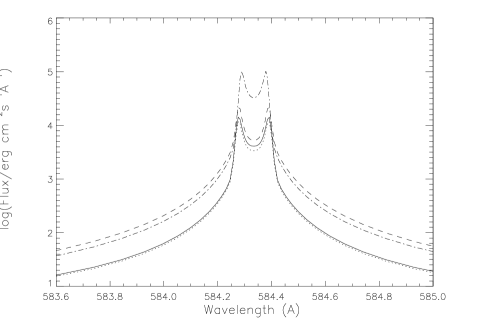
Figure 6: He i 584.3-Å line profiles produced by models VAL C (top), and network S (middle) and X (bottom), for non-Maxwellian EVDFs with $r_{\textrm{tail}}=3.5$ and $\xi_{\textrm{tail}}=5.0$ (solid), $\xi_{\textrm{tail}}=4.5$ (dotted), $\xi_{\textrm{tail}}=4.0$ (dashed), $\xi_{\textrm{tail}}=3.5$ (dot-dashed).

The somewhat surprising reduction of the 584.3-Å line intensity (compared to calculations with ‘normal’ Maxwellian rates) for higher $\xi_{\textrm{tail}}$ (compare Tables 4 and 2) appears to be due to a similar effect. The shift in the ionization balance suppresses the Maxwellian contribution to collisional excitation. The effect is smallest in model X, where Maxwellian collisional excitation is least significant because of the smaller amount of material in the relevant temperature range. The 584.3-Å line intensity can be reduced if the tail has a value of $\xi_{\textrm{tail}}$ too high for increased excitation by suprathermal electrons to compensate. Other lines of the He i resonance series do not show this, as the increased excitation has a greater effect than the shift in ionization (the suppressed Maxwellian contribution is relatively less significant).

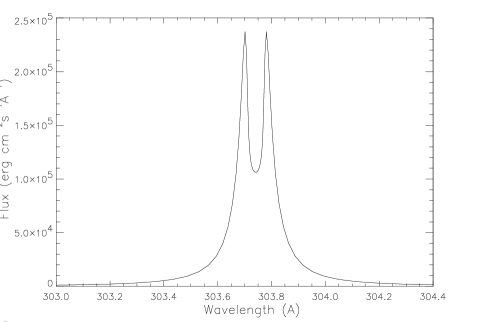
Figure 7: He ii 303.8-Å line profiles produced using network model S, with Maxwellian collision rates (top), and with a non-Maxwellian EVDF with $r_{\textrm{tail}}=3.5,\xi_{\textrm{tail}}=3.5$ (bottom).

The effect of enhanced ionization on the ionization balance also complicates the trend in the ratio $I$(537.0 Å)/$I$(584.3 Å), which is expected to decrease with decreasing $r_{\textrm{tail}}$. For low values of $\xi_{\textrm{tail}}$, the trend can reverse, as the change in the ionization balance affects the 584.3-Å line more than the 537.0-Å line, allowing $I$(537.0 Å) to grow more quickly with decreasing $\xi_{\textrm{tail}}$.

5.1 Comparison with observations

The results of the calculations may be compared with the mean line intensities observed by MJ99, which are given in Table 1. It can be seen that no particular combination of $\xi_{\textrm{tail}}$ and $r_{\textrm{tail}}$ leads to a good match to observations in all three lines for any of the model atmospheres tested.

In models in which the calculated 303.8-Å line intensity is comparable to observed values, the He i line ratio $I$(537.0 Å)/$I$(584.3 Å) is much larger than observed (independent of the cds calibration assumed), and the computed 303.8-Å line profile is in general self-reversed. Such reversals are not observed, but would probably not be resolved by the instruments on board SOHO [Smith 2000]. Models showing enhancements of the 303.8-Å line intensity comparing well with observations have other problems. The values of $\xi_{\textrm{tail}}$ required may be unrealistically low, but if such such a tail were present, significant collisional enhancement of the He ii 1640.4-Å multiplet is predicted. Intensities much larger than those observed, in some cases by orders of magnitude, are produced when $\xi_{\textrm{tail}}<4.5$ (independent of $r_{\textrm{tail}}$). This is in part due to the increased fraction of He ii at lower temperatures where recombination dominates the formation of the multiplet. Small departures from Maxwellian EVDFs might explain the Balmer $\alpha$ intensity, but results found here imply that non-Maxwellian collisional excitation could not be responsible for the observed resonance line intensity without producing too much Balmer $\alpha$ emission. It remains to be seen whether non-Maxwellian collisional excitation is consistent with observations of the profiles and relative intensities of the components of the 1640.4-Å multiplet. An improved treatment of the energy levels of He ii would allow an investigation of this point. The excitation of the 1640.4-Å multiplet by non-local electrons will also be tested against stellar observations in future work.

Trends in the results given in Tables 3 – 6 may be compared with observed variations in line intensities and ratios over different regions of the Sun. The effectiveness of the excitation mechanism depends on the temperature gradient and electron density, which have different values in the network and internetwork, in the quiet Sun and coronal holes. Given the significant disagreements between the calculations and observations described above, an approximate approach was followed in preference to constructing models of different parts of the atmosphere. The effects of different atmospheric parameters on the suprathermal electron tail are considered, and the results given in Tables 3 – 6 are used to infer how the helium line intensities might vary as a result.

Changes in the suprathermal tail may be parametrized in simple terms as variations of $\xi_{\textrm{tail}}$ and $r_{\textrm{tail}}$. The variation of $r_{\textrm{tail}}$ appears to depend on the energy balance in the atmosphere (Shoub 1982), and given the current lack of detailed understanding of the heating of the atmosphere, it is difficult to predict how conditions in different regions might affect $r_{\textrm{tail}}$. On the other hand, Shoub’s (1982) BGK calculations provide an expression for the variation of $\xi_{\textrm{tail}}$ with easily understood physical quantities:

$$\xi_{\textrm{tail}}\propto\left(\frac{T_{\textrm{h}}}{L}\right)^{-1/6}\left(\frac{N_{\textrm{e}}(T_{\textrm{h}})}{T_{\textrm{h}}}\right)^{1/6}\left(\frac{T}{T_{\textrm{h}}}\right)^{1/12}$$ (6)

where $L$ is the thickness of the transition region and $T_{\textrm{h}}$ is the temperature at its upper edge; $T_{\textrm{h}}/L$ corresponds to the average temperature gradient. $\xi_{\textrm{tail}}$ is therefore decreased (and the influence of the suprathermal tail increased) by an increase in $T_{\textrm{h}}$ or the temperature gradient d$T/$d$h$, or by a decrease in the electron pressure. This relation emerges from analytical calculations in a simplified system, but it shows expected dependences. The mean free path of an electron with a given velocity should increase with decreasing electron density, and the change in temperature over that path will increase as the temperature gradient steepens. Thus such changes increase the numbers of electrons from a region at $T_{1}$ reaching a region of lower temperature $T_{2}$. Increasing $T_{1}$ shifts the peak of the distribution function to higher energies, increasing the number of electrons in the tail with a given velocity. This also leads to an increase in the number of electrons with mean free paths large enough to influence lower temperature regions.

The dependence of $\xi_{\textrm{tail}}$ on each of the parameters is weak, but Tables 3 – 6 show that the helium line intensities can be sensitive to relatively small changes in $\xi_{\textrm{tail}}$. If changes in $\xi_{\textrm{tail}}$ are assumed to control the variation of helium line emission with position on the Sun, the predicted variations in intensities may be tested against observations.

With respect to average conditions in the quiet Sun, in coronal holes the electron pressure is 2 – 3 times smaller, the mean temperature gradient up to an order of magnitude smaller, and the coronal temperature at least 30 per cent smaller [Munro & Withbroe 1972, Jordan et al. 2001]. According to the expression in equation (6), $\xi_{\textrm{tail}}$ would then be a factor of up to $\sim 1.5$ larger in coronal holes than in the quiet Sun. Such a change spans the values investigated here; Tables 3 – 6 show that over such a range, very large changes in the helium line intensities can occur. The helium resonance line intensities are observed to be factors of 1.5 – 2.0 smaller in coronal holes than in the quiet Sun [Peter 1999, Jordan et al. 2001]. The present calculations suggest that such a decrease in He i line intensities would be accompanied by a large decrease in the $I$(537.0 Å)/$I$(584.3 Å) line ratio (perhaps by a factor of two or more). This would outweigh the small increase in the ratio expected with the reduction of coronal illumination. Observations [Jordan et al. 2001] suggest that the ratio is slightly larger in coronal holes than in the quiet Sun, contrary to the predictions of models dominated by non-Maxwellian collisional excitation. Changes in $\xi_{\textrm{tail}}$ of a factor of 1.5 also generally lead to significant variations in the calculated ratio of the He i and He ii resonance lines. In contrast, observations show no consistent variation in this ratio between coronal holes and the quiet Sun; the mean observed ratio is almost exactly the same in the two regions [Jordan et al. 2001].

The observed trends in line ratios in the quiet Sun may also be compared with the predictions of the calculations. In the quiet Sun MJ99 observed only small changes in the ratio $I$(537.0 Å)/$I$(584.3 Å) for changes in $I$(584.3 Å) of a factor of 5, the ratio decreasing with increasing $I$(584.3 Å). The ratio $I$(303.8 Å)/$I$(584.3 Å) is also observed to vary by relatively small amounts, and while consistent trends are not seen clearly, small values of the ratio often coincide with large values of $I$(584.3 Å). For large variations in $I$(584.3 Å), the calculations predict $I$(537.0 Å)/$I$(584.3 Å) to increase with increasing $I$(584.3 Å) in all but a small part of the parameter space, particularly for the (probably more realistic) smaller values of $r_{\textrm{tail}}$. The variation of the ratio is also larger than in observations. The predicted trend appears inevitable given the exciting mechanism, since the power law tail provides relatively greater numbers of electrons (with respect to a Maxwellian distribution) at the excitation energy of the 537.0-Å line than at the energy of the 584.3-Å line. The models also predict much larger variations in the ratio $I$(303.8 Å)/$I$(584.3 Å) than are observed for given changes in $I$(584.3 Å). Thus the predicted variations of the helium line ratios are not consistent with observations.

The comparisons made so far with quiet Sun observations have ignored the question of whether $\xi_{\textrm{tail}}$ would be expected to vary in a manner which would produce the observed variations in intensities between cell interior and network regions. In considering the dependence of $\xi_{\textrm{tail}}$ on the conditions in the quiet Sun transition region, the likely magnetic field geometry should be taken into account together with the changes in temperature gradient and electron pressure. All calculations described above assume any magnetic field to be aligned with a radial temperature gradient. In general, electrons streaming from the corona and upper TR would tend to follow the magnetic field, which in the lower TR and chromosphere is concentrated in the network. The model of Gabriel [Gabriel 1976] suggests that the temperature gradient in the direction of the magnetic field is largest in the centre of the network and decreases towards the edges. The model also predicted lower pressures in the network, while MJ99 observed such a trend. Both factors would cause $\xi_{\textrm{tail}}$ to be smallest at the centres of network boundaries, suggesting that enhancement of the helium line intensities by non-local electrons would be concentrated in the centre of the network. Such behaviour is not observed; indeed the helium network appears to be unusually broad (e.g. Brueckner & Bartoe 1974; Gallagher et al. 1998), and the enhancement of the helium lines with respect to other transition region lines appears to increase towards cell interiors (MJ99). This observed behaviour could be due to radiative transfer effects not considered in this simple argument, but it presents further problems for the proposed enhancement process. In contrast, it is argued in Paper I that enhancement by upward transport of helium ions in an expanding network field would lead naturally to the network appearing wider in the helium resonance lines than in other low TR lines.

5.2 Approximations in the EVDF

Given that the main approximation in the present work is that the form of the EVDF is assumed rather than calculated self-consistently, the extent to which the form chosen for the EVDF affects the computed line intensities should be considered. Two features of the EVDF in particular were investigated: the behaviour of the tail at very high velocities, and the dependence (or otherwise) of $\xi_{\textrm{tail}}$ on temperature.

Shoub’s [Shoub 1982] analytical results show a down-turn in the high energy tail, where the power law ceases to be a good description, at $\xi\sim 4.2\times 10^{3}T^{-1/2}$. The numerical calculations do not show this feature, these values of $\xi$ being outside the range of calculation, but it is plausible that such a down-turn should exist, as the above limit on $\xi$ decreases with increasing $T$, so that the EVDF tends towards the Maxwellian distribution assumed to exist in the near-isothermal corona. When calculations were made with a cut-off in the EVDF at the above $\xi(T)$, significant effects on the helium resonance lines were found for small $\xi_{\textrm{tail}}$. The decreased extent of the power law tail at higher temperatures reduces ionization rates from He i to He ii, decreasing the extent of the region where He ii dominates the ionization balance. Consequently, the intensity of the 303.8-Å line is decreased by up to a factor of 2, and the intensities of the He i lines are increased by up to 50 per cent. The cut-off is a crude device and calculations with $r_{\textrm{tail}}<3.5$ may well approximate the effects of the down-turn more accurately, but the sensitivity revealed here suggests that this part of the distribution may need closer attention in the future. The present results imply that including the down-turn properly in calculations would not improve the fit to observations.

The use in this study of EVDFs with $\xi_{\textrm{tail}}$ independent of $T$ is an approximation suggested by the general form of solutions to the Boltzmann equation. Shoub’s [Shoub 1982] analytical solutions suggest $\xi_{\textrm{tail}}\sim T^{1/12}$ (thus it changes by only 20 per cent for an order of magnitude change in $T$). Including such a dependence in calculations would be expected to worsen agreement with observations. The observed He ii resonance line intensity can only be produced by low values of $\xi_{\textrm{tail}}$, but the ratio of the 584.3-Å and 537.0-Å lines favours higher values, which would require $\xi_{\textrm{tail}}$ to vary with $T$ in the opposite sense. Ljepojevic & Burgess’ [Ljepojevic & Burgess 1990] results do show some increase in $\xi_{\textrm{tail}}$ for the lowest temperatures for which they present the EVDF. If $\xi_{\textrm{tail}}$ were lower at the higher $T$ of He ii line formation than at the lower $T$ of He i line formation, a better fit might be obtained, although the problem with the He ii Balmer $\alpha$ intensity would remain. This problem is certainly seen in the results of calculations made with enhanced collision rates operating only in He ii and not in He i, approximating very roughly the situation in which $\xi_{\textrm{tail}}$ is increased at low temperatures.

6 Summary and conclusions

A detailed study has been made of the formation of the helium resonance lines, involving radiative transfer calculations with a 36 level model helium atom. Calculations using the the VAL C (average quiet Sun) model atmosphere, with a coronal radiation field characteristic of the quiet Sun based on the solar irradiance model of Tobiska [Tobiska 1991], come close to reproducing the observed He i 584.3-Å line intensity, but produce intensities in the He i 537.0-Å and He ii 303.8-Å lines smaller than are observed. The predicted self-reversal of the 584.3-Å line is not observed, but it is shown that it may be largely obscured by instrumental effects. Calculations using the VAL D (network) model produce results in better agreement with observed network intensities, but the VAL models both produce poor matches to other transition region lines (e.g. of C ii and Si iii).

New model atmospheres (S and X) appropriate to network boundary regions were constructed to be more consistent with observed intensities of TR lines of species other than helium. Calculations using these new models with quiet coronal illumination fail to reproduce the observed quiet Sun network He ii resonance line intensity by factors of 7–8 (3–4 when the most recent cds calibration is used). Model X, based on the $\xi$ Boo A EMD, produces an intensity for the He i resonance line a factor of 7.5 smaller than observed, but model S, based on the MJ99 solar network EMD, gives better agreement. The computed intensity for the 584.3 Å line is a factor of 4 too small, but the computed line profile is closest to the observed one, having only a small self-reversal that could be completely obscured by instrumental broadening. The ratio $I$(537.0 Å)/$I$(584.3 Å) computed using model S also matches observations most closely.

The optical thickness of the He i and He ii resonance lines may explain the unusual width of the network observed in those lines if photons are scattered from the edges of the network. Studies of two-component model atmospheres are required to investigate this point.

In all of the model atmospheres the formation of the He ii resonance line is dominated by collisional excitation, but recombination is more important in the formation of the He ii 1640.4-Å multiplet. Recombination also contributes significantly to the intensity of the He i 584.3-Å line, but does not dominate its formation except in model X. Direct collisional excitation from the ground and indirect excitation by radiative transitions from other collisionally excited singlet levels also contribute significantly to the formation of the line. Similar formation processes are important in the He i 537.0-Å line.

Increasing the intensity of the coronal radiation field causes increases in the computed He i line intensities and generally produces a decrease in the $I$(537.0 Å)/$I$(584.3 Å) ratio. The He ii resonance line intensity is generally reduced by increased coronal illumination, as a shift in the peak He ii ionization fraction to lower temperatures reduces collisional excitation rates. Removing the coronal illumination produces very little change in the computed He ii resonance line intensity. An absence of coronal radiation does cause a reduction in the computed intensities of the He i lines, an effect approaching the observed reduction in model S, exceeding it in model X. The line ratio $I$(537.0 Å)/$I$(584.3 Å) is observed to be slightly larger in coronal holes than in the quiet Sun, and this feature is reproduced by the models with zero coronal illumination. The quite different responses to changes in coronal irradiance of the He i and He ii resonance lines suggest that this is not the factor controlling factor the intensities of both lines, given that they show similar behaviour, both in the quiet Sun and coronal holes, and that the ratio of their observed intensities does not change by large amounts (MJ99, Jordan et al. 2001).

Given that the intensities of the helium lines with respect to other TR lines are not explained by the ‘standard’ models used in the present work, modifications were made to the radiative transfer code to allow the effects of non-Maxwellian EVDFs on collision rates to be included in calculations of the helium line intensities. The EVDFs tested are of a form postulated to exist in the transition region because of the extreme temperature gradient (e.g. Shoub 1983); they are Maxwellian at thermal velocities, with a power law tail at suprathermal velocities. The parameters of the power law tail were varied in a range suggested by the results of Shoub (1982,1983) and Ljepojevic & Burgess [Ljepojevic & Burgess 1990], allowing an exploration of EVDFs that might plausibly be present in the model atmospheres studied here.

It is found that this simulation of the presence of an increased population of suprathermal electrons in the lower transition region can lead to significant enhancements of the helium resonance line intensities compared with models assuming Maxwellian electron distributions. None of the models tested, however, simultaneously reproduce the observed intensities of the three lines studied. Calculations in which the He ii resonance line intensity is approximately reproduced also produce a much larger intensity in the He ii 1640.4-Å multiplet than is observed. The enhanced collision rates produce large values of the He i line ratio $I$(537.0 Å)/$I$(584.3 Å), as the increase over Maxwellian rates is relatively greater in the higher energy transition. In some cases, where the power law tail is relatively insignificant, this produces better matches between the computed and observed ratios, but in cases where the suprathermal tail dominates excitation the computed ratio is generally much larger than observed. The calculations also predict that the ratio would increase with the absolute intensities of the lines, which is the opposite of the observed trend (MJ99).

A consideration of how local atmospheric conditions might affect the EVDF at a given temperature in the low TR suggests that a reduction of the helium resonance line intensities in coronal holes with respect to the quiet Sun would be expected if excitation by non-local electrons dominates line formation. However, the models also predict that a decrease in absolute He i intensities of the observed order would be accompanied by a decrease in the line ratio $I$(537.0 Å)/$I$(584.3 Å); the opposite is observed [Jordan et al. 2001]. This excitation process would also probably produce a larger variation in the ratio $I$(303.8 Å)/$I$(584.3 Å) than is observed between coronal holes and the quiet Sun [Jordan et al. 2001]. Similar considerations suggest that the appearance of the network in the helium lines is not easily explained in the case of excitation by non-local electrons.

In general, the calculations predict that significant departures from Maxwellian EVDFs of the form investigated would produce signatures in the helium line ratios which contradict observations. Small departures from Maxwellian EVDFs are not ruled out, but I conclude that collisional excitation by suprathermal electrons in EVDFs of the form examined here is unlikely to dominate the formation of the helium resonance lines. Enhancement by non-thermal transport of helium atoms and ions, as investigated in Paper I, appears to be a more promising explanation of the helium resonance line intensities.

The calculations performed in the present work contain a number of approximations, and the above conclusions are therefore contingent on a more sophisticated study of the excitation process. Ideally, such an investigation would be totally self-consistent, solving the Boltzmann equation for the EVDF and the equation of radiative transfer simultaneously. Models in which suprathermal electron populations are generated by reconnection events or MHD processes in the low TR (rather than by the steep TR temperature gradient) also deserve examination. The apparent sensitivity of the He ii 1640.4 Å multiplet to the presence of suprathermal electrons (in part through the altered ionization balance) suggests that these lines also deserve further investigation. In particular, the plausibility of enhanced suprathermal excitation could be tested against the observed profile of the multiplet and also against stellar observations.

Appendix

The new model atmospheres described in Section 2.2 are presented in the following pages. The tables give the logarithm (to base 10) of the mass column density $m$ (in units of g cm^-2), the electron temperature, the neutral hydrogen, proton, and electron number densities, the microturbulent velocity $v_{\textrm{\sc t}}$, and the height, $h$, above optical depth unity at 5000 Å.

Table 7: Network model S

log $m$	$T_{e}$ (K)	$N_{H}$ (cm-3)	$N_{p}$ (cm-3)	$N_{e}$ (cm-3)	$v_{\textrm{\sc t}}$ (km s-1)	$h$ (km)
-5.19127	1584853.9	5.145(+00)	3.474(+08)	4.168(+08)	24.997	1.07268(+04)
-5.17478	1413985.0	7.585(+00)	4.037(+08)	4.844(+08)	24.997	7.92048(+03)
-5.16217	1260642.6	1.112(+01)	4.652(+08)	5.582(+08)	24.997	6.00415(+03)
-5.15270	1124094.6	1.619(+01)	5.321(+08)	6.384(+08)	24.997	4.71803(+03)
-5.14560	1002513.0	2.347(+01)	6.049(+08)	7.258(+08)	24.997	3.85491(+03)
-5.14027	894411.1	3.388(+01)	6.845(+08)	8.214(+08)	24.997	3.27578(+03)
-5.13627	797921.2	4.885(+01)	7.721(+08)	9.263(+08)	24.997	2.88712(+03)
-5.13327	712247.2	7.026(+01)	8.679(+08)	1.041(+09)	24.997	2.62625(+03)
-5.13103	636407.8	1.008(+02)	9.727(+08)	1.167(+09)	24.997	2.45099(+03)
-5.12935	568948.6	1.444(+02)	1.088(+09)	1.305(+09)	24.997	2.33330(+03)
-5.12809	508595.4	2.073(+02)	1.215(+09)	1.457(+09)	24.997	2.25409(+03)
-5.12714	455771.6	2.957(+02)	1.352(+09)	1.622(+09)	24.997	2.20084(+03)
-5.12644	409125.0	4.206(+02)	1.500(+09)	1.800(+09)	24.997	2.16490(+03)
-5.12591	367575.5	5.980(+02)	1.661(+09)	1.993(+09)	24.997	2.14060(+03)
-5.12552	332266.8	8.359(+02)	1.828(+09)	2.193(+09)	24.997	2.12413(+03)
-5.12522	300036.4	1.176(+03)	2.011(+09)	2.413(+09)	24.997	2.11294(+03)
-5.12500	273347.0	1.612(+03)	2.194(+09)	2.632(+09)	24.997	2.10531(+03)
-5.12484	251069.5	2.155(+03)	2.373(+09)	2.847(+09)	24.997	2.10005(+03)
-5.12472	229606.0	2.935(+03)	2.575(+09)	3.089(+09)	24.997	2.09643(+03)
-5.12462	212574.0	3.843(+03)	2.761(+09)	3.313(+09)	24.994	2.09391(+03)
-5.12455	196161.2	5.111(+03)	2.971(+09)	3.565(+09)	24.882	2.09191(+03)
-5.12448	180448.0	6.928(+03)	3.216(+09)	3.859(+09)	24.348	2.09025(+03)
-5.12440	164226.6	9.827(+03)	3.518(+09)	4.221(+09)	23.738	2.08871(+03)
-5.12433	146786.9	1.504(+04)	3.913(+09)	4.696(+09)	23.017	2.08732(+03)
-5.12427	132660.1	2.230(+04)	4.308(+09)	5.169(+09)	22.366	2.08618(+03)
-5.12421	119174.1	3.423(+04)	4.769(+09)	5.722(+09)	21.679	2.08525(+03)
-5.12415	107764.9	5.180(+04)	5.247(+09)	6.296(+09)	21.034	2.08441(+03)
-5.12410	97241.1	8.011(+04)	5.785(+09)	6.941(+09)	20.378	2.08364(+03)
-5.12407	92216.0	1.010(+05)	6.086(+09)	7.302(+09)	20.018	2.08329(+03)
-5.12404	87313.9	1.287(+05)	6.411(+09)	7.692(+09)	19.667	2.08296(+03)
-5.12401	82287.5	1.682(+05)	6.781(+09)	8.136(+09)	19.307	2.08265(+03)
-5.12397	77765.1	2.186(+05)	7.160(+09)	8.591(+09)	18.908	2.08226(+03)
-5.12394	73242.7	2.904(+05)	7.584(+09)	9.100(+09)	18.510	2.08188(+03)
-5.12390	67996.6	4.167(+05)	8.141(+09)	9.768(+09)	18.047	2.08153(+03)
-5.12386	63590.1	5.824(+05)	8.674(+09)	1.041(+10)	17.658	2.08120(+03)
-5.12379	60973.2	7.230(+05)	9.035(+09)	1.084(+10)	17.368	2.08060(+03)
-5.12372	58494.9	8.985(+05)	9.406(+09)	1.129(+10)	17.093	2.08003(+03)
-5.12360	54142.5	1.362(+06)	1.018(+10)	1.216(+10)	16.610	2.07917(+03)
-5.12346	51072.7	1.884(+06)	1.072(+10)	1.287(+10)	16.234	2.07817(+03)
-5.12330	48242.2	2.612(+06)	1.133(+10)	1.360(+10)	15.868	2.07709(+03)
-5.12318	46212.0	3.362(+06)	1.182(+10)	1.418(+10)	15.605	2.07638(+03)
-5.12294	43432.6	4.893(+06)	1.256(+10)	1.507(+10)	15.196	2.07490(+03)
-5.12269	40763.2	7.276(+06)	1.337(+10)	1.604(+10)	14.802	2.07351(+03)
-5.12230	38241.0	1.101(+07)	1.424(+10)	1.709(+10)	14.382	2.07144(+03)
-5.12191	35751.7	1.733(+07)	1.522(+10)	1.827(+10)	13.966	2.06950(+03)
-5.12139	33983.7	2.479(+07)	1.602(+10)	1.923(+10)	13.629	2.06706(+03)
-5.12078	32054.2	3.810(+07)	1.702(+10)	2.043(+10)	13.201	2.06431(+03)
-5.12013	30042.2	6.235(+07)	1.819(+10)	2.184(+10)	12.742	2.06159(+03)
-5.11958	28359.9	9.789(+07)	1.929(+10)	2.315(+10)	12.358	2.05943(+03)
-5.11908	26829.4	1.529(+08)	2.041(+10)	2.445(+10)	12.008	2.05761(+03)
-5.11859	25301.5	2.480(+08)	2.171(+10)	2.576(+10)	11.660	2.05589(+03)
-5.11815	23939.0	3.962(+08)	2.314(+10)	2.677(+10)	11.348	2.05445(+03)
-5.11771	23198.1	5.173(+08)	2.407(+10)	2.734(+10)	11.111	2.05309(+03)
-5.11726	22448.8	6.803(+08)	2.502(+10)	2.800(+10)	10.872	2.05177(+03)
-5.11681	21697.9	8.973(+08)	2.593(+10)	2.880(+10)	10.631	2.05050(+03)
-5.11595	20262.9	1.527(+09)	2.762(+10)	3.059(+10)	10.173	2.04822(+03)
-5.11520	18997.3	2.422(+09)	2.912(+10)	3.230(+10)	9.768	2.04636(+03)
-5.11431	17510.5	4.057(+09)	3.088(+10)	3.440(+10)	9.292	2.04437(+03)
-5.11343	16023.6	6.535(+09)	3.263(+10)	3.656(+10)	8.817	2.04257(+03)
-5.11316	15474.6	7.641(+09)	3.314(+10)	3.723(+10)	8.749	2.04207(+03)
-5.11302	14826.2	8.934(+09)	3.372(+10)	3.799(+10)	8.744	2.04183(+03)

log $m$	$T_{e}$ (K)	$N_{H}$ (cm-3)	$N_{p}$ (cm-3)	$N_{e}$ (cm-3)	$v_{\textrm{\sc t}}$ (km s-1)	$h$ (km)
-5.11289	14231.2	1.021(+10)	3.428(+10)	3.872(+10)	8.741	2.04160(+03)
-5.11272	13448.8	1.201(+10)	3.508(+10)	3.973(+10)	8.736	2.04133(+03)
-5.11269	13316.1	1.234(+10)	3.523(+10)	3.994(+10)	8.735	2.04128(+03)
-5.11260	12860.5	1.348(+10)	3.574(+10)	4.059(+10)	8.733	2.04113(+03)
-5.11250	12467.5	1.454(+10)	3.621(+10)	4.113(+10)	8.731	2.04098(+03)
-5.11240	12012.6	1.582(+10)	3.682(+10)	4.174(+10)	8.728	2.04084(+03)
-5.11230	11555.1	1.718(+10)	3.759(+10)	4.220(+10)	8.725	2.04070(+03)
-5.11220	11097.5	1.861(+10)	3.862(+10)	4.233(+10)	8.723	2.04057(+03)
-5.11210	10813.9	1.958(+10)	3.937(+10)	4.220(+10)	8.720	2.04044(+03)
-5.11191	10700.7	2.016(+10)	3.959(+10)	4.203(+10)	8.719	2.04019(+03)
-5.11171	10599.0	2.071(+10)	3.978(+10)	4.188(+10)	8.718	2.03995(+03)
-5.11132	10405.0	2.176(+10)	4.012(+10)	4.164(+10)	8.717	2.03947(+03)
-5.11053	10007.5	2.393(+10)	4.075(+10)	4.142(+10)	8.713	2.03853(+03)
-5.10975	9610.0	2.620(+10)	4.123(+10)	4.151(+10)	8.710	2.03763(+03)
-5.10881	9529.3	2.727(+10)	4.107(+10)	4.131(+10)	8.702	2.03659(+03)
-5.10788	9450.1	2.830(+10)	4.093(+10)	4.114(+10)	8.694	2.03556(+03)
-5.10600	9288.7	3.029(+10)	4.072(+10)	4.088(+10)	8.678	2.03352(+03)
-5.10413	9128.8	3.225(+10)	4.054(+10)	4.068(+10)	8.661	2.03153(+03)
-5.10126	8883.4	3.522(+10)	4.034(+10)	4.046(+10)	8.637	2.02856(+03)
-5.09864	8658.3	3.793(+10)	4.022(+10)	4.032(+10)	8.614	2.02592(+03)
-5.09502	8480.8	4.077(+10)	3.996(+10)	4.006(+10)	8.593	2.02237(+03)
-5.08913	8365.4	4.402(+10)	3.949(+10)	3.960(+10)	8.571	2.01672(+03)
-5.08323	8250.0	4.721(+10)	3.912(+10)	3.922(+10)	8.550	2.01118(+03)
-5.07604	8125.0	5.094(+10)	3.872(+10)	3.883(+10)	8.525	2.00456(+03)
-5.06885	8000.0	5.468(+10)	3.839(+10)	3.850(+10)	8.500	1.99807(+03)
-5.05586	7870.0	6.057(+10)	3.787(+10)	3.799(+10)	8.460	1.98663(+03)
-5.04287	7740.0	6.649(+10)	3.749(+10)	3.762(+10)	8.420	1.97548(+03)
-5.02682	7635.0	7.371(+10)	3.729(+10)	3.742(+10)	8.320	1.96206(+03)
-5.01077	7530.0	8.108(+10)	3.726(+10)	3.739(+10)	8.220	1.94901(+03)
-4.98549	7420.3	9.204(+10)	3.745(+10)	3.760(+10)	8.099	1.92906(+03)
-4.96121	7322.3	1.031(+11)	3.787(+10)	3.804(+10)	7.976	1.91048(+03)
-4.93694	7247.5	1.147(+11)	3.850(+10)	3.867(+10)	7.834	1.89242(+03)
-4.88839	7116.9	1.399(+11)	4.006(+10)	4.026(+10)	7.577	1.85771(+03)
-4.82271	7005.8	1.773(+11)	4.242(+10)	4.265(+10)	7.323	1.81306(+03)
-4.76027	6900.2	2.207(+11)	4.477(+10)	4.503(+10)	7.081	1.77253(+03)
-4.66481	6786.4	3.030(+11)	4.839(+10)	4.871(+10)	6.733	1.71400(+03)
-4.55600	6698.4	4.275(+11)	5.215(+10)	5.260(+10)	6.357	1.65133(+03)
-4.43506	6600.7	6.211(+11)	5.566(+10)	5.618(+10)	5.938	1.58601(+03)
-4.30139	6535.7	9.185(+11)	5.898(+10)	5.970(+10)	5.523	1.51842(+03)
-4.15567	6475.9	1.385(+12)	6.294(+10)	6.392(+10)	5.096	1.44897(+03)
-4.07753	6443.9	1.718(+12)	6.524(+10)	6.640(+10)	4.877	1.41292(+03)
-3.99939	6411.8	2.125(+12)	6.812(+10)	6.950(+10)	4.659	1.37785(+03)
-3.91534	6380.7	2.661(+12)	7.222(+10)	7.387(+10)	4.432	1.34114(+03)
-3.83129	6355.5	3.320(+12)	7.739(+10)	7.937(+10)	4.219	1.30536(+03)
-3.65298	6256.8	5.324(+12)	8.481(+10)	8.769(+10)	3.777	1.23347(+03)
-3.47354	6127.5	8.547(+12)	8.741(+10)	9.159(+10)	3.356	1.16498(+03)
-3.30000	6135.4	1.313(+13)	1.125(+11)	1.187(+11)	2.960	1.10117(+03)
-3.13428	6112.0	1.982(+13)	1.356(+11)	1.445(+11)	2.592	1.04186(+03)
-2.97768	6044.7	2.936(+13)	1.489(+11)	1.612(+11)	2.262	9.87388(+02)
-2.83040	5955.0	4.258(+13)	1.539(+11)	1.702(+11)	1.961	9.37643(+02)
-2.68992	5851.9	6.071(+13)	1.520(+11)	1.729(+11)	1.689	8.91579(+02)
-2.55407	5736.4	8.529(+13)	1.433(+11)	1.690(+11)	1.538	8.48232(+02)
-2.42406	5589.2	1.187(+14)	1.230(+11)	1.527(+11)	1.416	8.07900(+02)
-2.29839	5444.7	1.635(+14)	1.027(+11)	1.365(+11)	1.299	7.70060(+02)
-2.17917	5291.1	2.222(+14)	8.018(+10)	1.175(+11)	1.193	7.35239(+02)
-2.07437	5132.7	2.923(+14)	5.753(+10)	9.920(+10)	1.108	7.05562(+02)
-2.02936	5061.5	3.291(+14)	4.829(+10)	9.219(+10)	1.073	6.93045(+02)

log $m$	$T_{e}$ (K)	$N_{H}$ (cm-3)	$N_{p}$ (cm-3)	$N_{e}$ (cm-3)	$v_{\textrm{\sc t}}$ (km s-1)	$h$ (km)
-1.98435	4987.5	3.708(+14)	3.945(+10)	8.598(+10)	1.041	6.80717(+02)
-1.90597	4858.6	4.566(+14)	2.616(+10)	7.875(+10)	0.985	6.59769(+02)
-1.83566	4746.6	5.502(+14)	1.718(+10)	7.715(+10)	0.937	6.41445(+02)
-1.77067	4646.6	6.534(+14)	1.120(+10)	7.977(+10)	0.894	6.24892(+02)
-1.70766	4549.5	7.723(+14)	7.059(+09)	8.551(+10)	0.851	6.09192(+02)
-1.64196	4469.2	9.155(+14)	4.747(+09)	9.481(+10)	0.809	5.93155(+02)
-1.56959	4402.8	1.099(+15)	3.421(+09)	1.076(+11)	0.763	5.75802(+02)
-1.48889	4328.7	1.348(+15)	2.345(+09)	1.231(+11)	0.713	5.56793(+02)
-1.39929	4297.7	1.670(+15)	2.089(+09)	1.450(+11)	0.669	5.35970(+02)
-1.30098	4280.3	2.105(+15)	2.023(+09)	1.741(+11)	0.626	5.13289(+02)
-1.18674	4277.6	2.742(+15)	2.147(+09)	2.167(+11)	0.582	4.87053(+02)
-1.05256	4295.8	3.722(+15)	2.574(+09)	2.837(+11)	0.540	4.56269(+02)
-0.90681	4354.9	5.137(+15)	3.845(+09)	3.911(+11)	0.527	4.22575(+02)
-0.76297	4423.9	7.043(+15)	5.907(+09)	5.405(+11)	0.524	3.88815(+02)
-0.62093	4492.0	9.620(+15)	8.866(+09)	7.427(+11)	0.520	3.54964(+02)
-0.48037	4586.4	1.302(+16)	1.511(+10)	1.034(+12)	0.555	3.20827(+02)
-0.34126	4683.4	1.755(+16)	2.612(+10)	1.434(+12)	0.593	2.86306(+02)
-0.20325	4782.3	2.359(+16)	4.641(+10)	1.981(+12)	0.637	2.51307(+02)
-0.06709	4930.9	3.122(+16)	1.088(+11)	2.798(+12)	0.774	2.15775(+02)
0.03467	5042.0	3.852(+16)	2.104(+11)	3.626(+12)	0.877	1.88360(+02)
0.11629	5131.1	4.559(+16)	3.582(+11)	4.480(+12)	0.959	1.65848(+02)
0.18791	5225.7	5.268(+16)	6.114(+11)	5.477(+12)	1.037	1.45685(+02)
0.25064	5327.2	5.959(+16)	1.043(+12)	6.671(+12)	1.111	1.27645(+02)
0.30637	5417.4	6.650(+16)	1.647(+12)	8.034(+12)	1.176	1.11293(+02)
0.35814	5527.4	7.330(+16)	2.721(+12)	9.911(+12)	1.240	9.57905(+01)
0.41162	5658.4	8.083(+16)	4.692(+12)	1.281(+13)	1.307	7.93916(+01)
0.46173	5781.2	8.863(+16)	7.524(+12)	1.659(+13)	1.370	6.36483(+01)
0.50584	5919.9	9.566(+16)	1.208(+13)	2.209(+13)	1.428	4.94471(+01)
0.54316	6068.0	1.016(+17)	1.897(+13)	2.987(+13)	1.479	3.71186(+01)
0.57682	6201.6	1.073(+17)	2.766(+13)	3.944(+13)	1.525	2.57236(+01)
0.61048	6335.2	1.133(+17)	3.936(+13)	5.205(+13)	1.571	1.40667(+01)
0.64141	6490.1	1.186(+17)	5.715(+13)	7.088(+13)	1.614	3.09627(+00)
0.65687	6603.4	1.208(+17)	7.334(+13)	8.765(+13)	1.637	-2.50818(+00)
0.67234	6716.7	1.229(+17)	9.314(+13)	1.081(+14)	1.661	-8.21229(+00)
0.69582	6888.8	1.264(+17)	1.315(+14)	1.475(+14)	1.696	-1.70655(+01)
0.70757	7011.2	1.275(+17)	1.651(+14)	1.817(+14)	1.709	-2.15903(+01)
0.71931	7145.4	1.285(+17)	2.095(+14)	2.269(+14)	1.720	-2.61991(+01)
0.73755	7353.9	1.301(+17)	2.977(+14)	3.164(+14)	1.738	-3.35360(+01)
0.75580	7562.4	1.318(+17)	4.146(+14)	4.346(+14)	1.756	-4.10870(+01)
0.77133	7754.9	1.330(+17)	5.52E(+14)	5.744(+14)	1.768	-4.76907(+01)
0.78686	7953.0	1.341(+17)	7.323(+14)	7.554(+14)	1.779	-5.44673(+01)
0.80107	8134.1	1.351(+17)	9.357(+14)	9.603(+14)	1.790	-6.08198(+01)
0.81517	8313.9	1.362(+17)	1.181(+15)	1.207(+15)	1.800	-6.72742(+01)

Table 8: Network model X

log $m$	$T_{e}$ (K)	$N_{H}$ (cm-3)	$N_{p}$ (cm-3)	$N_{e}$ (cm-3)	$v_{\textrm{\sc t}}$ (km s-1)	$h$ (km)
-5.19116	1584822.0	5.146(+00)	3.474(+08)	4.169(+08)	24.997	1.07156(+04)
-5.17478	1415053.0	7.568(+00)	4.034(+08)	4.840(+08)	24.997	7.92667(+03)
-5.16217	1261894.6	1.108(+01)	4.648(+08)	5.577(+08)	24.997	6.00867(+03)
-5.15270	1125551.6	1.613(+01)	5.314(+08)	6.376(+08)	24.997	4.72109(+03)
-5.14560	1004223.0	2.334(+01)	6.039(+08)	7.246(+08)	24.997	3.85669(+03)
-5.14027	896382.5	3.365(+01)	6.831(+08)	8.196(+08)	24.997	3.27644(+03)
-5.13627	800258.4	4.840(+01)	7.699(+08)	9.237(+08)	24.997	2.88681(+03)
-5.13327	715009.6	6.941(+01)	8.647(+08)	1.038(+09)	24.997	2.62507(+03)
-5.13103	639581.0	9.920(+01)	9.681(+08)	1.162(+09)	24.997	2.44905(+03)
-5.12935	572675.9	1.414(+02)	1.081(+09)	1.297(+09)	24.997	2.33070(+03)
-5.12809	513098.5	2.015(+02)	1.204(+09)	1.445(+09)	24.997	2.25091(+03)
-5.12714	461102.6	2.848(+02)	1.337(+09)	1.604(+09)	24.997	2.19713(+03)
-5.12644	415441.6	4.001(+02)	1.478(+09)	1.774(+09)	24.997	2.16072(+03)
-5.12591	375127.7	5.594(+02)	1.630(+09)	1.955(+09)	24.997	2.13602(+03)
-5.12552	341028.9	7.667(+02)	1.784(+09)	2.140(+09)	24.997	2.11918(+03)
-5.12522	310784.0	1.045(+03)	1.947(+09)	2.336(+09)	24.997	2.10766(+03)
-5.12500	285294.0	1.395(+03)	2.109(+09)	2.530(+09)	24.997	2.09975(+03)
-5.12484	263687.9	1.823(+03)	2.268(+09)	2.722(+09)	24.997	2.09426(+03)
-5.12472	244839.8	2.350(+03)	2.428(+09)	2.914(+09)	24.997	2.09044(+03)
-5.12462	229435.0	2.943(+03)	2.577(+09)	3.092(+09)	24.997	2.08776(+03)
-5.12455	214725.0	3.710(+03)	2.737(+09)	3.284(+09)	24.997	2.08561(+03)
-5.12448	201497.3	4.643(+03)	2.898(+09)	3.477(+09)	24.997	2.08378(+03)
-5.12440	185830.1	6.224(+03)	3.129(+09)	3.754(+09)	24.528	2.08206(+03)
-5.12433	168687.5	8.893(+03)	3.430(+09)	4.116(+09)	23.908	2.08048(+03)
-5.12427	153297.0	1.275(+04)	3.756(+09)	4.507(+09)	23.294	2.07918(+03)
-5.12421	137634.8	1.931(+04)	4.161(+09)	4.992(+09)	22.607	2.07812(+03)
-5.12415	123210.5	2.993(+04)	4.621(+09)	5.545(+09)	21.897	2.07716(+03)
-5.12410	109670.1	4.815(+04)	5.161(+09)	6.192(+09)	21.151	2.07628(+03)
-5.12407	102924.4	6.285(+04)	5.482(+09)	6.577(+09)	20.742	2.07590(+03)
-5.12404	96492.7	8.285(+04)	5.828(+09)	6.993(+09)	20.328	2.07554(+03)
-5.12401	89901.9	1.129(+05)	6.233(+09)	7.479(+09)	19.880	2.07520(+03)
-5.12397	83855.4	1.544(+05)	6.661(+09)	7.992(+09)	19.426	2.07477(+03)
-5.12394	78651.6	2.073(+05)	7.080(+09)	8.495(+09)	19.019	2.07437(+03)
-5.12390	73817.0	2.796(+05)	7.522(+09)	9.026(+09)	18.608	2.07399(+03)
-5.12386	70257.6	3.548(+05)	7.885(+09)	9.461(+09)	18.299	2.07363(+03)
-5.12379	65101.5	5.175(+05)	8.488(+09)	1.018(+10)	17.803	2.07298(+03)
-5.12372	61381.1	6.986(+05)	8.977(+09)	1.077(+10)	17.426	2.07238(+03)
-5.12362	56778.8	1.053(+06)	9.676(+09)	1.161(+10)	16.927	2.07164(+03)
-5.12354	53044.4	1.525(+06)	1.033(+10)	1.240(+10)	16.483	2.07104(+03)
-5.12346	49259.7	2.315(+06)	1.110(+10)	1.332(+10)	16.018	2.07048(+03)
-5.12338	45588.0	3.648(+06)	1.197(+10)	1.437(+10)	15.498	2.06997(+03)
-5.12330	41992.1	6.031(+06)	1.297(+10)	1.556(+10)	14.988	2.06949(+03)
-5.12321	38304.7	1.106(+07)	1.421(+10)	1.705(+10)	14.389	2.06904(+03)
-5.12312	34644.4	2.158(+07)	1.566(+10)	1.880(+10)	13.743	2.06860(+03)
-5.12306	32255.3	3.630(+07)	1.680(+10)	2.017(+10)	13.302	2.06832(+03)
-5.12300	29930.5	6.410(+07)	1.810(+10)	2.172(+10)	12.805	2.06806(+03)
-5.12294	27636.5	1.207(+08)	1.958(+10)	2.348(+10)	12.310	2.06783(+03)
-5.12288	25957.6	2.029(+08)	2.087(+10)	2.491(+10)	11.891	2.06761(+03)
-5.12282	24080.4	3.888(+08)	2.269(+10)	2.635(+10)	11.423	2.06740(+03)
-5.12275	22773.8	6.398(+08)	2.422(+10)	2.727(+10)	11.055	2.06722(+03)
-5.12269	21590.9	1.025(+09)	2.553(+10)	2.835(+10)	10.722	2.06704(+03)
-5.12260	19954.5	2.009(+09)	2.720(+10)	3.016(+10)	10.227	2.06678(+03)
-5.12250	19150.9	2.759(+09)	2.801(+10)	3.111(+10)	9.954	2.06654(+03)
-5.12230	17636.9	4.765(+09)	2.947(+10)	3.292(+10)	9.432	2.06610(+03)
-5.12211	17553.1	4.613(+09)	2.973(+10)	3.319(+10)	9.413	2.06569(+03)
-5.12191	17482.5	4.507(+09)	2.994(+10)	3.340(+10)	9.399	2.06527(+03)
-5.12165	17388.2	4.428(+09)	3.018(+10)	3.366(+10)	9.380	2.06472(+03)
-5.12139	17294.2	4.391(+09)	3.039(+10)	3.389(+10)	9.361	2.06417(+03)
-5.12078	17072.8	4.398(+09)	3.085(+10)	3.439(+10)	9.316	2.06287(+03)
-5.12013	16837.9	4.494(+09)	3.129(+10)	3.488(+10)	9.269	2.06151(+03)
-5.11958	16641.7	4.616(+09)	3.164(+10)	3.528(+10)	9.229	2.06039(+03)

log $m$	$T_{e}$ (K)	$N_{H}$ (cm-3)	$N_{p}$ (cm-3)	$N_{e}$ (cm-3)	$v_{\textrm{\sc t}}$ (km s-1)	$h$ (km)
-5.11908	16463.1	4.756(+09)	3.195(+10)	3.563(+10)	9.193	2.05939(+03)
-5.11815	16125.6	5.086(+09)	3.251(+10)	3.629(+10)	9.124	2.05752(+03)
-5.11726	15805.2	5.471(+09)	3.304(+10)	3.690(+10)	9.059	2.05579(+03)
-5.11595	15335.3	6.176(+09)	3.377(+10)	3.777(+10)	8.964	2.05331(+03)
-5.11431	14743.6	7.366(+09)	3.460(+10)	3.879(+10)	8.844	2.05032(+03)
-5.11316	14329.0	8.504(+09)	3.506(+10)	3.941(+10)	8.761	2.04830(+03)
-5.11302	14278.7	8.671(+09)	3.511(+10)	3.947(+10)	8.750	2.04807(+03)
-5.11289	14231.2	8.839(+09)	3.514(+10)	3.952(+10)	8.741	2.04784(+03)
-5.11272	13426.1	1.040(+10)	3.615(+10)	4.078(+10)	8.736	2.04756(+03)
-5.11269	13299.7	1.066(+10)	3.632(+10)	4.098(+10)	8.735	2.04751(+03)
-5.11260	12840.8	1.164(+10)	3.695(+10)	4.173(+10)	8.733	2.04736(+03)
-5.11250	12493.8	1.245(+10)	3.745(+10)	4.230(+10)	8.731	2.04721(+03)
-5.11240	12037.0	1.355(+10)	3.819(+10)	4.302(+10)	8.728	2.04706(+03)
-5.11230	11571.5	1.475(+10)	3.908(+10)	4.361(+10)	8.725	2.04693(+03)
-5.11220	11105.7	1.601(+10)	4.025(+10)	4.387(+10)	8.723	2.04679(+03)
-5.11210	10813.9	1.687(+10)	4.111(+10)	4.384(+10)	8.720	2.04666(+03)
-5.11191	10698.9	1.735(+10)	4.141(+10)	4.375(+10)	8.719	2.04641(+03)
-5.11171	10596.2	1.779(+10)	4.167(+10)	4.368(+10)	8.718	2.04616(+03)
-5.11132	10452.9	1.849(+10)	4.199(+10)	4.357(+10)	8.716	2.04567(+03)
-5.11053	10280.9	1.954(+10)	4.228(+10)	4.341(+10)	8.710	2.04470(+03)
-5.10975	10109.0	2.060(+10)	4.254(+10)	4.333(+10)	8.705	2.04375(+03)
-5.10881	9903.3	2.189(+10)	4.282(+10)	4.332(+10)	8.698	2.04264(+03)
-5.10788	9699.1	2.321(+10)	4.306(+10)	4.338(+10)	8.691	2.04156(+03)
-5.10600	9288.2	2.598(+10)	4.349(+10)	4.365(+10)	8.678	2.03946(+03)
-5.10413	9128.8	2.769(+10)	4.348(+10)	4.361(+10)	8.661	2.03742(+03)
-5.10126	8883.6	3.032(+10)	4.350(+10)	4.361(+10)	8.637	2.03438(+03)
-5.09864	8658.1	3.276(+10)	4.356(+10)	4.367(+10)	8.614	2.03168(+03)
-5.09502	8480.8	3.533(+10)	4.349(+10)	4.351(+10)	8.593	2.02804(+03)
-5.08913	8365.4	3.831(+10)	4.320(+10)	4.331(+10)	8.571	2.02225(+03)
-5.08323	8250.0	4.126(+10)	4.298(+10)	4.309(+10)	8.550	2.01657(+03)
-5.07604	8125.0	4.476(+10)	4.274(+10)	4.285(+10)	8.525	2.00979(+03)
-5.07245	8062.5	4.654(+10)	4.263(+10)	4.274(+10)	8.512	2.00645(+03)
-5.06885	8000.0	4.832(+10)	4.254(+10)	4.265(+10)	8.500	2.00314(+03)
-5.05586	7870.0	5.399(+10)	4.217(+10)	4.228(+10)	8.460	1.99143(+03)
-5.04287	7740.0	5.978(+10)	4.188(+10)	4.200(+10)	8.420	1.98002(+03)
-5.02682	7635.0	6.690(+10)	4.173(+10)	4.186(+10)	8.320	1.96630(+03)
-5.01077	7530.0	7.422(+10)	4.173(+10)	4.186(+10)	8.220	1.95298(+03)
-4.98543	7420.3	8.517(+10)	4.192(+10)	4.206(+10)	8.099	1.93263(+03)
-4.96121	7322.3	9.622(+10)	4.233(+10)	4.249(+10)	7.976	1.91371(+03)
-4.93694	7247.4	1.079(+11)	4.295(+10)	4.311(+10)	7.834	1.89535(+03)
-4.88839	7116.9	1.330(+11)	4.452(+10)	4.471(+10)	7.577	1.86012(+03)
-4.82271	7005.9	1.704(+11)	4.687(+10)	4.709(+10)	7.323	1.81490(+03)
-4.76027	6900.2	2.138(+11)	4.918(+10)	4.943(+10)	7.081	1.77394(+03)
-4.66481	6786.4	2.962(+11)	5.261(+10)	5.293(+10)	6.733	1.71493(+03)
-4.55600	6698.4	4.214(+11)	5.595(+10)	5.636(+10)	6.357	1.65188(+03)
-4.43506	6600.7	6.164(+11)	5.857(+10)	5.909(+10)	5.938	1.58639(+03)
-4.30139	6535.7	9.154(+11)	6.080(+10)	6.152(+10)	5.523	1.51861(+03)
-4.15567	6475.9	1.383(+12)	6.411(+10)	6.509(+10)	5.096	1.44911(+03)
-4.07753	6443.9	1.716(+12)	6.619(+10)	6.735(+10)	4.877	1.41303(+03)
-3.99939	6411.8	2.123(+12)	6.888(+10)	7.025(+10)	4.659	1.37795(+03)
-3.91534	6380.7	2.660(+12)	7.303(+10)	7.468(+10)	4.432	1.34124(+03)
-3.83129	6355.5	3.318(+12)	7.839(+10)	8.037(+10)	4.219	1.30545(+03)
-3.65298	6256.8	5.318(+12)	8.810(+10)	9.096(+10)	3.777	1.23355(+03)
-3.47354	6127.5	8.539(+12)	9.151(+10)	9.567(+10)	3.356	1.16501(+03)
-3.30000	6135.4	1.313(+13)	1.141(+11)	1.203(+11)	2.960	1.10119(+03)
-3.13428	6112.0	1.982(+13)	1.376(+11)	1.465(+11)	2.592	1.04187(+03)
-2.97768	6044.7	2.936(+13)	1.514(+11)	1.637(+11)	2.262	9.87399(+02)

log $m$	$T_{e}$ (K)	$N_{H}$ (cm-3)	$N_{p}$ (cm-3)	$N_{e}$ (cm-3)	$v_{\textrm{\sc t}}$ (km s-1)	$h$ (km)
-2.83040	5955.0	4.257(+13)	1.566(+11)	1.729(+11)	1.961	9.37651(+02)
-2.68992	5851.9	6.070(+13)	1.550(+11)	1.759(+11)	1.689	8.91585(+02)
-2.55407	5736.4	8.528(+13)	1.467(+11)	1.722(+11)	1.538	8.48236(+02)
-2.42406	5589.2	1.187(+14)	1.274(+11)	1.569(+11)	1.416	8.07902(+02)
-2.29839	5444.7	1.635(+14)	1.076(+11)	1.410(+11)	1.299	7.70062(+02)
-2.17917	5291.1	2.222(+14)	8.586(+10)	1.230(+11)	1.193	7.35240(+02)
-2.07437	5132.7	2.923(+14)	6.353(+10)	1.047(+11)	1.108	7.05562(+02)
-2.02936	5061.5	3.291(+14)	5.088(+10)	9.455(+10)	1.073	6.93045(+02)
-1.98435	4987.5	3.708(+14)	4.206(+10)	8.838(+10)	1.041	6.80717(+02)
-1.90597	4858.6	4.566(+14)	3.061(+10)	8.291(+10)	0.985	6.59768(+02)
-1.83566	4746.6	5.502(+14)	2.052(+10)	8.032(+10)	0.937	6.41444(+02)
-1.77067	4646.6	6.534(+14)	1.359(+10)	8.206(+10)	0.894	6.24891(+02)
-1.70766	4549.5	7.723(+14)	8.764(+09)	8.713(+10)	0.851	6.09191(+02)
-1.64196	4469.2	9.155(+14)	5.754(+09)	9.576(+10)	0.809	5.93154(+02)
-1.56959	4402.8	1.099(+15)	4.027(+09)	1.081(+11)	0.763	5.75801(+02)
-1.48889	4328.7	1.348(+15)	2.794(+09)	1.235(+11)	0.713	5.56793(+02)
-1.39929	4297.7	1.670(+15)	2.267(+09)	1.451(+11)	0.669	5.35970(+02)
-1.30098	4280.3	2.105(+15)	2.136(+09)	1.742(+11)	0.626	5.13289(+02)
-1.18674	4277.6	2.742(+15)	2.223(+09)	2.168(+11)	0.584	4.87053(+02)
-1.05256	4295.8	3.722(+15)	2.624(+09)	2.837(+11)	0.540	4.56269(+02)
-0.90681	4354.9	5.137(+15)	3.876(+09)	3.911(+11)	0.527	4.22570(+02)
-0.76297	4423.9	7.043(+15)	5.966(+09)	5.406(+11)	0.524	3.88814(+02)
-0.62093	4492.0	9.620(+15)	8.962(+09)	7.427(+11)	0.520	3.54964(+02)
-0.48037	4586.4	1.302(+16)	1.527(+10)	1.034(+12)	0.555	3.20827(+02)
-0.34126	4683.4	1.755(+16)	2.637(+10)	1.434(+12)	0.593	2.86306(+02)
-0.20325	4782.3	2.359(+16)	4.675(+10)	1.982(+12)	0.637	2.51306(+02)
-0.06709	4930.9	3.122(+16)	1.092(+11)	2.798(+12)	0.774	2.15774(+02)
0.03467	5042.0	3.852(+16)	2.108(+11)	3.626(+12)	0.877	1.88359(+02)
0.11629	5131.1	4.559(+16)	3.585(+11)	4.480(+12)	0.959	1.65848(+02)
0.18791	5225.7	5.268(+16)	6.116(+11)	5.477(+12)	1.037	1.45685(+02)
0.25064	5327.2	5.959(+16)	1.043(+12)	6.671(+12)	1.111	1.27645(+02)
0.30637	5417.4	6.650(+16)	1.647(+12)	8.035(+12)	1.176	1.11292(+02)
0.35814	5527.4	7.330(+16)	2.721(+12)	9.911(+12)	1.240	9.57900(+01)
0.41162	5658.4	8.083(+16)	4.692(+12)	1.281(+13)	1.307	7.93911(+01)
0.46173	5781.2	8.863(+16)	7.524(+12)	1.659(+13)	1.370	6.36477(+01)
0.50584	5919.9	9.566(+16)	1.208(+13)	2.209(+13)	1.428	4.94465(+01)
0.54316	6068.0	1.016(+17)	1.897(+13)	2.987(+13)	1.479	3.71181(+01)
0.57682	6201.6	1.073(+17)	2.766(+13)	3.944(+13)	1.525	2.57231(+01)
0.61048	6335.2	1.133(+17)	3.936(+13)	5.209(+13)	1.571	1.40661(+01)
0.64141	6490.1	1.186(+17)	5.715(+13)	7.088(+13)	1.614	3.09574(+00)
0.65687	6603.4	1.208(+17)	7.334(+13)	8.765(+13)	1.637	-2.5087(+00)
0.67234	6716.7	1.229(+17)	9.314(+13)	1.081(+14)	1.661	-8.21282(+00)
0.69582	6888.8	1.264(+17)	1.315(+14)	1.475(+14)	1.696	-1.70661(+01)
0.70757	7011.2	1.275(+17)	1.651(+14)	1.817(+14)	1.709	-2.15908(+01)
0.71931	7145.4	1.285(+17)	2.095(+14)	2.269(+14)	1.720	-2.61997(+01)
0.73755	7353.9	1.301(+17)	2.977(+14)	3.164(+14)	1.738	-3.35366(+01)
0.75580	7562.4	1.318(+17)	4.146(+14)	4.346(+14)	1.756	-4.10876(+01)
0.77133	7754.9	1.330(+17)	5.529(+14)	5.744(+14)	1.768	-4.76913(+01)
0.78686	7953.0	1.341(+17)	7.323(+14)	7.553(+14)	1.779	-5.44678(+01)
0.80107	8134.1	1.351(+17)	9.357(+14)	9.603(+14)	1.790	-6.08203(+01)
0.81517	8313.9	1.362(+17)	1.181(+15)	1.207(+15)	1.800	-6.72747(+01)

References

- [Aggarwal et al. 1991] Aggarwal K. M., Berrington K. A., Pathak A., 1991, J. Phys. B, 24, 1757
- [Aggarwal et al. 1992] Aggarwal K. M., Callaway J., Kingston A. E., Unnikrishnan K., 1992, ApJS, 80, 473
- [Anders & Grevesse 1989] Anders E., Grevesse N., 1989, Geochim. Cosmochim. Acta, 53, 197
- [Anderson 1994] Anderson S. W., 1994, ApJ, 437, 860
- [Anderson et al. 1996] Anderson S. W., Raymond J. C., Ballegooijen A. V., 1996, ApJ, 457, 939
- [Andretta & Jones 1997] Andretta V., Jones H. P., 1997, ApJ, 489, 375
- [Andretta et al. 2000] Andretta V., Jordan S. D., Brosius J. W., Davila J. M., Thomas R. J., Behring W. E., Thompson W. T., Garcia A., 2000, ApJ, 535, 438
- [Athay & Johnson 1960] Athay R. G., Johnson H. R., 1960, ApJ, 131, 413
- [Bashkin & Stoner 1975] Bashkin S., Stoner J. O., 1975, Atomic Energy Levels and Grotrian Diagrams, Volume I. North-Holland Publishing Co.
- [Bassani & Vignale 1982] Bassani F., Vignale G., 1982, Nuovo Cimento D, 1D, 519
- [Benson & Kulander 1972] Benson R. S., Kulander J. L., 1972, Solar Phys., 27, 305
- [Bhatnagar et al. 1954] Bhatnagar P. L., Gross E. P., Krook M., 1954, Phys. Rev., 94, 511
- [Bray et al. 1993] Bray I., McCarthy I. E., Wigley J., Stelbovics A. T., 1993, J. Phys. B, 26, L 831
- [Brekke et al. 2000] Brekke P., Thompson W. T., Woods T. N., Eparvier F. G., 2000, ApJ, 536, 959
- [Brueckner & Bartoe 1974] Brueckner G. E., Bartoe J-D. F., 1974, Solar Phys., 38, 133
- [Carlsson 1986] Carlsson M., 1986, Uppsala Astronomical Observatory, Report No. 33
- [Carlsson & Stein 1995] Carlsson M., Stein R. F., 1995, ApJ, 440, L 29
- [Cushman & Rense 1978] Cushman G. W., Rense W. A., 1978, Solar Phys., 58, 299
- [Deridder & Van Rensbergen 1976] Deridder G., Van Rensbergen W., 1976, A&AS, 23, 147
- [Dimitrijević & Sahal-Bréchot 1984] Dimitrijević M. S., Sahal-Bréchot S., 1984, JQSRT, 31, 301
- [Dimitrijević & Sahal-Bréchot 1990] Dimitrijević M. S., Sahal-Bréchot S., 1990, A&AS, 82, 519
- [Doschek et al. 1974] Doschek G. A., Behring W. E., Feldman U., 1974, ApJ, 190, L141
- [Drake 1996] Drake G. W. F., 1996, in Drake G. W. F., ed., Atomic, Molecular & Optical Physics Handbook. AIP Press, p. 154
- [Drake & Dalgarno 1969] Drake G. W. F., Dalgarno A., 1969, ApJ, 157, 459
- [Fernley et al. 1987] Fernley J. A., Taylor K. T., Seaton M. J., 1987, J. Phys. B, 20, 6457
- [Fontenla et al. 1993] Fontenla J. M., Avrett E. H., Loeser R., 1993, ApJ, 406, 319
- [Fontenla et al. 2002] Fontenla J. M., Avrett E. H., Loeser R., 2002, ApJ, 572, 636
- [Freudenstein & Cooper 1978] Freudenstein S. A., Cooper J., 1978, ApJ, 224, 1079
- [Gabriel 1976] Gabriel A. H., 1976, Phil. Trans. R. Soc. Lond., A 281, 339
- [Gallagher et al. 1998] Gallagher P. T., Phillips K. J. H., Harra-Murnion L. K., Keenan F. P., 1998, A&A, 335, 733
- [Green 1966] Green A. E. S., 1966, AAIA J., 4, 769
- [Grevesse et al. 1992] Grevesse N., Noels A., Sauval A. J., 1992, in Mattock C., ed., Proc. 1st SOHO Workshop, ESA SP-348, Coronal Streamers, Coronal Loops and Coronal and Solar Wind Composition. ESA Publications Division, Noordwijk, p. 305
- [Griem 1974] Griem H. G., 1974, Spectral Line Broadening by Plasmas. Academic Press
- [Hammer 1997] Hammer R., 1997, in Wilson A., ed., 5th SOHO Workshop, ESA SP-404, The Corona and Solar Wind Near Minimum Activity. ESA Publications Division, Noordwijk, p. 141
- [Hansteen et al. 1997] Hansteen V. H., Leer E., Holzer T. E., 1997, ApJ, 482, 498
- [Harper 1992] Harper G. M., 1992, MNRAS, 256, 37
- [Hearn 1969] Hearn A. G., 1969, MNRAS, 142, 53
- [Hinnov 1966] Hinnov E., 1966, J. Opt. Soc. Am., 56, 1179
- [Jordan 1975] Jordan C., 1975, MNRAS, 170, 429
- [Jordan 1980] Jordan C., 1980, Phil. Trans. R. Soc. Lond., A 297, 541
- [Jordan & Brown 1981] Jordan C., Brown A., 1981, in Bonnet R. M., Dupree A. K., eds, Solar Phenomena in Stars and Stellar Systems. Reidel, Dordrecht, p. 199
- [Jordan et al. 2001] Jordan C., Macpherson K. P., Smith G. R., 2001, MNRAS, 328, 1098
- [Kisielius et al. 1996] Kisielius R., Berrington K. A., Norrington P. H., 1996, A&AS, 118, 157
- [Kohl 1977] Kohl J. L., 1977, ApJ, 211, 958
- [Landau 1936] Landau L. D., 1936, Phys. Z. SowjUn., 10, 154. Translated in ter Haar D., ed., Collected Papers of L. D. Landau. Pergamon Press, p. 163
- [Landi et al. 1997] Landi E., Landini M., Pike C. D., Mason H. E., 1997, Solar Phys., 175, 553
- [Lanzafame et al. 1993] Lanzafame A. C., Tully J. A., Berrington K. A., Dufton P. L., Byrne P. B., Burgess A., 1993, MNRAS, 264, 402
- [Ljepojevic & Burgess 1990] Ljepojevic N. N., Burgess A., 1990, Proc. R. Soc., A 428, 71
- [Ljepojevic & MacNeice 1988] Ljepojevic N. N., MacNeice P., 1988, Solar Phys., 117, 123
- [Ljepojevic & MacNeice 1989] Ljepojevic N. N., MacNeice P., 1989, Phys. Rev. A, 40, 981
- [Macpherson & Jordan 1999] Macpherson K. P., Jordan C., 1999, MNRAS, 308, 510
- [McMurry 1997] McMurry A. D., 1997, DPhil thesis, University of Oxford
- [Martin 1987] Martin W. C., 1987, Phys. Rev. A, 36, 3575
- [Menzel & Pekeris 1935] Menzel D. H. and Pekeris C. L., 1935, MNRAS, 96, 77
- [Mihalas & Stone 1968] Mihalas D., Stone M. E., 1968, ApJ, 151, 293
- [Munro & Withbroe 1972] Munroe R. H., Withbroe G. L., 1972, ApJ, 176, 511
- [Peter 1999] Peter H., 1999, ApJ, 522, L77
- [Philippides 1996] Philippides D., 1996, DPhil Thesis, University of Oxford
- [Pinfield et al. 1999] Pinfield D. J., Keenan F. P., Mathioudakis M., Phillips K. J. H., Curdt W., Wilhelm K., 1999, ApJ, 527, 1000
- [Rowe 1996] Rowe A. K., 1996, DPhil thesis, University of Oxford
- [Sawey & Berrington 1993] Sawey P. M. J., Berrington K. A., 1993, A.D.N.D.T., 55, 81
- [Scharmer & Carlsson 1985] Scharmer G. B., Carlsson M., 1985, J. Comp. Phys., 59, 56
- [Scudder 1992a] Scudder J. D., 1992a, ApJ, 398, 299
- [Scudder 1992b] Scudder J. D., 1992b, ApJ, 398, 319
- [Scudder 1994] Scudder J. D., 1994, ApJ, 427, 446
- [Seaton 1987] Seaton M. J., 1987, J. Phys. B, 20, 6363
- [Shoub 1982] Shoub E. C., 1982, Stanford University Institute for Plasma Research, Report No. 946
- [Shoub 1983] Shoub E. C., 1983, ApJ, 266, 339
- [Smith 2000] Smith G. R., 2000, DPhil Thesis, University of Oxford
- [Smith & Jordan 2002] Smith G. R., Jordan C., 2002, MNRAS, 337, 666
- [Spitzer & Härm 1953] Spitzer L. and Härm R., 1953, Phys. Rev., 89, 977
- [Theodosiou 1987] Theodosiou C. E., 1987, A.D.N.D.T., 36, 97
- [Tobiska 1991] Tobiska W. K., 1991, J. Atmos. Terr. Phys., 53, 1005
- [Tobiska 1993] Tobiska W. K., 1993, J. Geophys. Res., 98, A11, 18879
- [Vernazza et al. 1981] Vernazza J. E., Avrett E. H., Loeser R., 1981, ApJS, 45, 635
- [Viñas et al. 2000] Viñas A. F., Wong H. K., Klimas A. J., 2000, ApJ, 528, 509
- [Wahlstrøm & Carlsson 1994] Wahlstrom C., Carlsson M., 1994, ApJ, 433, 417
- [Wiese et al. 1966] Wiese W. L., Smith M. W., Glennon B. M., 1966, Atomic Transition Probabilities, Volume I. N.S.R.D.S–N.B.S.4
- [Wilhelm et al. 1995] Wilhelm K. et al., 1995, Solar Phys., 162, 189