An integral equation approach to time-dependent kinematic dynamos in finite domains

Abstract

The homogeneous dynamo effect is at the root of cosmic magnetic field generation. With only a very few exceptions, the numerical treatment of homogeneous dynamos is carried out in the framework of the differential equation approach. The present paper tries to facilitate the use of integral equations in dynamo research. Apart from the pedagogical value to illustrate dynamo action within the well-known picture of Biot-Savart’s law, the integral equation approach has a number of practical advantages. The first advantage is its proven numerical robustness and stability. The second and perhaps most important advantage is its applicability to dynamos in arbitrary geometries. The third advantage is its intimate connection to inverse problems relevant not only for dynamos but also for technical applications of magnetohydrodynamics. The paper provides the first general formulation and application of the integral equation approach to time-dependent kinematic dynamos in finite domains. For the spherically symmetric $\alpha^{2}$ dynamo model it is shown how the general formulation is reduced to a coupled system of two radial integral equations for the defining scalars of the poloidal and the toroidal field components. The integral equation formulation for spherical dynamos with general velocity fields is also derived. Two numerical examples, the $\alpha^{2}$ dynamo model with radially varying $\alpha$, and the Bullard-Gellman model illustrate the equivalence of the approach with the usual differential equation method.

I Introduction

Cosmic magnetic fields, including the fields of planets, stars, and galaxies, result from the hydromagnetic dynamo effect KRRA ; MOFF . The last decades have seen tremendous progress in the analytical and numerical treatment of magnetic field generation in cosmic bodies. Recently, the hydromagnetic dynamo effect has been validated experimentally in large liquid sodium facilities in Riga and Karlsruhe PRL1 ; MUST ; PRL2 ; STMU ; RMP .

The usual way to treat hydromagnetic dynamos numerically is within the differential equation approach. Supposing the fluid velocity $\bf{u}$ to be given, the governing differential equation is the induction equation for the magnetic field $\bf{B}$,

$${}\frac{\partial{{\bf{B}}}}{\partial t}=\nabla\times({\bf{u}}\times{\bf{B}})+\frac{1}{\mu_{0}\sigma}\Delta{\bf{B}}\;,$$ (1)

with $\mu_{0}$ and $\sigma$ denoting the permeability of the free space and the electrical conductivity of the fluid, respectively. Equation (1) follows directly from pre-Maxwell’s equations and Ohm’s law in moving conductors. Note that the magnetic field has to be divergence-free:

$${}\nabla\cdot{\bf{B}}=0\;.$$ (2)

In case of vanishing excitations of the magnetic field from outside the considered finite region, the boundary condition for the magnetic field reads

$${}{\bf{B}}={\bf{O}}(r^{-3})\;\;\;\mbox{as}\;\;\;r\rightarrow\infty\;.$$ (3)

The induction equation (1) is sufficient to treat kinematic dynamo models in which the back-reaction of the self-excited magnetic field on the flow is neglected. Such a simplification is justified during the initial phase of self-excitation when the magnetic field is weak. For stronger fields, one has to cope with dynamically consistent dynamo models which require the simultaneous solution of the induction equation for the magnetic field and the Navier-Stokes equation for the velocity. This saturation regime, however, will not be considered in the present paper.

The spherical geometry of many cosmic bodies such as planets and stars has simplified dynamo simulations in one important respect: for the spherical case the boundary conditions for the magnetic field can be re-formulated separately for every degree and order of the spherical harmonics, which makes any particular treatment of the magnetic fields in the exterior superfluous.

When it comes to dynamos in other than spherical geometries, this pleasant situation changes. Then the correct handling of the non-local boundary conditions becomes non-trivial. Such a problem appears, e.g., in the numerical simulation of the recent dynamo experiments that are of cylindrical shape, but also in the simulations of galactic dynamos. There are some ways to circumvent this problem: one can use simplified local boundary conditions (“vertical field condition”) BRAN ; RUZH , one can embed the actual dynamo body into a sphere with the region between the actual dynamo and the surface of the sphere virtually filled with a medium of lower electrical conductivity RAE1 ; RAE2 , or one can solve the Laplace equation in the exterior and fit the solution at the boundary to the solution in the interior STE1 , which is, however, a tedious and time-consuming procedure.

The integral equation approach that we will establish in the present paper is intended to change this unsatisfactory situation concerning the handling of boundary conditions. For the steady case, and for infinite domains of homogeneous conductivity, the integral equation approach was used in a few previous papers GAI2 ; GAI3 ; FREI ; DORA . The inclusion of boundaries, again for the steady case, was already delineated in the book of Roberts ROB1 . In Roberts’ own opinion (ROB1 , p. 74), however, this formulation did “…not appear, in general, to be very useful.” In STE2 we have tried to put this pessimistic judgment into question. In particular, we have derived from the general theory a system of one-dimensional integral equations for a dynamo model with a spherically symmetric, isotropic helical turbulence parameter $\alpha$ in a finite sphere, and we have re-derived analytically the solution found by Krause and Steenbeck KRST for the special case of constant $\alpha$. In XUSG we have investigated the performance of numerical schemes to solve these integral equations for steady $\alpha^{2}$ dynamos.

It should be pointed out that a similar approach had been established earlier under the label “velocity-current-formulation” by Meir and Schmidt MES1 ; MES2 . This approach had also the pronounced aim to circumvent the numerical treatment outside the region of interest. However, the numerical focus of this work laid more on steady, coupled MHD problems with small magnetic Reynolds number than on dynamo problems.

In the present paper, we generalize the integral equation approach for steady dynamos in finite domains to the time-dependent case. In contrast to earlier statements on this matter DORA ; STE2 ; XUSG that the use of the Green’s function of the Helmholtz equation will lead us to a non-linear eigenvalue equation, we present here a linear formulation of the eigenvalue problem. This makes the approach more attractive for numerical treatment.

For the paradigmatic case of a time-dependent spherically symmetric, isotropic $\alpha^{2}$ dynamo we derive, starting from the general formulation, a coupled system of two radial integral equations which is solved numerically. The equivalence with the results of an differential equation solver is made evident.

We also derive the coupled system of radial integral equations for spherical dynamos with general velocity fields, and treat numerically the well-known Bullard-Gellman model within the new approach.

II General formulation

In this section, the general form of the integral equation approach is developed for time-dependent dynamos acting in an electrically conducting, non-magnetic fluid which occupies a finite domain $D$ with a boundary $S$, surrounded by non-conducting space. Under the assumption that the velocity or corresponding mean-field quantities are stationary, we generalize the basic idea and the methods from the steady case STE2 to the time-dependent case.

We start with pre-Maxwell’s equations (the displacement current can be skipped in the quasistationary approximation),

$${}\nabla\times{\bf{E}}({\bf{r}},t) = -\frac{\partial{\bf{B}}({\bf{r}},t)}{\partial t}\;,{}$$ (4)

$$\nabla\cdot{\bf{B}}({\bf{r}},t) = 0\;,{}$$ (5)

$$\nabla\times{\bf{B}}({\bf{r}},t) = \mu_{0}{\bf{j}}({\bf{r}},t)\;,{}$$ (6)

where ${\bf{B}}({\bf{r}},t)$ is the magnetic field, ${\bf{E}}({\bf{r}},t)$ the electric field, ${\bf{r}}$ the position vector, $t$ the time, and $\mu_{0}$ the magnetic permeability of the free space. The current density ${\bf{j}}({\bf{r}},t)$ satisfies Ohm’s law

$${}{\bf{j}}({\bf{r}},t)=\sigma({\bf{E}}({\bf{r}},t)+{\bf{F}}({\bf{r}},t))$$ (7)

inside the dynamo domain $D$, and it vanishes outside $D$. ${\bf{F}}({\bf{r}},t)$ denotes the electromotive force (emf) ${\bf{u}}({\bf{r}})\times{\bf{B}}({\bf{r}},t)$, where ${\bf{u}}({\bf{r}})$ is the velocity of the fluid motion, which we suppose to be stationary. In the framework of mean-field electrodynamics (see, e.g., KRRA ) ${\bf{B}}({\bf{r}},t)$, ${\bf{j}}({\bf{r}},t)$ and ${\bf{F}}({\bf{r}},t)$ are split into mean fields and fluctuating fields. Then ${\bf{F}}({\bf{r}},t)$ can be fixed to the form

$${}{\bf{F}}({\bf{r}},t)={\bf{u}}({\bf{r}})\times{\bf{B}}({\bf{r}},t)+\alpha({\bf{r}}){\bf{B}}({\bf{r}},t)-\beta({\bf{r}})\nabla\times{\bf{B}}({\bf{r}},t),$$ (8)

where ${\bf{u}}({\bf{r}})$ and ${\bf{B}}({\bf{r}},t)$ now denote the mean velocity and the mean magnetic field, respectively. The term $\alpha({\bf{r}})\bf{B}({\bf{r}},t)$ describes the emf due to the non-mirrorsymmetric part of the turbulence ($\alpha$-effect), and the term $\beta({\bf{r}})\nabla\times{\bf{B}}({\bf{r}},t)$ describes another effect which can be interpreted as an conductivity decrease due to the turbulence ($\beta$-effect).

The equations given so far, together with initial conditions for ${\bf{B}}$, define an initial value problem for ${\bf{B}}({\bf{r}},t)$ which can be combined into the form of Eq. (1). Together with the requirements that there are no surface currents on $S$ and that ${\bf{B}}({\bf{r}},t)$ vanishes at infinity, they allow to determine ${\bf{B}}({\bf{r}},t)$ once the concrete dependence of ${\bf{F}}({\bf{r}},t)$ on ${\bf{B}}({\bf{r}},t)$ has been fixed.

Under the condition that $\bf{u}$, $\alpha$ and $\beta$ in Eq. (8) only depend on the position ${\bf{r}}$, the functions ${\bf{E}}({\bf{r}},t)$, ${\bf{B}}({\bf{r}},t)$, ${\bf{F}}({\bf{r}},t)$ and ${\bf{j}}({\bf{r}},t)$ may be written in the form:

$${}{\bf{E}}({\bf{r}},t)={\bf{E}}({\bf{r}})e^{\lambda t},\;{\bf{B}}({\bf{r}},t)={\bf{B}}({\bf{r}})e^{\lambda t},\;{\bf{F}}({\bf{r}},t)={\bf{F}}({\bf{r}})e^{\lambda t},\;{\bf{j}}({\bf{r}},t)={\bf{j}}({\bf{r}})e^{\lambda t},$$ (9)

where $\lambda$ is in general a complex constant. Then Maxwell’s equations and Ohm’s law transform into

$$\nabla\times{\bf{E}} = -\lambda{\bf{B}}\;,{}$$ (10)

$$\nabla\cdot{\bf{B}} = 0\;,{}$$ (11)

$$\nabla\times{\bf{B}} = \mu_{0}{\bf{j}}{}\;,$$ (12)

$${\bf{j}} = \sigma({\bf{E}}+{\bf{F}})\;.{}$$ (13)

Hereafter, the symbols ${\bf{B}}$, ${\bf{E}}$, ${\bf{j}}$ and ${\bf{F}}$ denote the functions which only depend on the position ${\bf{r}}$, but not on the time $t$.

Since the magnetic field $\bf{B}$ is divergence-free, there exists a magnetic vector potential ${\bf{A}}({\bf{r}})$ such that

$${}{\bf{B}}=\nabla\times{\bf{A}},$$ (14)

which implies, together with Eq. (10), that

$${}\nabla\times({\bf{E}}+\lambda{\bf{A}})=0\;.$$ (15)

Therefore, ${\bf{E}}+\lambda{\bf{A}}$ has to be irrotational, and we can write

$${}{\bf{E}}+\lambda{\bf{A}}=-\nabla\varphi\;.$$ (16)

Subsequently, Ohm’s law gets the form

$${}{\bf{j}}=\sigma({\bf{F}}-\lambda{\bf{A}}-\nabla\varphi).$$ (17)

In the following, we will derive a system of integral equations that is equivalent to the differential equation formulation. The starting point for the first integral equation is the application of Biot-Savart’s law on Eq. (12), leading to

$${}{\bf{B}}({\bf{r}}) = \frac{\mu_{0}}{4\pi}\int_{D}\frac{{\bf{j}}({\bf{r^{\prime}}})\times({\bf{r}}-{\bf{r^{\prime}}})}{|{\bf{r}}-{\bf{r^{\prime}}}|^{3}}\;dV^{\prime}\;.$$ (18)

It is well known that the $curl$ operator in Eq. (12) is a left inverse of the Biot-Savart operator when the current $\bf j$ is divergence-free and tangent to the boundary of the domain CANT . Both conditions are indeed fulfilled in our case. Inserting Eq. (17) into Eq. (18), using Eq. (14) and Gauss’s theorem, we get the first integral equation

$${}{\bf{B}}({\bf{r}}) = \frac{\mu_{0}\sigma}{4\pi}\int_{D}\frac{{\bf{F}}({\bf{r^{\prime}}})\times({\bf{r}}-{\bf{r^{\prime}}})}{|{\bf{r}}-{\bf{r^{\prime}}}|^{3}}\;dV^{\prime}-\frac{\mu_{0}\sigma\lambda}{4\pi}\int_{D}\frac{{\bf{B}}({\bf{r^{\prime}}})}{|{\bf{r}}-{\bf{r^{\prime}}}|}\;dV^{\prime}$$ (19)

$$+\frac{\mu_{0}\sigma\lambda}{4\pi}\int_{S}{\bf{n}}({\bf{s^{\prime}}})\times\frac{{\bf{A}}({\bf{s^{\prime}}})}{|{\bf{r}}-{\bf{s^{\prime}}}|}\;dS^{\prime}-\frac{\mu_{0}\sigma}{4\pi}\int_{S}\varphi({\bf{s^{\prime}}}){\bf{n}}({\bf{s^{\prime}}})\times\frac{{\bf{r}}-{\bf{s^{\prime}}}}{|{\bf{r}}-{\bf{s^{\prime}}}|^{3}}\;dS^{\prime},$$

with ${\bf{n}}({\bf{s^{\prime}}})$ denoting the outward directed unit vector at the boundary point $\bf{s^{\prime}}$ and $dS^{\prime}$ denoting an area element at this point. For some purposes it might be useful to express the first volume integral in Eq. (19) in the form

$$\int_{D}\frac{{\bf{F}}({\bf{r^{\prime}}})\times({\bf{r}}-{\bf{r^{\prime}}})}{|{\bf{r}}-{\bf{r^{\prime}}}|^{3}}\;dV^{\prime} = \int_{D}\frac{\nabla_{r^{\prime}}\times{\bf{F}}({\bf{r^{\prime}}})}{|{\bf{r}}-{\bf{r^{\prime}}}|}\;dV^{\prime}-\int_{S}{\bf{n}}({\bf{s^{\prime}}})\times\frac{{\bf{F}}({\bf{s^{\prime}}})}{|{\bf{r}}-{\bf{s^{\prime}}}|}\;dS^{\prime}\;.$$ (20)

For the steady case ($\lambda=0$) Eq. (19) reduces to the form given in STE2 , with one volume integral over $\bf{B}$ and one boundary integral over $\varphi$. The latter one would vanish only in the case that the dynamo region is extended to infinity. The time-dependence introduces now a new volume integral over $\bf{B}$, but also one boundary integral over the vector potential $\bf{A}$ which cannot be reduced to a simple expression in $\bf{B}$. Before we focus on this point, let us first derive the integral equation for $\varphi$.

From Eq. (17) and the demand that the current has to be divergence-free, $\nabla\cdot{\bf{j}}=0$, we get a Poisson equation for $\varphi$:

$${}\Delta\varphi=\nabla\cdot({\bf F}-\lambda{\bf A})\;.$$ (21)

Assuming vacuum boundary condition which means that the current must not leave the domain $D$, we obtain from Green’s theorem the following boundary integral equation for $\varphi$:

$${}p\;\varphi({\bf{r}}) = \frac{1}{4\pi}\int\limits_{D}\frac{{\bf{F}}({\bf{r^{\prime}}})\cdot({\bf{r}}-{\bf{r^{\prime}}})}{|{\bf{r}}-{\bf{r^{\prime}}}|^{3}}\;dV^{\prime}+\frac{\lambda}{4\pi}\int\limits_{D}\frac{\nabla_{r^{\prime}}\cdot{\bf A}({\bf{r^{\prime}}})}{|{\bf{r}}-{\bf{r^{\prime}}}|}\;dV^{\prime}$$ (22)

$$-\frac{\lambda}{4\pi}\int\limits_{S}{\bf{n}}({\bf{s^{\prime}}})\cdot\frac{{\bf{A}}({\bf{s^{\prime}}})}{|{\bf{r}}-{\bf{s^{\prime}}}|}\;dS^{\prime}-\frac{1}{4\pi}\int\limits_{S}\varphi({\bf{s^{\prime}}}){\bf{n}}({\bf{s^{\prime}}})\cdot\frac{{\bf{r}}-{\bf{s^{\prime}}}}{{|{\bf{r}}-{\bf{s^{\prime}}}|}^{3}}\;dS^{\prime},$$

where $p=1$ for points $\bf{r}$ inside $D$, $p=1/2$ for points ${\bf{r}}={\bf{s}}$ on $S$ and $p=0$ for points $\bf{r}$ outside $D$. Again, another expression of the first volume integral might be useful :

$$\int_{D}\frac{{\bf{F}}({\bf{r^{\prime}}})\cdot({\bf{r}}-{\bf{r^{\prime}}})}{|{\bf{r}}-{\bf{r^{\prime}}}|^{3}}\;dV^{\prime} = -\int_{D}\frac{\nabla\cdot{\bf{F}}({\bf{r^{\prime}}})}{|{\bf{r}}-{\bf{r^{\prime}}}|}\;dV^{\prime}+\int_{S}{\bf{n}}({\bf{s^{\prime}}})\cdot\frac{{\bf{F}}({\bf{s^{\prime}}})}{|{\bf{r}}-{\bf{s^{\prime}}}|}\;dS^{\prime}\;.$$ (23)

If we use the Coulomb gauge for the vector potential, $\nabla\cdot{\bf{A}}=0$, we see that the second volume integral in Eq. (22) vanishes. Of course, one is free to use other gauges than the Coulomb gauge. One advantage of this gauge, in view of later numerical applications, is that it leads to a formulation in which the vector potential is only needed at the boundary of the domain.

For the steady case, Eqs. (19) and (22) with $\lambda=0$ are sufficient to determine the magnetic field $\bf{B}$. But for the time-dependent case presently under consideration, we have to introduce the vector potential $\bf{A}$, at least at the boundary, for completely formulating the problem. Necessarily we have to establish another relation for $\bf{A}$ in order to make the problem solvable. From Eq. (14) and Helmholtz’s theorem (MORS , p. 53) we can express the vector potential at the boundary in one of the two forms

$${}{\bf{A}}({\bf{s}}) = \frac{1}{4\pi}\int_{D}\frac{\nabla_{r^{\prime}}\times{\bf{B}}({\bf{r}}^{\prime})}{|{\bf{r}}-{\bf{r}}^{\prime}|}dV^{\prime}$$ (24)

$$= \frac{1}{4\pi}\int_{D}\frac{{\bf{B}}({\bf{r^{\prime}}})\times({\bf{s}}-{\bf{r^{\prime}}})}{|{\bf{s}}-{\bf{r^{\prime}}}|^{3}}dV^{\prime}+\frac{1}{4\pi}\int_{S}{\bf{n}}({\bf{s^{\prime}}})\times\frac{{\bf{B}}({\bf{s^{\prime}}})}{|{\bf{s}}-{\bf{s^{\prime}}}|}dS^{\prime}\;.$$

The integral equations (19), (22) and (24) provide another complete formulation of the problem for $\bf{B}$. The main advantage of this formulation is that one can avoid any treatment of fields in the exteriour of $D$. The boundary conditions are being fulfilled by solving the boundary integral equations for $\varphi$ and $\bf{A}$.

In the next section we will sketch how the equations for $\bf{A}$ and $\varphi$ at the boundary can be absorbed into a single integral equation for $\bf{B}$.

III General numerical aspects

In this section we delineate the general framework for the numerical solution of the coupled equations (19), (22) and (24). Let us assume certain spatial discretizations of the magnetic field in the volume of the dynamo, and of the electric potential and the vector potential at the boundary. Then, Eq. (19) may be rewritten in the form

$${}B_{i}=L_{ik}B_{k}+\lambda M_{ik}B_{k}+\lambda P_{in}A_{n}+N_{il}\varphi_{l}\;,$$ (25)

where the $B_{i}$ denote the degrees of freedom of the magnetic field in the volume of the dynamo, while $\varphi_{l}$ and $A_{n}$ denote the degrees of freedom of the electric potential and the vector potential at the boundary. Here and in the following we use Einstein’s summation convention, and we reserve the indices $i,k$ for magnetic field degrees of freedom in the volume of the fluid, whereas the indices $l,m,n$ are reserved for the vector potential and electric potential degrees of freedom at the boundary of the fluid.

For any given dynamo source, any shape of the dynamo domain, and any concrete form of the discretization, the matrices ${\bf{L}}$, ${\bf{M}}$, ${\bf{N}}$ and ${\bf{P}}$ in Eq. (25) can easily be derived from Eq. (19). It is worthwhile to note that only ${\bf{L}}$ depends on the dynamo source (${\bf{u}}$ or $\alpha$), whereas ${\bf{M}}$, ${\bf{N}}$ and ${\bf{P}}$ depend only on the geometry of the dynamo domain and the discretization details.

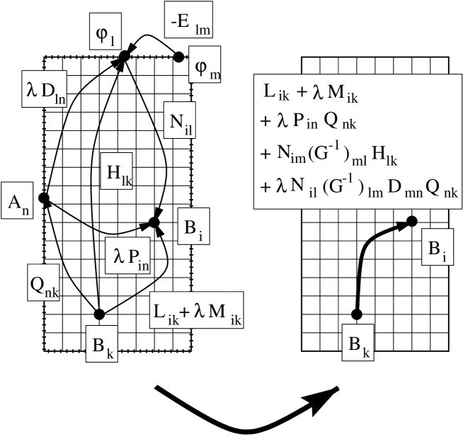
Figure 1: The general scheme for the numerical realization of the integral equation approach. Left: The connection between the magnetic fields in the volume and the vector potential and the electric potential on the boundary. Right: Reduction to the pure connection between magnetic fields in the volume. The boundary on the l.h.s. is indicated to have a finer discretization then the volume. On the r.h.s. the influence of the boundary has been incorporated implicitly. For details, cp the formulae in the text.

Similarly, the discretization of the boundary integral equation (22) (for the case that ${\bf{r}}$ is on the surface $S$) leads to

$${}0.5\;\varphi_{l}+E_{lm}\varphi_{m}=H_{lk}B_{k}+\lambda D_{ln}A_{n},$$ (26)

or

$${}G_{lm}\varphi_{m}=H_{lk}B_{k}+\lambda D_{ln}A_{n},$$ (27)

where $G_{lm}=0.5\;\delta_{lm}+E_{lm}$. Again one should note that only ${\bf{H}}$ depends on the dynamo source, whereas ${\bf{G}}$ and ${\bf{D}}$ depend only on the geometry of the dynamo domain and the discretization details. The discretization of Eq. (24) gives

$${}A_{n}=Q_{nk}B_{k}\;,$$ (28)

with $\bf Q$ depending solely on the geometry. The influence of the magnetic field degrees of freedom on the vector potential and the electric potential degrees of freedom on the boundary, and vice versa, is illustrated on the l.h.s. of Fig. 1.

Substituting Eq. (28) into Eq. (27) yields

$${}\varphi_{m}=(G^{-1})_{ml}H_{lk}B_{k}+\lambda(G^{-1})_{ml}D_{ln}Q_{nk}B_{k}.$$ (29)

However, for the inversion of the matrix $\bf G$ some care is needed. Basically, $\bf G$ is a singular matrix, reflecting the fact that the electric potential is determined only up to a constant. Accidently, it may happen that this singularity is weakened by inaccuracies due to the discretization. Nevertheless, one should be careful with the inversion. A convenient method to deal with the inversion is the application of the deflation method BARN ; SARV . In the following, we will simply assume that the inverse of $\bf G$ has been found in an appropriate manner.

After inserting Eqs. (28) and (29), Eq. (25) is transformed to

$${}B_{i}=L_{ik}B_{k}+\lambda M_{ik}B_{k}+\lambda P_{in}Q_{nk}B_{k}+N_{im}(G^{-1})_{ml}H_{lk}B_{k}+\lambda N_{il}(G^{-1})_{lm}D_{mn}Q_{nk}B_{k}.$$ (30)

Evidently, the electric potential and the magnetic vector potential at the boundary served only as auxiliary quantities in order to ensure the right boundary conditions. From the numerical viewpoint it is important to take notice of the following: for the accurate solution of the boundary integral equation (29) for a dynamo in a given domain it may be advisable to use a fine discretization of the boundary with a large number of grid points. Hence, the corresponding inversion of the matrix $\bf G$ might be numerically expensive. However, for a given geometry this inversion is needed only once. Finally, after carrying out the matrix multiplications $\bf N\cdot G^{-1}\cdot H$ and $\bf N\cdot G^{-1}\cdot D\cdot Q$ in Eq. (30) one ends up with a matrix of the order $(NB,NB)$ where $NB$ denotes the total number of all magnetic field degrees of freedom (see the r.h.s. of Fig. (1)).

Now, Eq. (30) can be rewritten in the following form:

$${}(\delta_{ik}-L_{ik}-N_{im}(G^{-1})_{ml}H_{lk})B_{k}=\lambda(M_{ik}+P_{in}Q_{nk}+N_{il}(G^{-1})_{lm}D_{mn}Q_{nk})B_{k}.$$ (31)

This is a generalized linear matrix eigenvalue problem in which only the magnetic field components remain. The numerical solution of the arising linear generalized eigenvalue equation (31) yields the eigenvalues $\lambda$, comprising as the real part the growth rate and as the imaginary part the frequency of the dynamo.

IV Application to time-dependent $\alpha^{2}$ dynamos - Basics

In this section, we exemplify the general integral equation approach by applying it to a simple mean-field dynamo model with a spherically symmetric, isotropic helical turbulence parameter $\alpha$. In contrast to the original model with constant $\alpha$ KRST ; KRRA , whose advantage is the possibility of an analytical treatment, we allow here $\alpha$ to vary with the radial coordinate $r$. Starting from equations (19), (22) and (24) we will derive two coupled radial integral equations which will be used in the next section for numerical treatment. Note that for the steady case the corresponding derivation had been given in STE2 .

Basically, this section is intended as an exercise to show how the basic integral equation approach can be reduced in a particular case with high symmetry of the dynamo source. A slightly simpler derivation of the two radial integral equations, which starts from the radial differential equations and uses a Green’s function method, is given in Appendix A. If the reader is only interested in the final form of the radial integral equations he can skip the following derivations and refer directly to Eqs. (47) and (67).

IV.1 Preliminaries

As usual in dynamo theory, we split the divergence-free magnetic field $\bf{B}$ into a poloidal and a toroidal part, denoted by ${\bf{B}}_{P}$ and ${\bf{B}}_{T}$. Since we use the Coulomb gauge, $\nabla\cdot{\bf A}=0$, an equivalent decomposition can also be applied to the vector potential, ${\bf A}={\bf{A}}_{P}+{\bf{A}}_{T}$. We represent these fields by the defining scalars $S$, $T$, $S^{A}$, $T^{A}$ according to

$${}{\bf{B}}_{P}=\nabla\times\nabla\times\left(\frac{S}{r}\,{\bf{r}}\right),\;\;\;{\bf{B}}_{T}=\nabla\times\left(\frac{T}{r}\,{\bf{r}}\right)\;,$$ (32)

$${}{\bf{A}}_{P}=\nabla\times\nabla\times\left(\frac{S^{A}}{r}\,{\bf{r}}\right),\;\;\;{\bf{A}}_{T}=\nabla\times\left(\frac{T^{A}}{r}\,{\bf{r}}\right)\;.$$ (33)

We introduce spherical coordinates $r,\theta,\phi$ and denote the radius vector by $\bf{r}$. The defining scalars and the electric potential are expanded in series of spherical harmonics $Y_{lm}(\theta,\phi)$,

$${}S(r,\theta,\phi) = \sum_{l,m}s_{lm}(r)Y_{lm}(\theta,\phi),\;\;\;$$

$$T(r,\theta,\phi) = \sum_{l,m}t_{lm}(r)Y_{lm}(\theta,\phi),\;\;\;$$

$$S^{A}(r,\theta,\phi) = \sum_{l,m}s^{A}_{lm}(r)Y_{lm}(\theta,\phi),\;\;\;$$ (34)

$$T^{A}(r,\theta,\phi) = \sum_{l,m}t^{A}_{lm}(r)Y_{lm}(\theta,\phi),\;\;\;$$

$$\varphi(r,\theta,\phi) = \sum_{l,m}\varphi_{lm}(r)Y_{lm}(\theta,\phi)\;.$$

Later $S^{A}$, $T^{A}$, $\varphi$ will be needed only at the boundary $r=R$. For the spherical harmonics $Y_{lm}(\theta,\phi)$ the definition

$${}Y_{lm}(\theta,\phi)=\sqrt{\frac{2l+1}{4\pi}\frac{(l-m)!}{(l+m)!}}\;P_{lm}(\cos\theta)e^{im\phi}\$$ (35)

is employed, with $P_{lm}$ denoting associated Legendre Polynomials. The summations in (IV.1) are over all degrees $l$ and orders $m$ satisfying $l\geq 0$ and $|m|\leq l$; terms with $l=0$, however, are without interest in the following. Since $S$, $T$, $S^{A}$, $T^{A}$, and $\varphi$ are real we have $s_{l-m}=s_{lm}^{\ast}$ and analogous relations for $t_{lm}$, $s^{A}_{lm}$, $t^{A}_{lm}$ and $\varphi_{lm}$. The definition (35) implies the following orthogonality relation for the $Y_{lm}(\theta,\phi)$:

$${}\int_{0}^{2\pi}d\phi\int_{0}^{\pi}\sin\theta\,d\theta\,Y_{l^{\prime}m^{\prime}}^{\ast}(\theta,\phi)Y_{lm}(\theta,\phi)=\delta_{ll^{\prime}}\delta_{mm^{\prime}}\;.$$ (36)

A useful relation is

$${}\Omega\;Y_{lm}=-l(l+1)Y_{lm}\;,$$ (37)

where the operator $\Omega$ is defined by

$${}\Omega f=\frac{1}{\sin\theta}\,\frac{\partial}{\partial\theta}\left(\sin\theta\;\frac{\partial f}{\partial\theta}\right)+\frac{1}{\sin^{2}\theta}\;\frac{\partial^{2}f}{\partial\phi^{2}}\;.$$ (38)

From Eqs. (32) , (33), and (IV.1) we obtain, with the help of (37), the components of $\bf{B}$

$$B_{r}(r,\theta,\phi) = \sum\limits_{l,m}\frac{l(l+1)}{r^{2}}s_{lm}(r)Y_{lm}(\theta,\phi)$$

$$B_{\theta}(r,\theta,\phi) = \sum\limits_{l,m}\left(\frac{t_{lm}(r)}{r\sin\theta}\frac{\partial Y_{lm}(\theta,\phi)}{\partial\phi}+\frac{1}{r}\frac{ds_{lm}(r)}{dr}\frac{\partial Y_{lm}(\theta,\phi)}{\partial\theta}\right)$$ (39)

$$B_{\phi}(r,\theta,\phi) = \sum\limits_{l,m}\left(-\frac{t_{lm}(r)}{r}\frac{\partial Y_{lm}(\theta,\phi)}{\partial\theta}+\frac{1}{r\sin\theta}\frac{ds_{lm}(r)}{dr}\frac{\partial Y_{lm}(\theta,\phi)}{\partial\phi}\right)\;,$$

and of $\bf{A}$

$${}A_{r}(r,\theta,\phi) = \sum\limits_{l,m}\frac{l(l+1)}{r^{2}}s^{A}_{lm}(r)Y_{lm}(\theta,\phi){}$$

$$A_{\theta}(r,\theta,\phi) = \sum\limits_{l,m}\left(\frac{t^{A}_{lm}(r)}{r\sin\theta}\frac{\partial Y_{lm}(\theta,\phi)}{\partial\phi}+\frac{1}{r}\frac{ds^{A}_{lm}(r)}{dr}\frac{\partial Y_{lm}(\theta,\phi)}{\partial\theta}\right){}$$ (40)

$$A_{\phi}(r,\theta,\phi) = \sum\limits_{l,m}\left(-\frac{t^{A}_{lm}(r)}{r}\frac{\partial Y_{lm}(\theta,\phi)}{\partial\theta}+\frac{1}{r\sin\theta}\frac{ds^{A}_{lm}(r)}{dr}\frac{\partial Y_{lm}(\theta,\phi)}{\partial\phi}\right)\;.$$

Finally, we recall the expression for the inverse distance between two points $\bf{r}$ and $\bf{r^{\prime}}$,

$${}\frac{1}{|{\bf{r}}-{\bf{r^{\prime}}}|}=4\pi\sum_{l=0}^{\infty}\sum_{m=-l}^{l}\frac{1}{2l+1}\frac{r_{<}^{l}}{r_{>}^{l+1}}Y_{lm}^{\ast}(\theta^{\prime},\phi^{\prime})Y_{lm}(\theta,\phi)\;,$$ (41)

where $r_{>}$ denotes the larger of the values $r$ and $r^{\prime}$, and $r_{<}$ the smaller one.

Equipped with these preliminaries, we will derive two coupled integral equations for the functions $s_{lm}(r)$ and $t_{lm}(r)$. To meet this goal, we will also need expressions for $s^{A}_{lm}(r)$ and $\varphi(r)$ which are necessary, however, only at some intermediate steps.

IV.2 Radial integral equation for $s_{lm}(r)$

Taking the scalar product of both sides of Eq. (19) with the unity vector ${\bf{e}}_{r}$ we obtain

$$\ {\bf{B}}({\bf{r}})\cdot{\bf{e}}_{r} = \frac{\mu_{0}\sigma}{4\pi}\int_{D}\frac{(\alpha({{r^{\prime}}}){\bf{B}}({\bf{r^{\prime}}})-\lambda{\bf{A}}({\bf{r}}^{\prime}))\times({\bf{r}}-{\bf{r^{\prime}}})}{|{\bf{r}}-{\bf{r^{\prime}}}|^{3}}\cdot{\bf{e}}_{r}\;dV^{\prime}$$ (42)

$$-\frac{\mu_{0}\sigma}{4\pi}\int_{S}\varphi({\bf{s^{\prime}}}){\bf{n}}({\bf{s^{\prime}}})\times\frac{{\bf{r}}-{\bf{s^{\prime}}}}{|{\bf{r}}-{\bf{s^{\prime}}}|^{3}}\cdot{\bf{e}}_{r}\;dS^{\prime}$$

$$= \frac{\mu_{0}\sigma}{4\pi}\int_{D}\frac{\nabla_{r^{\prime}}\times(\alpha({{r^{\prime}}}){\bf{B}}({\bf{r^{\prime}}})-\lambda{\bf{A}}({\bf{r}}^{\prime}))}{|{\bf{r}}-{\bf{r^{\prime}}}|}\cdot{\bf{e}}_{r^{\prime}}\;\frac{r^{\prime}}{r}\;dV^{\prime}\;.$$

In the derivation of the last step in Eq. (42) we have expressed ${\bf{e}}_{r}$ under the integrals by $({\bf{r}}-{\bf{r^{\prime}}})/r+(r^{\prime}/r){\bf{e}}_{r^{\prime}}$, and we have used the fact that the triple product vanishes when ${\bf{n}}({\bf{s^{\prime}}})$ and ${\bf{e}}_{r^{\prime}}$ coincide for $\bf{r^{\prime}}=\bf{s^{\prime}}$.

By virtue of Eq. (14), Eq. (42) becomes

$${}{\bf{B(r)}}\cdot{\bf{e}}_{r}=\frac{\mu_{0}\sigma}{4\pi}\int_{D}\frac{\nabla_{r^{\prime}}\times(\alpha({{r^{\prime}}}){\bf{B}}({\bf{r^{\prime}}}))}{|{\bf{r}}-{\bf{r^{\prime}}}|}\cdot{\bf{e}}_{r^{\prime}}\;\frac{r^{\prime}}{r}\;dV^{\prime}\;-\frac{\mu_{0}\sigma\lambda}{4\pi}\int_{D}\frac{{\bf{B}}({\bf{r^{\prime}}})}{|{\bf{r}}-{\bf{r^{\prime}}}|}\cdot{\bf{e}}_{r^{\prime}}\;\frac{r^{\prime}}{r}\;dV^{\prime}\;.$$ (43)

Noting that in Eq. (43)

$${}\nabla_{r^{\prime}}\times(\alpha({{r^{\prime}}}){\bf{B}}({\bf{r^{\prime}}}))=-{\bf{B}}({\bf{r^{\prime}}})\times\nabla_{r^{\prime}}\alpha({{r^{\prime}}})+\alpha({{r^{\prime}}})\nabla_{r^{\prime}}\times{\bf{B}}({\bf{r^{\prime}}})\;,$$ (44)

we see that the scalar product of the first term on the right hand side with ${\bf{e}}_{r^{\prime}}$ vanishes since the gradient of $\alpha({r^{\prime}})$ points in $\bf{r^{\prime}}$-direction, too. From Eqs. (37) and (IV.1) we obtain

$${}(\nabla_{r^{\prime}}\times{\bf{B}}({\bf{r^{\prime}}}))\cdot{\bf{e}}_{r^{\prime}} = \sum\limits_{l^{\prime},m^{\prime}}\frac{l^{\prime}(l^{\prime}+1)}{{r^{\prime}}^{2}}t_{l^{\prime}m^{\prime}}(r^{\prime})Y_{l^{\prime}m^{\prime}}(\theta^{\prime},\phi^{\prime})\;.$$ (45)

Taking Eqs. (42), (44) and (45) together we find

$$\sum_{l,m}\frac{l(l+1)}{r^{2}}s_{lm}(r)Y_{lm}(\theta,\phi) = \frac{\mu_{0}\sigma}{4\pi r}\int_{D}\alpha(r^{\prime})\sum_{l^{\prime}m^{\prime}}\frac{l^{\prime}(l^{\prime}+1)}{{r^{\prime}}^{2}}t_{l^{\prime}m^{\prime}}(r^{\prime})Y_{l^{\prime}m^{\prime}}(\theta^{\prime},\phi^{\prime})\frac{r^{\prime}}{|\bf{r}-\bf{r^{\prime}}|}dV^{\prime}{}$$ (46)

$$-\frac{\mu_{0}\sigma\lambda}{4\pi r}\int_{D}\sum_{l^{\prime}m^{\prime}}\frac{l^{\prime}(l^{\prime}+1)}{{r^{\prime}}^{2}}s_{l^{\prime}m^{\prime}}(r^{\prime})Y_{l^{\prime}m^{\prime}}(\theta^{\prime},\phi^{\prime})\frac{r^{\prime}}{|{\bf{r}}-{\bf{r}}^{\prime}|}dV^{\prime}\;.$$

After expressing the inverse distance according to Eq. (41), integrating on the right-hand side of Eq. (46) over the primed angles, multiplying then both sides of Eq. (46) with $Y_{lm}^{\ast}(\theta,\phi)$ and integrating over the non-primed angles we obtain the first integral equation of our problem in the form

$$s_{lm}(r) = \frac{\mu_{0}\sigma}{2l+1}[\int_{0}^{r}\frac{{r^{\prime}}^{l+1}}{r^{l}}\,\alpha(r^{\prime})\,t_{lm}(r^{\prime})\,dr^{\prime}+\int_{r}^{R}\frac{r^{l+1}}{{r^{\prime}}^{l}}\,\alpha(r^{\prime})\,t_{lm}(r^{\prime})\,dr^{\prime}$$ (47)

$$-\lambda\int_{0}^{r}\frac{{r^{\prime}}^{l+1}}{r^{l}}s_{lm}(r^{\prime})dr^{\prime}-\lambda\int_{r}^{R}\frac{r^{l+1}}{{r^{\prime}}^{l}}s_{lm}(r^{\prime})dr^{\prime}]\;.{}\$$

IV.3 The electric potential at the boundary

For the determination of the electric potential at the boundary it is convenient to start from Eq. (22) for points $\bf{r}$ outside $D$. As for the last boundary integral in Eq. (22) we have

$${}\frac{1}{4\pi}\int\limits_{S}\varphi({\bf{s^{\prime}}}){\bf{n}}({\bf{s^{\prime}}})\cdot\frac{{\bf{r}}-{\bf{s^{\prime}}}}{{|{\bf{r}}-{\bf{s^{\prime}}}|}^{3}}\;dS^{\prime}=\frac{1}{4\pi}\int\limits_{S}\varphi({\bf{s^{\prime}}})\frac{\partial}{\partial s^{\prime}}\frac{1}{{|{\bf{r}}-{\bf{s^{\prime}}}|}}\;dS^{\prime}$$

$${}=\int\limits_{S}\sum_{lm}\varphi_{lm}(R)Y_{lm}(\theta^{\prime},\phi^{\prime})\sum_{l^{\prime}m^{\prime}}\frac{1}{2l^{\prime}+1}\frac{\partial}{\partial s^{\prime}}\frac{{s^{\prime}}^{l^{\prime}}}{r^{l^{\prime}+1}}Y_{l^{\prime}m^{\prime}}^{\ast}(\theta^{\prime},\phi^{\prime})Y_{l^{\prime}m^{\prime}}(\theta,\phi)\;dS^{\prime}$$ (48)

and thus

$${}\lim_{\bf{r}\to\bf{s}}\frac{1}{4\pi}\int\limits_{S}\varphi({\bf{s^{\prime}}}){\bf{n}}({\bf{s^{\prime}}})\cdot\frac{{\bf{r}}-{\bf{s^{\prime}}}}{{|{\bf{r}}-{\bf{s^{\prime}}}|}^{3}}\;dS^{\prime}=\sum_{lm}\frac{l}{2l+1}\varphi_{lm}(R)Y_{lm}(\theta,\phi)\;.$$ (49)

For the evaluation of the volume integrals in Eq. (22) we can make the second one vanish by means of the Coulomb gauge $\nabla\cdot{\bf A}$. For the first one, we use the alternative formulation Eq. (23). Taking $B_{r}$ from Eq. (IV.1), we find

$${}\int\limits_{D}\frac{\nabla_{r^{\prime}}\cdot(\alpha(r^{\prime}){\bf{B}}({\bf{r^{\prime}}}))}{|{\bf{r}}-{\bf{r^{\prime}}}|}dV^{\prime} = \int\limits_{D}\frac{d\alpha(r^{\prime})}{dr^{\prime}}\sum_{l^{\prime}m^{\prime}}\frac{l^{\prime}(l^{\prime}+1)}{{r^{\prime}}^{2}}s_{l^{\prime}m^{\prime}}(r^{\prime})Y_{l^{\prime}m^{\prime}}(\theta^{\prime},\phi^{\prime})\frac{1}{|{\bf{r}}-{\bf{r^{\prime}}}|}dV^{\prime}$$ (50)

and thus

$${}\lim_{\bf{r}\to\bf{s}}\frac{1}{4\pi}\int\limits_{D}\frac{\nabla_{r^{\prime}}\cdot(\alpha(r^{\prime}){\bf{B}}({\bf{r^{\prime}}}))}{|{\bf{r}}-{\bf{r^{\prime}}}|}dV^{\prime} = \sum_{lm}\frac{l(l+1)}{2l+1}Y_{lm}(\theta,\phi)\int_{0}^{R}\frac{{r^{\prime}}^{l}}{R^{l+1}}\,\frac{d\alpha(r^{\prime})}{dr^{\prime}}s_{lm}(r^{\prime})\,dr^{\prime}\;.$$ (51)

Analogously, we obtain for the remaining boundary integrals in Eq. (22)

$${}\lim_{\bf{r}\to\bf{s}}\frac{1}{4\pi}\int\limits_{S}{\bf{n}}({\bf{s^{\prime}}})\cdot\frac{\alpha({{s^{\prime}}}){\bf{B}}({\bf{s^{\prime}}})-\lambda{\bf{A}}({\bf{s}}^{\prime})}{|{\bf{r}}-{\bf{s^{\prime}}}|}\;dS^{\prime} = \sum_{lm}\frac{l(l+1)}{2l+1}\,\frac{1}{R}\,(\alpha(R)\,s_{lm}(R)\,-\lambda\,s^{A}_{lm}(R))$$ (52)

$$Y_{lm}(\theta,\phi)\;.$$

Evaluating now Eq. (22) for ${\bf{r}}\rightarrow{\bf{s}}$ with the help of Eqs. (49), (51) and (52) we find

$${}\varphi_{lm}(R)=-(l+1)\int_{0}^{R}\frac{{r^{\prime}}^{l}}{R^{l+1}}\,\frac{d\alpha(r^{\prime})}{dr^{\prime}}\,s_{lm}(r^{\prime})\,dr^{\prime}+\frac{l+1}{R}\,(\alpha(R)\,s_{lm}(R)-\lambda\,s^{A}_{lm}(R))\;.$$ (53)

This expression for $\varphi(R)$ will later be needed in the integral equation for $t_{lm}(r)$.

IV.4 The vector potential at the boundary

From Eq. (24) and the fact that the curl of the magnetic field vanishes outside of $D$, we obtain

$${}\int_{D}\frac{\nabla_{r^{\prime}}\times{\bf{B}}({\bf{r^{\prime}}})}{|{\bf{r}}-{\bf{r^{\prime}}}|}dV^{\prime}=\int_{D+D^{\prime}}\frac{\nabla_{r^{\prime}}\times{\bf{B}}({\bf{r^{\prime}}})}{|{\bf{r}}-{\bf{r^{\prime}}}|}dV^{\prime},$$ (54)

where $D^{\prime}$ denotes the outside region of $D$. Note that

$${}\nabla_{r^{\prime}}\times\frac{{\bf{B}}({\bf{r^{\prime}}})}{|{\bf{r}}-{\bf{r^{\prime}}}|}=\nabla_{r^{\prime}}\frac{1}{|{\bf{r}}-{\bf{r^{\prime}}}|}\times{\bf{B}}({\bf{r^{\prime}}})+\frac{1}{|{\bf{r}}-{\bf{r^{\prime}}}|}\nabla_{r^{\prime}}\times{\bf{B}}({\bf{r^{\prime}}}).$$ (55)

The application of this equation on the right side of the Eq. (54) leads to

$${}\int_{D}\frac{\nabla_{r^{\prime}}\times{\bf{B}}({\bf{r^{\prime}}})}{|{\bf{r}}-{\bf{r^{\prime}}}|}dV^{\prime}=\int_{D+D^{\prime}}\nabla_{r^{\prime}}\times\frac{{\bf{B}}({\bf{r^{\prime}}})}{|{\bf{r}}-{\bf{r^{\prime}}}|}dV^{\prime}-\int_{D+D^{\prime}}\nabla_{r^{\prime}}\frac{1}{|{\bf{r}}-{\bf{r^{\prime}}}|}\times{\bf{B}}({\bf{r^{\prime}}})dV^{\prime}.$$ (56)

Applying Gauss’ theorem, we have

$${}\int_{D}\frac{\nabla_{r^{\prime}}\times{\bf{B}}({\bf{r^{\prime}}})}{|{\bf{r}}-{\bf{r^{\prime}}}|}dV^{\prime}=\int_{S_{\infty}}{\bf{n}}({\bf{s^{\prime}}})\times\frac{{\bf{B}}({\bf{r^{\prime}}})}{|{\bf{r}}-{\bf{r^{\prime}}}|}dS^{\prime}-\int_{D+D^{\prime}}\frac{{\bf{r}}-{\bf{r^{\prime}}}}{|{\bf{r}}-{\bf{r^{\prime}}}|^{3}}\times{\bf{B}}({\bf{r^{\prime}}})dV^{\prime}.$$ (57)

Equation (3) allows to conclude that the surficial integration on the r.h.s. of this equation vanishes. Therefore, after taking the scalar product of both sides of the equation (57) with the unit vector ${\bf{e}}_{r}$, we obtain

$${}\int_{D}\frac{\nabla_{r^{\prime}}\times{\bf{B}}({\bf{r^{\prime}}})}{|{\bf{r}}-{\bf{r^{\prime}}}|}\cdot{\bf{e}}_{r}dV^{\prime}=-\int_{D+D^{\prime}}\nabla_{r^{\prime}}\frac{1}{|{\bf{r}}-{\bf{r^{\prime}}}|}\times{\bf{B}}({\bf{r^{\prime}}})\cdot{\bf{e}}_{r^{\prime}}\frac{r^{\prime}}{r}dV^{\prime}.$$ (58)

In the derivation of this equation, the relation ${\bf{e}}_{r}=({\bf{r}}-{\bf{r^{\prime}}})/r+(r^{\prime}/r){\bf{e}}_{r^{\prime}}$ has been used again. Applying Eq. (55) again we have

$${}\int_{D}\frac{\nabla_{r^{\prime}}\times{\bf{B}}({\bf{r^{\prime}}})}{|{\bf{r}}-{\bf{r^{\prime}}}|}\cdot{\bf{e}}_{r}dV^{\prime} = \int_{D}\frac{\nabla_{r^{\prime}}\times{\bf{B}}({\bf{r^{\prime}}})}{|{\bf{r}}-{\bf{r^{\prime}}}|}\cdot{\bf{e}}_{r^{\prime}}\frac{r^{\prime}}{r}dV^{\prime}-\int_{D+D^{\prime}}\nabla_{r^{\prime}}\times\frac{{\bf{B}}({\bf{r^{\prime}}})}{|{\bf{r}}-{\bf{r^{\prime}}}|}\cdot{\bf{e}}_{r^{\prime}}\frac{r^{\prime}}{r}dV^{\prime}$$ (59)

The second term on the r.h.s. of Eq. (59) can be shown to vanish, so we conclude that

$${}{\bf{A}}({\bf{r}})\cdot{\bf{e}}_{r}=\frac{1}{4\pi}\int_{D}\frac{\nabla_{r^{\prime}}\times{\bf{B}}({\bf{r^{\prime}}})}{|{\bf{r}}-{\bf{r^{\prime}}}|}\cdot{\bf{e}}_{r^{\prime}}\frac{r^{\prime}}{r}dV^{\prime}.$$ (60)

Combining Eqs. (IV.1), (41) and (45), we obtain

$${}s^{A}_{lm}(r)=\frac{1}{2l+1}(\int_{0}^{r}\frac{{r^{\prime}}^{l+1}}{r^{l}}t_{lm}(r^{\prime})dr^{\prime}+\int_{r}^{R}\frac{r^{l+1}}{{r^{\prime}}^{l}}t_{lm}(r^{\prime})dr^{\prime}).$$ (61)

Particularly, when $r=R$ in the above equation, we have

$${}s^{A}_{lm}(R)=\frac{1}{2l+1}\int_{0}^{R}\frac{{r^{\prime}}^{l+1}}{R^{l}}t_{lm}(r^{\prime})dr^{\prime}.$$ (62)

As we will see, there is no need to calculate the corresponding expression for $t^{A}_{lm}(r)$.

IV.5 Radial integral equation for $t_{lm}(r)$

We take now the $curl$ of both sides of Eq. (18) thus obtaining

$${}\nabla_{r}\times{\bf{B}}({\bf{r}}) = \frac{\mu_{0}\sigma}{4\pi}[\nabla_{r}\times\nabla_{r}\times\int_{D}\frac{\alpha({{r^{\prime}}}){\bf{B}}({\bf{r^{\prime}}})-\lambda{\bf{A}}({\bf{r^{\prime}}})}{|{\bf{r}}-{\bf{r^{\prime}}}|}dV^{\prime}$$ (63)

$$-\nabla_{r}\times\int_{S}\varphi({\bf{s^{\prime}}}){\bf{n}}({\bf{s^{\prime}}})\times\frac{{\bf{r}}-{\bf{s^{\prime}}}}{|{\bf{r}}-{\bf{s^{\prime}}}|^{3}}\;dS^{\prime}\;].$$

Considering first the case $r\leq R$ we take on both sides of Eq. (63) the scalar product with ${\bf{e}}_{r}$. We note that

$${\bf{e}}_{r}\cdot\left(\nabla_{r}\times\nabla_{r}\times\int_{D}\frac{\alpha({{r^{\prime}}}){\bf{B}}({\bf{r^{\prime}}})-\lambda{\bf{A}}({\bf{r^{\prime}}})}{|{\bf{r}}-{\bf{r^{\prime}}}|}dV^{\prime}\right)$$

$$={\bf{e}}_{r}\cdot\left((\nabla_{r}\nabla_{r}\cdot-\Delta_{r})\int_{D}\frac{\alpha({{r^{\prime}}}){\bf{B}}({\bf{r^{\prime}}})-\lambda{\bf{A}}({\bf{r^{\prime}}})}{|\bf{r}-\bf{r^{\prime}}|}dV^{\prime}\right)$$

$$=\frac{\partial}{\partial r}\int_{D}\frac{\nabla_{r^{\prime}}\cdot(\alpha({{r^{\prime}}}){\bf{B}}({\bf{r^{\prime}}}))}{|{\bf{r}}-{\bf{r^{\prime}}}|}dV^{\prime}-\frac{\partial}{\partial r}\int\limits_{S}{\bf{n}}({\bf{s^{\prime}}})\cdot\frac{\alpha({{s^{\prime}}}){\bf{B}}({\bf{s^{\prime}}})-\lambda{\bf{A}}({\bf{s^{\prime}}})}{|{\bf{r}}-{\bf{s^{\prime}}}|}\;dS^{\prime}$$

$$+4\pi(\alpha({{r}}){{B}}_{r}(r)-\lambda A_{r}(r))\;,$$ (64)

where we have used the identity $\Delta_{r}|{\bf{r}}-{\bf{r^{\prime}}}|^{-1}=-4\pi\delta({\bf{r}}-{\bf{r^{\prime}}})$ and the Coulomb gauge $\nabla\cdot{\bf{A}}=0$. The two integrals on the third line of Eq. (LABEL:eq37) were already treated in subsection C. Concerning the boundary integral in Eq. (63) over the electric potential we note that

$${}{\bf{e}}_{r}\cdot\left(\nabla_{r}\times\left({\bf{n}}({\bf{s^{\prime}}})\times\frac{{\bf{r}}-{\bf{s^{\prime}}}}{|{\bf{r}}-{\bf{s^{\prime}}}|^{3}}\right)\right)=-\frac{\partial^{2}}{\partial r\partial s^{\prime}}\frac{1}{|{\bf{r}}-{\bf{s^{\prime}}}|}\;.$$ (65)

Putting everything together we obtain

$${}(\nabla_{r}\times{\bf{B}}({\bf{r}}))\cdot{\bf{e}}_{r} = \mu_{0}\sigma(\alpha(r)B_{r}({\bf{r}})-\lambda A_{r}(r))+\frac{\mu_{0}\sigma}{4\pi}\bigg{[}\frac{\partial}{\partial r}\int_{D}{\frac{d\alpha(r^{\prime})}{dr^{\prime}}B_{r}({\bf{r^{\prime}}})}\frac{1}{|{\bf{r}}-{\bf{r^{\prime}}}|}dV^{\prime}$$

$$-\frac{\partial}{\partial r}\int\limits_{S}\frac{\alpha({{s^{\prime}}}){{B}}_{r}({\bf{s^{\prime}}})-\lambda A_{r}({\bf{s^{\prime}}})}{|{\bf{r}}-{\bf{s^{\prime}}}|}\;dS^{\prime}+\int_{S}\varphi({\bf{s^{\prime}}})\frac{\partial^{2}}{\partial r\partial s^{\prime}}\frac{1}{|{\bf{r}}-{\bf{s^{\prime}}}|}dS^{\prime}\;\bigg{]}.$$

Representing now the left-hand side according to Eq. (45), applying Eq. (41) and integrating both sides over the angles we obtain

$$t_{lm}(r) = \mu_{0}\sigma[\alpha(r)s_{lm}(r)-\lambda s^{A}_{lm}(r)-\frac{l+1}{2l+1}\int_{0}^{r}\frac{d\alpha(r^{\prime})}{dr^{\prime}}s_{lm}(r^{\prime})\frac{{r^{\prime}}^{l}}{r^{l}}dr^{\prime}{}$$ (66)

$$+\frac{l}{2l+1}\int_{r}^{R}\frac{d\alpha(r^{\prime})}{dr^{\prime}}s_{lm}(r^{\prime})\frac{r^{l+1}}{{r^{\prime}}^{l+1}}dr^{\prime}-\frac{l}{2l+1}\frac{r^{l+1}}{R^{l+1}}(\alpha(R)s_{lm}(R)$$

$$-\lambda\;s^{A}_{lm}(R))-\frac{1}{2l+1}\varphi_{lm}(R)\frac{r^{l+1}}{R^{l}}]\;.$$

Substituting Eqs. (53) and (62) into Eq. (66) leads to

$$t_{lm}(r) = \mu_{0}\sigma[\alpha(r)s_{lm}(r)-\frac{l+1}{2l+1}\int_{0}^{r}\frac{d\alpha(r^{\prime})}{dr^{\prime}}s_{lm}(r^{\prime})\frac{{r^{\prime}}^{l}}{r^{l}}dr^{\prime}$$ (67)

$$+\frac{l}{2l+1}\int_{r}^{R}\frac{d\alpha(r^{\prime})}{dr^{\prime}}s_{lm}(r^{\prime})\frac{r^{l+1}}{{r^{\prime}}^{l+1}}dr^{\prime}+\frac{l+1}{2l+1}\frac{r^{l+1}}{R^{2l+1}}\int_{0}^{R}{r^{\prime}}^{l}\frac{d\alpha(r^{\prime})}{dr^{\prime}}s_{lm}(r^{\prime})dr^{\prime}$$

$$+\frac{\lambda}{2l+1}\frac{r^{l+1}}{R^{2l+1}}\int_{0}^{R}{r^{\prime}}^{l+1}t_{lm}(r^{\prime})dr^{\prime}-\frac{\lambda}{2l+1}\int_{0}^{r}\frac{{r^{\prime}}^{l+1}}{r^{l}}t_{lm}(r^{\prime})dr^{\prime}$$

$$-\frac{\lambda}{2l+1}\int_{r}^{R}\frac{r^{l+1}}{{r^{\prime}}^{l}}t_{lm}(r^{\prime})dr^{\prime}-\frac{r^{l+1}}{R^{l+1}}\alpha(R)s_{lm}(R)]\;.$$

This is the second radial integral equation for our problem. Therefore, the spherically symmetric $\alpha^{2}$ dynamo model is reduced to the two coupled integral equations (47) and (67).

IV.6 Connection with the differential equation approach

Notwithstanding the fact that the differential and the integral equation approach are equivalent in a general sense it might be instructive to show this equivalence for our special problem. Differentiating equations (47) and (67) two times with respect to the radial component the following relations can be obtained:

$${}\lambda s_{lm}=\frac{1}{\mu_{0}\sigma}[\frac{d^{2}s_{lm}}{dr^{2}}-\frac{l(l+1)}{r^{2}}s_{lm}]+\alpha(r)t_{lm},$$ (68)

$${}\lambda t_{lm}=\frac{1}{\mu_{0}\sigma}[\frac{d^{2}t_{lm}}{dr^{2}}-\frac{l(l+1)}{r^{2}}t_{lm}]-\frac{d}{dr}(\alpha(r)\frac{ds_{lm}}{dr})+\frac{l(l+1)}{r^{2}}\alpha(r)s_{lm},$$ (69)

$${}t_{lm}(R)=R\frac{ds_{lm}(r)}{dr}|_{r=R}+ls_{lm}(R)=0.$$ (70)

As expected, these are the differential equations for the considered problem of radially varying $\alpha$ for the time-dependent case RAE86 ; STGE3 . Note again that from the radial differential equation we can also derive the radial integral equations by means of a Green’s function technique (see Appendix A).

V Application to time-dependent $\alpha^{2}$ dynamos - Numerics

V.1 Discretization

In the previous section, and in Appendix A, we have derived the radial integral equations (47) and (67) governing the time-dependent dynamo problem. In this subsection, we develop a numerical method to solve this integral equations system.

Let us introduce the following definitions:

$${}x=r/R,C{\alpha}(x)=R^{2}\mu_{0}\sigma\alpha(x),\tilde{\lambda}_{l}=R^{2}\mu_{0}\sigma\lambda_{l},$$ (71)

where $C$ is the magnitude of the function $R^{2}\mu_{0}\sigma\alpha$. In addition, we introduce the notations

$${}G_{s}(x,x_{0})=\left\{\begin{array}[]{l}-\frac{1}{2l+1}x_{0}^{-l}x^{l+1},\,x\leq x_{0},\\ -\frac{1}{2l+1}x_{0}^{l+1}x^{-l},x\geq x_{0},\end{array}\right.$$ (74)

$${}G_{t}(x,x_{0})=\left\{\begin{array}[]{l}\frac{1}{2l+1}(x_{0}^{l+1}-x_{0}^{-l})x^{l+1},\,x\leq x_{0},\\ \frac{1}{2l+1}(x^{l+1}-x^{-l})x_{0}^{l+1},x\geq x_{0},\\ \end{array}\right.$$ (77)

$${}\overline{G}_{t}(x,x_{0})=\left\{\begin{array}[]{l}\frac{l+1}{2l+1}x_{0}^{l}x^{l+1}+\frac{l}{2l+1}x_{0}^{-l-1}x^{l+1},x\leq x_{0},\\ \frac{l+1}{2l+1}x_{0}^{l}x^{l+1}+\frac{l}{2l+1}x^{-l}x_{0}^{l},x\geq x_{0}.\\ \end{array}\right.$$ (80)

Then, Eqs. (47) and (67) obtain the form

$${}s_{lm}(x)=-C\int_{0}^{1}G_{s}(x,x_{0}){\alpha}(x_{0})t_{lm}(x_{0})dx_{0}+\tilde{\lambda}_{l}\int_{0}^{1}G_{s}(x,x_{0})s_{lm}(x_{0})dx_{0},$$ (81)

$${}t_{lm}(x) = C{\alpha}(x)s_{lm}(x)-Cx^{l+1}{\alpha}(1.0)s_{lm}(1.0)+C\int_{0}^{1}\frac{d{\alpha}(x_{0})}{dx_{0}}s_{lm}(x_{0})\overline{G}_{t}(x,x_{0})dx_{0}$$ (82)

$$+\tilde{\lambda}_{l}\int_{0}^{1}G_{t}(x,x_{0})t_{lm}(x_{0})dx_{0}-C\int_{0}^{x}x^{-l}x_{0}^{l}\frac{d{\alpha}(x_{0})}{dx_{0}}s_{lm}(x_{0})dx_{0}.$$

Choosing N equidistant grid points $x_{i}=i\triangle x$ with $\triangle x=1/N$ and approximating the integrals by the extended trapezoidal rule according to

$${}\int_{0}^{1}f(x)dx\approx\sum_{i=1}^{N}\frac{1}{2}(f(x_{i-1})+f(x_{i}))\triangle x,$$ (83)

we obtain

$${}\tilde{\lambda}_{l}\sum_{j=1}^{N}s_{lm}(x_{j})G_{s}(x_{i},x_{j})\triangle xc_{j}=s_{lm}(x_{i})+C\sum_{j=1}^{N-1}{\alpha}(x_{j})t_{lm}(x_{j})G_{s}(x_{i},x_{j})c_{j}\triangle x,$$ (84)

$${}\tilde{\lambda}_{l}\sum_{j=1}^{N-1}G_{t}(x_{i},x_{j})t_{lm}(x_{j})\triangle xc_{j} = t_{lm}(x_{i})-C{\alpha}(x_{i})s_{lm}(x_{i})+Cx_{i}^{l+1}{\alpha}(1.0)s_{lm}(1.0)$$ (85)

$$-C\sum_{j=1}^{N}\frac{d{\alpha}(x_{j})}{dx}s_{lm}(x_{j})\overline{G}_{t}(x_{i},x_{j})\triangle xc_{j}$$

$$+C\sum_{j=1}^{i}x_{i}^{-l}x_{j}^{l}\frac{d{\alpha}(x_{j})}{dx}s_{lm}(x_{j})\triangle xc_{j},$$

where $c_{N}=0.5$, and $c_{i}=1.0$ for $i=1,2,\cdots,N-1$. Equations (84) and (85) can be written in the matrix form:

$${}\tilde{\lambda}_{l}{\bf{V}}{\bf{X}}={\bf{W}}{\bf{X}},$$ (86)

with

$${}{\bf{X}} = (s_{lm}(x_{1}),s_{lm}(x_{2}),\cdots,s_{lm}(x_{N}),t_{lm}(x_{1}),t_{lm}(x_{2}),\cdots,t_{lm}(x_{N-1}))^{T},$$

$$V_{i,j} = G_{s}(x_{i},x_{j})\triangle xc_{j},(i,j=1,2,\cdots,N)$$

$$V_{i+N,j} = 0,(i=1,2,\cdots,N-1,j=1,2,\cdots,N),$$

$$V_{i,j+N} = 0,(i=1,2,\cdots,N,j=1,2,\cdots,N-1)$$

$$V_{i+N,j+N} = G_{t}(x_{i},x_{j})c_{j}\triangle x,(i=1,2,\cdots,N-1,j=1,2,\cdots,N-1),$$

$$W_{i,j} = \delta(i,j),(i,j=1,2,\cdots,N)$$

$$W_{i,j+N} = G_{s}(x_{i},x_{j})\triangle xc_{j}{\alpha}(x_{j}),(i=1,2,\cdots,N,j=1,2,\cdots,N-1)$$

$$W_{i+N,j+N} = \delta(i,j),(i,j=1,2,\cdots,N-1),$$

$$W_{i+N,j} = -C\frac{d{\alpha}(x_{j})}{dx}\overline{G}_{t}(x_{i},x_{j})\triangle xc_{j}-C{\alpha}(x_{i})\delta(i,j)+Cx_{i}^{l+1}{\alpha}(1.0)\delta(j,N)+$$ (87)

$$Cx_{i}^{-l}x_{j}^{l}\frac{d{\alpha}(x_{j})}{dx}\triangle xc_{j}H(i-j),(i=1,2,\cdots,N-1,j=1,2,\cdots,N),$$

where the functions $\delta(i,j)$ and $H(i-j)$ are defined as

$$\delta(i,j)=\left\{\begin{array}[]{l}0,i\not=j,\\ 1,i=j,\\ \end{array}\right.$$

and

$$H(i-j)=\left\{\begin{array}[]{l}1,i\geq j,\\ 0,i<j.\\ \end{array}\right.$$

Note that Eq. (86) is a linear generalized eigenvalue problem. By multiplying both sides of Eq. (86) by the inverse of the matrix $\bf{V}$, we can convert it to the following standard eigenvalue problem:

$${}{\bf{V}}^{-1}{\bf{W}}{\bf{X}}=\tilde{\lambda}_{l}{\bf{X}}.$$ (88)

This eigenvalue problem can be solved by standard numerical routines. First, the matrix ${\bf{V}}^{-1}\bf{W}$ is reduced to the Hessenberg form, then the QR algorithm can be employed to obtain the eigenvalue $\tilde{\lambda}_{l}$.

V.2 Numerical results

In this subsection, we illustrate the numerical performance of the integral equation approach formulated in this paper by a few examples for the functions $\alpha(x)$.

Table 1: Comparison of the calculated growth rates and the analytic ones for the free decay case $\alpha(x)=0$. The degree of the spherical harmonics is $l=1$. $n=1...4$ correspond to to modes with increasing radial wavenumber $n$. The last row shows the analytic results. The other rows express the numerical results obtained by the integral equation approach for different grid numbers $N$.

N	n=1	n=2	n=3	n=4
8	-9.79494	-37.71179	-79.61435	-129.36969
16	-9.85079	-39.02608	-86.41265	-150.20904
32	-9.86485	-39.36475	-88.21583	-155.94894
64	-9.86844	-39.44979	-88.67356	-157.42004
128	-9.86933	-39.47085	-88.78596	-157.78870
analytic	-9.86960	-39.47842	-88.82644	-157.91367

Table 2: Same as Table 1, but for $l=2$.

N	n=1	n=2	n=3	n=4
8	-19.87668	-55.87647	-103.28617	-155.45810
16	-20.11100	-58.68925	-114.71107	-186.07856
32	-20.17073	-59.42935	-117.83333	-194.82947
64	-20.18561	-59.61664	-118.63189	-197.09552
128	-20.18911	-59.66311	-118.83366	-197.66728
analytic	-20.19073	-59.67951	-118.89986	-197.85780

Let us start with the case $\alpha(x)=0$, which corresponds to a pure field decay within a conducting sphere. For this case, the eigenvalues $\tilde{\lambda}_{l}$ are known from quasi-analytic calculations KRRA . In Table (1) (for $l=1$) and Table (2) (for $l=2$) we have listed the numerical results of the integral equation solver for the eigenmodes with increasing radial wavenumbers $n=1...4$, together with the analytical results. From these tables it becomes obvious that even for a few grid numbers robust results can be obtained. In Figs. 2 and 3 we have plotted the relative errors of the results in dependence on the used number of grid points $N$. As it is typical for integral equations of that kind XUSG , the relative error decreases like $N^{-2}$.

Figure 2: Relative error of the numerically determined eigenvalues for the free decay case, $C=0$, $l=1$, $n=1...4$. The convergence behaves like $N^{-2}$.

Figure 3: Same as Fig. 2, but for $l=2$.

Another quasi-analytic result exists for the steady case KRRA : for $l=1$ and $C=4.4934095$ or $l=2$ and $C=5.7634593$ we know that the first eigenvalues have to be zero. Table (3) shows the results of the integral equation solver, again for $l=1$ and $l=2$, but only for $n=1$. The convergence of the results, which is again $\sim N^{-2}$, is depicted in Fig. 4.

Figure 4: Convergence of the first eigenvalue ($n=1$) to zero in the cases: $C=4.4934095,\;l=1$ and $C=5.7634593,\;l=2$. The normalization of the error is done with respect to the growth rates at $C=0$ which are $\lambda_{1}=-9.8696$ and $\lambda_{1}=-20.1907$.

Table 3: Convergence of the first eigenvalue ($n=1$) to zero in the cases: $=4.4934095,\;l=1$ and $=5.7634593,\;l=2$. The normalization of the errors is done with the growth rates at $C=0$, which are $\lambda_{1}(C=0)=-9.8696$ and $\lambda_{2}(C=0)=-20.1907$

l	N=8	N=16	N=32	N=64	N=128
1	0.19836	0.04971	0.01249	0.00355	0.00052
2	0.58527	0.14903	0.03740	0.01010	0.00072

Figure 5: Special case $\alpha(x)=C(-21.46+426.41x^{2}-806.73x^{3}+392.28x^{4}$. Growth rates and frequencies for the eigenfunctions with $(l=1,\;n=1...7)$. The number of grid points was $N=128$. Note the merging and splitting points of the spectrum, indicating transitions from non-oscillatory to oscillatory modes and vice versa.

Now, we turn to a more complicated case. It corresponds to the profile $\alpha(x)=C(-21.46+426.41x^{2}-806.73x^{3}+392.28x^{4}$). The choice of this somewhat strange function is motivated by the fact that it is an example of a proper oscillatory $\alpha^{2}$ dynamo STGE3 . In Fig. 5 we show the results of the integral equation solver for the case $l=1$ and $n=1...7$. We see that the spectral dependence on $C$ (Fig. 5) is very complex, with merging and splitting points of neighboring branches at which non-oscillatory solutions turn into oscillatory solutions and vice-versa. The computation was done with a grid number of $N=128$, and the result is basically identical with that of a sophisticated differential equation solver STGE3 . Hence, Fig. 5 might serve as a striking example that the integral equation approach works satisfactorily also in case that complex eigenvalues appear.

VI General velocity fields in spherical geometry

VI.1 Basics

In this section the Green’s function method from Appendix A is applied to convert the induction equation for general velocity fields in a unit sphere to the integral equations system. In dimensionless form, Eq. (1) can be rewritten as follows

$${}\frac{\partial{\bf{B}}}{\partial t}=R_{m}\nabla\times({\bf{u}}\times{\bf{B}})+\nabla^{2}{\bf{B}},$$ (89)

where $R_{m}$ is the magnetic Reynolds number. ${\bf{u}}$ and ${\bf{B}}$ may be expanded into the following series (Bullard and Gellman, BULL ):

$${\bf{u}}=\sum_{\alpha}({\bf{t}}_{\alpha}+{\bf{s}}_{\alpha}),{}$$ (90)

$${\bf{B}}=\sum_{\beta}({\bf{T}}_{\beta}+{\bf{S}}_{\beta}),{}$$ (91)

where

$${\bf{t}}_{\alpha} = \nabla\times[{\bf{e}}_{r}t_{\alpha}(r,t)Y_{\alpha}(\theta,\varphi)],{}$$ (92)

$${\bf{s}}_{\alpha} = \nabla\times\nabla\times[{\bf{e}}_{r}s_{\alpha}(r,t)Y_{\alpha}(\theta,\varphi)],{}$$ (93)

etc. From here on, $Y_{\alpha}$ denote the $(2\alpha+1)$ surface harmonics $P_{\alpha m_{\alpha}}(\theta)sin(m_{\alpha}\varphi)$, $P_{\alpha m_{\alpha}}(\theta)cos(m_{\alpha}\varphi)(m_{\alpha}=0,\cdots,\alpha)$, where $P_{\alpha m_{\alpha}}$ is a Legendre function with Neumann normalization, $P_{\alpha 0}$ the Legendre polynomial. Similarly $s_{\alpha}$ is an abbreviation for $s_{\alpha}^{m_{\alpha}}$, etc. The summations in (90) and (91) are over cosine and sine contributions, $\alpha=1,2,3,\cdots;m_{\alpha}=0,\cdots,\alpha$; and similarly for $\beta,m_{\beta}$. Substituting Eqs. (90) and (91) into Eq. (89), Bullard and Gellman (BULL ) derived the spectral form of (89) as

$${}\frac{\partial^{2}S_{\gamma}}{\partial r^{2}}-\frac{\partial S_{\gamma}}{\partial t}-\frac{\gamma(\gamma+1)}{r^{2}}S_{\gamma}=\frac{R_{m}}{r^{2}}\sum_{\alpha,\beta}[(t_{\alpha}S_{\beta}S_{\gamma})+(s_{\alpha}T_{\beta}S_{\gamma})+(s_{\alpha}S_{\beta}S_{\gamma})]{},$$ (94)

$$\frac{\partial^{2}T_{\gamma}}{\partial r^{2}}-\frac{\partial T_{\gamma}}{\partial t}-\frac{\gamma(\gamma+1)}{r^{2}}T_{\gamma}=\frac{R_{m}}{r^{2}}\sum_{\alpha,\beta}[(t_{\alpha}T_{\beta}T_{\gamma})+(t_{\alpha}S_{\beta}T_{\gamma})+(s_{\alpha}T_{\beta}T_{\gamma})+(s_{\alpha}S_{\beta}T_{\gamma})]{},$$ (95)

where

$${}(t_{\alpha}S_{\beta}S_{\gamma}) = c_{1}t_{\alpha}S_{\beta},$$

$$(s_{\alpha}T_{\beta}S_{\gamma}) = c_{2}s_{\alpha}T_{\beta},$$

$$(s_{\alpha}S_{\beta}S_{\gamma}) = c_{3}s_{\alpha}\frac{\partial S_{\beta}}{\partial r}+c_{4}\frac{\partial s_{\alpha}}{\partial r}S_{\beta},$$

$$(t_{\alpha}T_{\beta}T_{\gamma}) = c_{5}t_{\alpha}T_{\beta},$$ (96)

$$(t_{\alpha}S_{\beta}T_{\gamma}) = c_{6}t_{\alpha}\frac{\partial S_{\beta}}{\partial r}+c_{7}(\frac{\partial t_{\alpha}}{\partial r}-\frac{2t_{\alpha}}{r})S_{\beta},$$

$$(s_{\alpha}T_{\beta}T_{\gamma}) = c_{8}s_{\alpha}\frac{\partial T_{\beta}}{\partial r}+c_{8}(\frac{\partial s_{\alpha}}{\partial r}-\frac{2s_{\alpha}}{r})T_{\beta}+c_{9}\frac{\partial s_{\alpha}}{\partial r}T_{\beta},$$

$$(s_{\alpha}S_{\beta}T_{\gamma}) = c_{10}s_{\alpha}\frac{\partial^{2}S_{\beta}}{\partial r^{2}}+c_{11}\frac{\partial s_{\alpha}}{\partial r}\frac{\partial S_{\beta}}{\partial r}+c_{12}\frac{s_{\alpha}}{r}\frac{\partial S_{\beta}}{\partial r}+c_{13}(\frac{\partial^{2}s_{\alpha}}{\partial r^{2}}-\frac{2}{r}\frac{\partial s_{\alpha}}{\partial r})S_{\beta}.$$

The constants $c_{i}$ in Eq. (VI.1) are defined as follows:

$${}c_{1} = -\frac{L\beta(\beta+1)}{N_{\gamma}},$$

$$c_{2} = -\frac{L\alpha(\alpha+1)}{N_{\gamma}},$$

$$c_{3} = -\frac{K}{2N_{\gamma}}\alpha(\alpha+1)(\alpha(\alpha+1)-\beta(\beta+1)-\gamma(\gamma+1)),$$

$$c_{4} = -\frac{K}{2N_{\gamma}}\beta(\beta+1)(\alpha(\alpha+1)-\beta(\beta+1)+\gamma(\gamma+1)),$$

$$c_{5} = -\frac{L\gamma(\gamma+1)}{N_{\gamma}},$$

$$c_{6} = -\frac{K}{2N_{\gamma}}(\beta(\beta+1)(\alpha(\alpha+1)-\beta(\beta+1)$$

$$+\gamma(\gamma+1))+\gamma(\gamma+1)(\alpha(\alpha+1)+\beta(\beta+1)-\gamma(\gamma+1))),$$

$$c_{7} = -\frac{K}{2N_{\gamma}}\beta(\beta+1)(\alpha(\alpha+1)-\beta(\beta+1)+\gamma(\gamma+1)),$$ (97)

$$c_{8} = \frac{K}{2N_{\gamma}}\alpha(\alpha+1)(-\alpha(\alpha+1)+\beta(\beta+1)+\gamma(\gamma+1)),$$

$$c_{9} = \frac{K}{2N_{\gamma}}\gamma(\gamma+1)(\alpha(\alpha+1)+\beta(\beta+1)-\gamma(\gamma+1)),$$

$$c_{10} = \frac{L}{N_{\gamma}}\alpha(\alpha+1),$$

$$c_{11} = \frac{L}{N_{\gamma}}(\alpha(\alpha+1)+\beta(\beta+1)-\gamma(\gamma+1)),$$

$$c_{12} = -\frac{2L}{N_{\gamma}}\alpha(\alpha+1),$$

$$c_{13} = \frac{L}{N_{\gamma}}\beta(\beta+1).$$

In Eq. (VI.1) we have used the expressions for the Adams-Gaunt and Elsasser integrals

$$K = \int_{0}^{2\pi}\int_{0}^{\pi}Y_{\alpha}Y_{\beta}Y_{\gamma}sin\theta d\theta d\varphi,$$

$$L = \int_{0}^{2\pi}\int_{0}^{\pi}Y_{\alpha}(\frac{\partial Y_{\beta}}{\partial\theta}\frac{\partial Y_{\gamma}}{\partial\varphi}-\frac{\partial Y_{\beta}}{\partial\varphi}\frac{\partial Y_{\gamma}}{\partial\theta})d\theta d\varphi,$$ (98)

and the normalization factor

$$N_{\gamma} = \left\{\begin{array}[]{l}\frac{2\pi\gamma(\gamma+1)}{2\gamma+1}\frac{(\gamma+m)!}{(\gamma-m)!},m\not=0,\\ \frac{4\pi\gamma(\gamma+1)}{2\gamma+1},m=0.\\ \end{array}\right.$$

By the same Green’s functions method as in Appendix A, and using the definitions for $G_{s}(r,r_{0})$, $G_{t}(r,r_{0})$ there, the differential equations system (94) and (95) can be converted to the following integral equations system:

$$S_{\gamma}(r) = \sum_{\alpha\beta}R_{m}\int_{0}^{1}\frac{G_{s}(r,r_{0})}{r_{0}^{2}}[c_{1}t_{\alpha}(r_{0})S_{\beta}(r_{0})+c_{2}s_{\alpha}(r_{0})T_{\beta}(r_{0})+c_{3}s_{\alpha}(r_{0})\frac{dS_{\beta}(r_{0})}{dr_{0}}$$ (100)

$$+c_{4}\frac{ds_{\alpha}(r_{0})}{dr_{0}}S_{\beta}(r_{0})]dr_{0}+\lambda\int_{0}^{1}G_{s}(r,r_{0})S_{\gamma}(r_{0})dr_{0},{}$$

$$T_{\gamma}(r) = \sum_{\alpha\beta}R_{m}\int_{0}^{1}\frac{G_{t}(r,r_{0})}{r_{0}^{2}}[c_{5}t_{\alpha}(r_{0})T_{\beta}(r_{0})+c_{6}t_{\alpha}(r_{0})\frac{dS_{\beta}(r_{0})}{dr_{0}}+c_{7}(\frac{dt_{\alpha}(r_{0})}{dr_{0}}-\frac{2t_{\alpha}(r_{0})}{r_{0}})S_{\beta}(r_{0}),$$ (101)

$$+c_{8}s_{\alpha}(r_{0})\frac{dT_{\beta}(r_{0})}{dr_{0}}+c_{8}(\frac{ds_{\alpha}(r_{0})}{dr_{0}}-\frac{2}{r_{0}}s_{\alpha}(r_{0}))T_{\beta}(r_{0})+c_{9}\frac{ds_{\alpha}(r_{0})}{dr_{0}}T_{\beta}(r_{0})$$

$$+c_{10}s_{\alpha}(r_{0})\frac{d^{2}S_{\beta}(r_{0})}{dr_{0}^{2}}+c_{11}\frac{ds_{\alpha}(r_{0})}{dr_{0}}\frac{dS_{\beta}(r_{0})}{dr_{0}}+c_{12}\frac{s_{\alpha}(r_{0})}{r_{0}}\frac{dS_{\beta}(r_{0})}{dr_{0}}$$

$$+c_{13}(\frac{d^{2}s_{\alpha}(r_{0})}{dr_{0}^{2}}-\frac{2}{r_{0}}\frac{ds_{\alpha}(r_{0})}{dr_{0}})S_{\beta}(r_{0})]dr_{0}+\lambda\int_{0}^{1}G_{t}(r,r_{0})T_{\gamma}(r_{0})dr_{0}.{}$$

Strictly speaking, this is an integro-differential equation system which could be used for numerical analysis. If one would insist on having a pure integral equation system one could employ integration by parts in order to obtain:

$$S_{\gamma}(r) = \sum_{\alpha\beta}R_{m}[\int_{0}^{1}G_{s}(r,r_{0})F_{1}(r_{0})S_{\beta}(r_{0})dr_{0}+\int_{0}^{1}G_{s}(r,r_{0})F_{2}(r_{0})T_{\beta}(r_{0})dr_{0}$$ (102)

$$+\int_{0}^{1}\frac{\partial G_{s}(r,r_{0})}{\partial r_{0}}F_{3}(r_{0})S_{\beta}(r_{0})dr_{0}-\frac{c_{3}}{2\gamma+1}r^{\gamma+1}s_{\alpha}(1.0)S_{\beta}(1.0)]$$

$$+\lambda\int_{0}^{1}G_{s}(r,r_{0})S_{\gamma}(r_{0})dr_{0},{}$$

$$T_{\gamma}(r) = \sum_{\alpha\beta}R_{m}[\int_{0}^{1}G_{t}(r,r_{0})F_{4}(r_{0})T_{\beta}(r_{0})dr_{0}+\int_{0}^{1}G_{t}(r,r_{0})F_{5}(r_{0})S_{\beta}(r_{0})dr_{0}$$ (103)

$$+\int_{0}^{1}\frac{\partial G_{t}(r,r_{0})}{\partial r_{0}}F_{6}(r_{0})S_{\beta}(r_{0})dr_{0}+\int_{0}^{1}\frac{\partial G_{t}(r,r_{0})}{\partial r_{0}}F_{7}(r_{0})T_{\beta}(r_{0})dr_{0}$$

$$-c_{10}r^{\gamma+1}s_{\alpha}(1.0)S_{\beta}(1.0)+\frac{c_{10}}{r^{2}}S_{\alpha}(r)S_{\beta}(r)]+\lambda\int_{0}^{1}G_{t}(r,r_{0})T_{\gamma}(r_{0})dr_{0},{}$$

with

$$F_{1} = c_{1}\frac{t_{\alpha}}{r_{0}^{2}}-c_{3}\frac{d}{dr_{0}}(\frac{s_{\alpha}}{r_{0}^{2}})+c_{4}\frac{1}{r_{0}^{2}}\frac{ds_{\alpha}}{dr_{0}},$$

$$F_{2} = c_{2}\frac{s_{\alpha}}{r_{0}^{2}},$$

$$F_{3} = -c_{3}\frac{s_{\alpha}}{r_{0}^{2}},$$

$$F_{4} = c_{5}\frac{t_{\alpha}}{r_{0}^{2}}-c_{8}\frac{d}{dr_{0}}(\frac{s_{\alpha}}{r_{0}^{2}})+c_{8}\frac{1}{r_{0}^{2}}(\frac{ds_{\alpha}}{dr_{0}}-\frac{2}{r_{0}}s_{\alpha})+c_{9}\frac{1}{r_{0}^{2}}\frac{ds_{\alpha}}{dr_{0}},$$

$$F_{5} = -c_{6}\frac{d}{dr_{0}}(\frac{t_{\alpha}}{r_{0}^{2}})+c_{7}\frac{1}{r_{0}^{2}}(\frac{dt_{\alpha}}{dr_{0}}-\frac{2}{r_{0}}t_{\alpha})+c_{10}\gamma(\gamma+1)\frac{s_{\alpha}}{r_{0}^{4}}+c_{10}\frac{d^{2}}{dr_{0}^{2}}(\frac{s_{\alpha}}{r_{0}^{2}})$$

$$-c_{11}\frac{d}{dr_{0}}(\frac{1}{r_{0}^{2}}\frac{ds_{\alpha}}{dr_{0}})-c_{12}\frac{d}{dr_{0}}(\frac{s_{\alpha}}{r_{0}^{3}})+c_{13}\frac{1}{r_{0}^{2}}(\frac{d^{2}s_{\alpha}}{dr_{0}^{2}}-\frac{2}{r_{0}}\frac{ds_{\alpha}}{dr_{0}}),$$

$$F_{6} = -c_{6}\frac{t_{\alpha}}{r_{0}^{2}}+2c_{10}\frac{d}{dr_{0}}(\frac{s_{\alpha}}{r_{0}^{2}})-c_{11}\frac{1}{r_{0}^{2}}\frac{ds_{\alpha}}{dr_{0}}-c_{12}\frac{s_{\alpha}}{r_{0}^{3}},$$

$$F_{7} = -c_{8}\frac{s_{\alpha}}{r_{0}^{2}}\;.$$

The discretization of this integral equation system is done along the lines described in subsection V.1.

VI.2 A numerical example - The Bullard-Gellman model

In the following, we will test the suitability of the integral equation approach to the simulation of large scale velocity fields for a particular dynamo model. In 1954, Bullard and Gellman BULL had studied the flow structure

$${\bf{u}}={\bf{s}}_{2}^{2c}+5{\bf{t}}_{1}^{0}$$ (104)

where

$$s_{2}^{2c}(r)=r^{3}(1-r)^{2}$$ (105)

$$t_{1}^{0}(r)=r^{2}(1-r)$$ (106)

claiming that this flow acts indeed as a dynamo. Later, using higher spatial resolution, Gibson and Roberts GIRO and Dudley and James DUJA falsified this result showing that there is no dynamo up to a magnetic Reynolds number of 80.

Here we treat the Bullard-Gellman model within the framework of the integral equation approach.

In Fig. 6 we plot the real and the imaginary part of the first eigenvalue of the D1 solution (in the terminology of Dudley and James) for the Bullard-Gellman dynamo model in dependence on the magnetic Reynolds number. The truncation degree is $L=9$, the number of radial grid points is $N=75$. This is essentially the same curve as published in DUJA where a truncation degree $L=12$ and a number of grid points of $N=100$ had been used, however.

Table 4: Convergence of the integral equation approach (IEA) and the Dudley and James method (D&J). We show the dependence of $\lambda$ on the radial grid number $N$ for $Rm=50$ and $Rm=80$ using a truncation degree $L=9$. The interpolation in the IEA case is done with a fit of the date to a function $a+bN^{-2}$. Dudley and James had used Richardson extrapolation based on the values for $N=75,100,125$.

	N=50	N=75	N=100	N=125	Extrapolation
IEA $Rm=50$	-23.50+4.97i	-22.97+4.03i	-22.76+3.66i	-22.63+3.34i
IEA $Rm=80$	-29.35+9.46i	-27.70+7.72i	26.95+6.98i	-26.51+6.57i	-26.10+ 6.26i
D&J $Rm=80$		26.32+6.01i	26.33+6.04i	26.33+6.05i	-26.34+6.06i

In Table (4) we have compiled some results concerning the convergence of our method and the method of Dudley and James. For $Rm=50$ (where no data are available from Dudley and James) we see a reasonable convergence of the real part but a slow convergence of the imaginary part. The latter might be due to the fact that we are not far from the transition point to oscillatory behaviour where the imaginary part is sensible to changes in the grid number. For $Rm=80$ we have to concede that the convergence in our case is slower than in the differential equation method of Dudley and James.

Figure 6: Real and imaginary part of the first eigenvalue for the Bullard-Gellman dynamo model in dependence on the magnetic Reynolds number. The truncation degree is $L=9$, the number of radial grid points is $N=75$.

A similar conclusion can be drawn from the treatment of other models (Lilley model, modified Lilley model). Although our method yields essentially the same results as the differential equation approach, it seems worth to look for refined numerical methods to solve the integral eigenvalue equation.

VII Remarks and conclusions

We have established the integral equation approach to time-dependent kinematic dynamos in arbitrary domains. This approach is based on Biot-Savart’s law. The main advantage of the method is its suitability to handle dynamos in arbitrary domains. The necessity to solve the Laplace equation in the exteriour of the dynamo domain is circumvented by the (implicit) solution of boundary integral equations for the electric potential and the magnetic vector potential.

It should be noted that we have worked out only one possible form of the integral equation approach which results in a linear eigenvalue problem. Another form could start from rewriting Eq. (17) into the form of a Helmholtz equation for the vector potential

$$\Delta{\bf{A}}-\mu_{0}\sigma\lambda{\bf{A}}=\mu_{0}\sigma({\bf F}-\nabla\varphi)\;.$$ (107)

Then, the pendant to Eq. (19) would read

$${\bf{B}}({\bf{r}}) = \frac{\mu_{0}\sigma}{4\pi}\int_{D}\frac{{\bf{F}}({\bf{r^{\prime}}})\times({\bf{r}}-{\bf{r^{\prime}}})}{|{\bf{r}}-{\bf{r^{\prime}}}|^{3}}\exp{(k|{\bf{r}}-{\bf{r^{\prime}}}|)}(1-k|{\bf{r}}-{\bf{r^{\prime}}}|)\;dV^{\prime}$$ (108)

$$-\frac{\mu_{0}\sigma}{4\pi}\int_{S}\varphi({\bf{s^{\prime}}}){\bf{n}}({\bf{s^{\prime}}})\times\frac{{\bf{r}}-{\bf{s^{\prime}}}}{|{\bf{r}}-{\bf{s^{\prime}}}|^{3}}\exp{(k|{\bf{r}}-{\bf{r^{\prime}}}|)}(1-k|{\bf{r}}-{\bf{r^{\prime}}}|)\;\;dS^{\prime},$$

with

$$k=\sqrt{\lambda\mu_{0}\sigma}\;.$$ (109)

Without going into the details of such a formulation (we skip here the equations for the electric potential and the vector potential at the boundary), we see immediately that we end up with a non-linear eigenvalue equation for the eigenvalue $\lambda$. It would be interesting to compare the numerical performance of such a formulation with the present one.

We plan to use our formulation for a number of dynamo problems, in particular problems which are connected with the design and optimization for new dynamo experiments and with velocity reconstruction problem for the existing experiments.

VIII Appendix A

In this part, we give another approach to establish the integral equations (47) and (67). We start with the following differential equation problem:

$$\lambda s_{lm} = \frac{1}{\mu_{0}\sigma}[\frac{d^{2}s_{lm}}{dr^{2}}-\frac{l(l+1)}{r^{2}}s_{lm}]+\alpha(r)t_{lm},$$ (110)

$$\lambda t_{lm} = \frac{1}{\mu_{0}\sigma}[\frac{d^{2}t_{lm}}{dr^{2}}-\frac{l(l+1)}{r^{2}}t_{lm}]-\frac{d}{dr}(\alpha(r)\frac{ds_{lm}}{dr})+\frac{l(l+1)}{r^{2}}\alpha(r)s_{lm},$$ (111)

$$t_{lm}(R) = R\frac{ds_{lm}}{dr}|_{r=R}+ls_{lm}(R)=0,$$ (112)

First, we derive the Green’s function, $G_{s}(r,r_{0})$, corresponding to the equation (110). This Green’s function satisfies:

$$\frac{\partial^{2}G_{s}}{\partial r^{2}}-\frac{l(l+1)}{r^{2}}G_{s} = \delta(r-r_{0}),$$ (113)

$$G_{s}|_{r=0} = 0,$$ (114)

$$R\frac{\partial G_{s}}{\partial r}|_{r=R}+lG_{s}|_{r=R} = 0\;.$$ (115)

According to the construction method of Green’s functions (COUR , P. 355), we obtain $G_{s}(r,r_{0})$ in the following form:

$${}G_{s}(r,r_{0})=\left\{\begin{array}[]{l}-\frac{1}{2l+1}r_{0}^{-l}r^{l+1},r\leq r_{0},\\ -\frac{1}{2l+1}r_{0}^{l+1}r^{-l},r\geq r_{0}.\\ \end{array}\right.$$ (118)

As for Eq. (111), we first rewrite it in the form:

$${}\frac{1}{\mu_{0}\sigma}\frac{d^{2}F}{dr^{2}}-\frac{1}{\mu_{0}\sigma}\frac{l(l+1)}{r^{2}}F+\frac{d}{dr}(\frac{d\alpha}{dr}s_{lm})-\mu_{0}\sigma\lambda t_{lm}=0,$$ (119)

where $F=t_{lm}-\mu_{0}\sigma\alpha s_{lm}$. This differential equation problem for $t_{lm}$ can be split into two problems. One of them reads

$${}\frac{d^{2}F_{1}}{dr^{2}}-\frac{l(l+1)}{r^{2}}F_{1}+\mu_{0}\sigma\frac{d}{dr}(s_{lm}\frac{d\alpha}{dr})-\mu_{0}\sigma\lambda t_{lm}=0,$$ (120)

$$F_{1}|_{r=R}=0.$$

The other is

$${}\frac{d^{2}F_{2}}{dr^{2}}-\frac{l(l+1)}{r^{2}}F_{2}=0,$$ (121)

$$F_{2}|_{r=R}=-\mu_{0}\sigma\alpha(R)s_{lm}(R).$$

For the differential equation problem (120), applying the construction method of Green’s function (COUR ) again, we obtain its Green’s function in the form:

$${}G_{t}(r,r_{0})=\left\{\begin{array}[]{l}\frac{1}{R^{2l+1}(2l+1)}(r_{0}^{l+1}-R^{2l+1}r_{0}^{-l})r^{l+1},r\leq r_{0},\\ \frac{1}{R^{2l+1}(2l+1)}(r^{l+1}-R^{2l+1}r^{-l})r_{0}^{l+1},r\geq r_{0}\;,\end{array}\right.$$ (124)

which satisfies

$$\frac{\partial^{2}G_{t}}{\partial r^{2}}-\frac{l(l+1)}{r^{2}}G_{t} = 0$$ (125)

$$G_{t}|_{r=0} = 0,$$ (126)

$$G_{t}|_{r=R} = 0\;.$$ (127)

As for the differential equation problem (121), the solution can be expressed as:

$${}F_{2}=-\frac{\mu_{0}\sigma}{R^{l+1}}\alpha(R)s_{lm}(R)r^{l+1}.$$ (128)

Then the superposition theorem of the linear problems allows us to obtain the following integral equations for $s_{lm}$ and $t_{lm}$:

$$s_{lm}(r) = -\int_{0}^{R}G_{s}(r,r_{0})\mu_{0}\sigma\alpha(r_{0})t_{lm}(r_{0})dr_{0}+\mu_{0}\sigma\lambda\int_{0}^{R}G_{s}(r,r_{0})s_{lm}(r_{0})dr_{0},$$ (129)

$$t_{lm}(r) = \mu_{0}\sigma\alpha(r)s_{lm}(r)-\int_{0}^{R}\mu_{0}\sigma\frac{d}{dr_{0}}(s_{lm}(r_{0})\frac{d\alpha(r_{0})}{dr_{0}})G_{t}(r,r_{0})dr_{0}+$$ (130)

$$\lambda\mu_{0}\sigma\int_{0}^{R}G_{t}(r,r_{0})t_{lm}(r_{0})dr_{0}-\frac{r^{l+1}}{R^{l+1}}\mu_{0}\sigma\alpha(R)s_{lm}(R).$$

Integrating by parts the terms containing derivatives of $s_{lm}$ in Eq. (130), we obtain

$$s_{lm}(r) = -\int_{0}^{R}G_{s}(r,r_{0})\mu_{0}\sigma\alpha(r_{0})t_{lm}(r_{0})dr_{0}+\mu_{0}\sigma\lambda\int_{0}^{R}G_{s}(r,r_{0})s_{lm}(r_{0})dr_{0},$$ (131)

$$t_{lm}(r) = \mu_{0}\sigma\alpha(r)s_{lm}(r)+\int_{0}^{R}\mu_{0}\sigma\frac{d\alpha(r_{0})}{dr_{0}}s_{lm}(r_{0})\frac{\partial G_{t}(r,r_{0})}{\partial r_{0}}dr_{0}$$ (132)

$$+\lambda\mu_{0}\sigma\int_{0}^{R}G_{t}(r,r_{0})t_{lm}(r_{0})dr_{0}-\frac{r^{l+1}}{R^{l+1}}\mu_{0}\sigma\alpha(R)s_{lm}(R).$$

Therefore, we have obtained the same integral equations as expressed in Eqs. (47) and (67).

References

- (1) F. Krause and K.-H. Rädler, Mean-field magnetohydrodynamics and dynamo theory (Akademie-Verlag, Berlin, 1980).
- (2) H. K. Moffatt, Magnetic field generation in electrically conducting fluids (Cambridge University Press, Cambridge, 1978).
- (3) A. Gailitis et al., Phys. Rev. Lett. 84, 4365 (2000).
- (4) U. Müller and R. Stieglitz, Naturwissenschaften 87, 381 (2000).
- (5) A. Gailitis et al., Phys. Rev. Lett. 86, 3024 (2002).
- (6) R. Stieglitz and U. Müller, Phys. Fluids 13, 561 (2001).
- (7) A. Gailitis, O. Lielausis, E. Platacis, G. Gerbeth, and F. Stefani, Rev. Mod. Phys. 74, 973 (2002).
- (8) A. Brandenburg, Å. Nordlund, R. F. Stein, and Torkelsson, ApJ 446, 741 (1995).
- (9) G. Rüdiger and Y. Zhang, Astron. Astrophys. 378, 302 (2001).
- (10) K.-H. Rädler, E. Apstein, M. Rheinhardt, and M. Schüler, Studia geoph. et geod. 42, 224 (1998).
- (11) K.-H. Rädler, M. Rheinhardt, E. Apstein, and H. Fuchs, Nonlinear Proc. Geoph. 9, 171 (2002).
- (12) F. Stefani, G. Gerbeth, and A. Gailitis, in Transfer Phenomena in Magnetohydrodynamics and Electroconducting Flows, edited by A. Alemany, Ph. Marty, and J.-P. Thibault (Kluwer, Dordrecht, 1999), p. 31.
- (13) A. Gailitis, Magnetohydrodynamics 6, No 1, 14 (1970).
- (14) A. Gailitis and Ya. Freiberg, Magnetohydrodynamics 10, No 1, 26 (1974).
- (15) Ya. Freiberg, Magnetohydrodynamics 11, No 3, 269 (1975).
- (16) W. Dobler and K.-H. Rädler, Geophys. Astrophys. Fluid Dyn. 89, 45 (1998).
- (17) P. H. Roberts, An Introduction to Magnetohydrodynamics (Elsevier, New York, 1967).
- (18) F. Stefani, G. Gerbeth, and K.-H. Rädler, Astron. Nachr. 321, 65 (2000).
- (19) Xu, M., Stefani, F., and Gerbeth, G., J. Comp. Phys., 2002 (submitted).
- (20) F. Krause and M. Steenbeck, Z. Naturforsch. 22A, 671 (1967).
- (21) A. J. Meir and P. G. Schmidt, Appl. Math. Comp. 65, 95 (1994).
- (22) A. J. Meir and P. G. Schmidt, SIAM J. Numer. Anal. 36, 1304 (1999).
- (23) J. Cantarella, D. DeTurck, and H. Gluck, J. Math. Phys. 42, 876 (2001).
- (24) A. C. L. Barnard, I. M. Duck, M. S. Lynn, and W. P. Timlake, Biophys. J. 7, 463 (1967).
- (25) M. Hämäläinen, R. Hari, R. J. Ilmoniemi, J. Knuutila, and O. V. Lounasmaa, Rev. Mod. Phys. 1993, 65 413 (1993).
- (26) K.-H. Rädler, 1986 (unpublished).
- (27) F. Stefani and G. Gerbeth, Phys. Rev E 67, 027302 (2003).
- (28) W.H. Press, S.A. Teukolsky, W.T. Vetterling, and B.F. Flannery, Numerical Recipes (Cambridge University Press, Cambridge, 1992).
- (29) P. M. Morse and H. Feshbach, Methods of Theoretical Physics (McGRAW-HILL BOOK COMPANY, INC., 1953).
- (30) R. Courant and D. Hilbert, Methods of Mathematical Physics (Interscience Publishers, INC., 1953).
- (31) E. C. Bullard and H. Gellman, Phil. Trans. R. Soc. Lond. A 247, 213 (1954).
- (32) R. D. Gibson, P. H. Roberts, and S. Scott, in The application of modern physics to the Earth and planetary interiors, edited by S. K. Runcorn (Wiley Interscience, New York, 1969), p. 577
- (33) M. L. Dudley and R. W. James, Proc. R. Soc. Lond A425, 407 (1989)