Reconstruction of lensing from the cosmic microwave background polarization

Abstract

Gravitational lensing of the cosmic microwave background (CMB) polarization field has been recognized as a potentially valuable probe of the cosmological density field. We apply likelihood-based techniques to the problem of lensing of CMB polarization and show that if the $B$-mode polarization is mapped, then likelihood-based techniques allow significantly better lensing reconstruction than is possible using the previous quadratic estimator approach. With this method the ultimate limit to lensing reconstruction is not set by the lensed CMB power spectrum. Second-order corrections are known to produce a curl component of the lensing deflection field that cannot be described by a potential; we show that this does not significantly affect the reconstruction at noise levels greater than 0.25 $\mu$K arcmin. The reduction of the mean squared error in the lensing reconstruction relative to the quadratic method can be as much as a factor of two at noise levels of 1.4 $\mu$K arcmin to a factor of ten at 0.25 $\mu$K arcmin, depending on the angular scale of interest.

I Introduction

Over the past decade the cosmic microwave background (CMB) anisotropy has been established as a robust and powerful cosmological probe. While much attention has focused on the primary anisotropy generated in the early universe, the CMB should also contain signatures of processes that occurred between the surface of last scatter and the present. One of these is weak gravitational lensing, which has been recognized as a probe of large scale structure (LSS) Bernardeau (1997); Zaldarriaga and Seljak (1999); Seljak and Zaldarriaga (1999a); Hu (2001); Benabed et al. (2001). Aside from its use as a probe of the matter power spectrum at low redshift $z\ll 1100$, weak lensing of the CMB could be cross correlated against other tracers of the density field such as galaxy surveys Peiris and Spergel (2000) or weak lensing of galaxies Benabed et al. (2001). Through cross-correlation with the CMB temperature, an improved measurement of the integrated Sachs-Wolfe effect over that possible using the CMB power spectrum alone is possible, yielding constraints on the late-time growth function and hence on the dark energy Goldberg and Spergel (1999); Seljak and Zaldarriaga (1999b). Lensing has also attracted attention recently as a cosmological source of $B$-mode polarization Zaldarriaga and Seljak (1998); reconstruction and removal of lensing $B$-modes will thus be an important part of a future search for $B$-mode polarization induced by primordial gravitational waves Hu and Okamoto (2002); Knox and Song (2002); Kesden et al. (2002).

The lensing signal in the CMB is small, so it is important to construct optimal methods for estimating the lensing field from CMB data. The early investigations of lensing of the CMB temperature showed that while there is an effect of lensing on the CMB power spectrum Cole and Efstathiou (1989); Seljak (1996), it is much more promising to estimate the lensing field using quadratic combinations of the CMB temperature, and to estimate the lensing power spectrum using the four-point correlation function (or its harmonic equivalent, the trispectrum) Bernardeau (1997); Seljak and Zaldarriaga (1999a); Guzik et al. (2000). More recent work has identified the divergence of the temperature-weighted gradient as the optimal quadratic combination of the CMB temperature for use in lensing studies Zaldarriaga (2000); Hu (2001). Analysis based on likelihood techniques Hirata and Seljak (2003) has since shown that the quadratic estimator technique is statistically optimal when the lensing effect on the CMB covariance matrix is small. This was shown to be a good approximation for lensing of temperature anisotropies in the range $l\leq 3500$. For the small scales $l\gg 3500$, the primary CMB power spectrum is much smaller than the lensed power spectrum, hence this argument breaks down. In this case for sufficiently small instrument noise the reconstruction of projected mass density can be nearly perfect Seljak and Zaldarriaga (2000). We will not discuss the reconstruction on these very small scales in this paper.

Our ability to reconstruct the lensing field using the CMB temperature is limited because the temperature fluctuations are stochastic and so we can only statistically determine the unlensed CMB temperature field. It is thus advantageous to consider lensing of the CMB polarization, since in the absence of primordial gravitational waves the unlensed CMB polarization is entirely in $E$ rather than $B$ modes. This implies that, in the terminology of galaxy lensing, there is no “shape noise” in the CMB polarization field. Several authors have developed algorithms that use the $B$-modes induced by lensing to probe LSS Hu (2000a); Benabed et al. (2001). The optimal quadratic estimator – the polarization analogue of the temperature-based quadratic estimator using the divergence of the temperature-weighted gradient – was constructed by Ref. Hu and Okamoto (2002). There it was shown that for sufficiently small detector noise most of the lensing reconstruction information with this method is provided by the $B$ mode.

Even with polarization information these quadratic estimators cannot improve the reconstruction beyond a certain level, set by the coherence length of the polarization. It has been argued that this provides a fundamental limit to our ability to separate the lensing induced $B$ modes from the $B$ modes induced by gravity waves Knox and Song (2002); Kesden et al. (2002). However, it has not been determined whether quadratic estimation is optimal for the polarization-based lensing reconstruction, and indeed Refs. Knox and Song (2002); Kesden et al. (2002) comment that it might be possible to extract additional information in higher-order statistics. The argument for optimality of the quadratic estimator presented by Ref. Hirata and Seljak (2003) does not apply to polarization since the $B$-mode power is dramatically increased by lensing. Here we construct likelihood-based estimators for lensing using the CMB polarization and show that the likelihood-based estimator improves significantly on the quadratic estimator (although we do not present these as series of higher-order statistics). Indeed, as noise is decreased the accuracy of CMB lensing reconstruction continues to improve without bound. Conceptually this is because if the lensed polarization is measured with zero noise, then the equation $B_{\rm unlensed}=0$ can be solved (except possibly for a small number of degenerate modes) for the projected matter density with zero noise. The equation $B_{\rm unlesed}=0$ is ill-behaved in the presence of instrument noise; fortunately, the likelihood formalism easily incorporates noise and, as we show in this paper, regularizes the problem.

In practice, a perfect reconstruction of the lensing potential is impossible because as instrument noise is reduced, some contaminant to the lensing signal will eventually become more important than the instrument noise. One candidate for this limiting factor is lensing field rotation caused by the fact that the density perturbations causing the lensing are spread out along the line of sight (i.e. there is more than one “lens plane”) and that the lensing is not perfectly weak (i.e. the first-order Born approximation to the lensing field is inexact). We will show that even for an experiment with noise 0.25 $\mu$K arcmin and 2 arcmin full-width half maximum beam, the field rotation does not substantially worsen the lensing reconstruction. It is however possible that foreground contamination will be a more serious problem.

Studies of lensing of CMB polarization will require that the polarization field be mapped with noise levels of the order of $\sim 1$ $\mu$K arcmin; this would be a substantial improvement in sensitivity beyond that of the current Wilkinson Microwave Anisotropy Probe (WMAP; http://map.gsfc.nasa.gov/) and the upcoming Planck (http://astro.estec.esa.nl/Planck/) experiments (see Table 1). Nevertheless, $\sim 1$ $\mu$K arcmin may be achieved with a future polarization satellite. The noise levels of $<$0.25 $\mu$K arcmin at which field rotation becomes important will probably remain unachievable for the foreseeable future.

This paper is organized as follows: in §II, we define our notations and conventions. In §III, we consider the properties of the likelihood function and its implications for likelihood and Bayesian analyses of CMB lensing reconstruction. In §IV, we investigate the breakdown of the Born approximation for CMB lensing and its implications for lensing reconstruction. Determination of the lensing power spectrum from CMB maps is discussed in §V. We show numerical simulations of CMB polarization lensing and reconstruction using our estimators in §VI, and conclude in §VII.

The fiducial cosmology used in these simulations is a spatially flat cosmological constant-dominated universe with baryon fraction $\Omega_{b0}=0.046$; cold dark matter fraction $\Omega_{c0}=0.224$; cosmological constant fraction $\Omega_{\Lambda 0}=0.73$; Hubble parameter $H_{0}=72$ km/s/Mpc; primordial helium abundance $Y_{P}=0.24$; reionization optical depth $\tau_{r}=0.17$; primordial scalar spectral index $n_{s}=1$; and no primordial vector or tensor perturbations. We have used the cmbfast numerical package Seljak and Zaldarriaga (1996) to compute all power spectra except in §IV.2. The experiments considered are as shown in Table 1. The WMAP and the Planck will not be able to map the lensing field using polarization and are included in the table for comparison. The Reference Experiments A through F are successively lower-noise (or finer-beam) experiments that were analyzed to determine how the signal-to-noise ratio in the lensing reconstruction depends on experimental parameters. Note that Experiment C is the Reference Experiment of Refs. Hu and Okamoto (2002); Knox and Song (2002).

Table 1: Parameters for CMB experiments.

Experiment		${\cal N}_{P}$ / $\mu$K arcmin		$\theta_{FWHM}$ / arcmin		$l_{c}$
WMAP, 4 yrs. (94 GHz)		700		13		620
Planck, 1 yr. (143 GHz)		81		8		1010
Ref. Expt. A		3.0		7		1160
Ref. Expt. B		1.41		7		1160
Ref. Expt. C		1.41		4		2020
Ref. Expt. D		1.00		4		2020
Ref. Expt. E		0.50		2		4050
Ref. Expt. F		0.25		2		4050

II Formalism

Here we describe our normalization conventions; note that for some quantities, there are many conventions in use in the literature, and appropriate conversion factors must be applied if one wishes to compare results.

II.1 CMB

We work in the normalized flat-sky approximation, i.e. the sky is taken to be a flat square of side length $\sqrt{4\pi}$ (i.e. total area $4\pi$) with periodic boundary conditions. The CMB temperature and polarization fields can then be expressed as a sum over Fourier modes:

$$\left(\begin{array}[]{c}T({\hat{\bf n}})\\ Q({\hat{\bf n}})\\ U({\hat{\bf n}})\end{array}\right)={1\over\sqrt{4\pi}}\sum_{\bf l}\left(\begin{array}[]{c}T_{\bf l}\\ Q_{\bf l}\\ U_{\bf l}\end{array}\right)e^{i{\bf l}\cdot{\hat{\bf n}}},$$ (1)

where the ${\bf l}$-modes are distributed in the two-dimensional ${\bf l}$-space with number density $1/\pi$. Defining the angle of a mode by $\tan\phi_{\bf l}=l_{y}/l_{x}$, we have $E$ and $B$ polarization modes given by:

$$\left(\begin{array}[]{c}E_{\bf l}\\ B_{\bf l}\end{array}\right)=\left(\begin{array}[]{cc}\cos(2\phi_{\bf l})&\sin(2\phi_{\bf l})\\ -\sin(2\phi_{\bf l})&\cos(2\phi_{\bf l})\end{array}\right)\left(\begin{array}[]{c}Q_{\bf l}\\ U_{\bf l}\end{array}\right).$$ (2)

(Technically the angle $\phi_{0}$ of the ${\bf l}=0$ mode is undefined, however this will not concern us since within the flat-sky approximation we will convert sums over ${\bf l}$ into integrals: $\sum_{\bf l}\rightarrow\int d^{2}{\bf l}/\pi$. If an integral is divergent at ${{\bf l}}=0$, then it cannot be computed accurately within the flat-sky approximation.)

We will use the following notations for CMB fields: $\{T,Q,U\}$ for the unlensed (primary) CMB anisotropies; $\{\tilde{T},\tilde{Q},\tilde{U}\}$ for the lensed CMB anisotropies; and $\{\hat{T},\hat{Q},\hat{U}\}$ for the measured anisotropies (including noise). These are measured in $\mu$K (blackbody temperature), and we will assume that the monopole (mean temperature) and special-relativistic effects (kinematic dipole/quadrupole and stellar aberration) have been removed. The instrument noise will be assumed to be statistically uncorrelated with any cosmological signal and will be denoted by $\eta_{X}$, where $X$ is one of $T$, $Q$, or $U$ (or $T$, $E$, and $B$ depending on which basis is more convenient). The unlensed CMB will have a power spectrum given by:

$$\langle X_{\bf l}^{\ast}X^{\prime}_{{\bf l}^{\prime}}\rangle=C_{l}^{XX^{\prime}}\delta_{{\bf l},{\bf l}^{\prime}},$$ (3)

where here $X$ and $X^{\prime}$ are $T$, $E$, or $B$ (here we desire rotational symmetry so we cannot use $Q$ or $U$). We assume the universe is statistically parity-invariant so that $C_{l}^{TB}=C_{l}^{EB}=0$; in some parts of this paper we will discuss universes with no tensor perturbations, in which case we also have $C_{l}^{BB}=0$.

Throughout most of this paper we will take general noise covariance ${\bf N}$; when we wish to show expected performance for particular experiments, we will use the following noise power spectrum appropriate for a Gaussian beam profile:

$$N^{TT}_{l}={\cal N}_{T}^{2}e^{l(l+1)\theta_{FWHM}^{2}/8\ln 2}={\cal N}_{T}^{2}e^{l(l+1)/l_{c}(l_{c}+1)},$$ (4)

where $\theta_{FWHM}$ is the full-width at half maximum (FWHM) of the beam. We take a similar form for $N^{EE}_{l}=N^{BB}_{l}$, except that ${\cal N}_{T}$ is replaced with ${\cal N}_{P}$. The quantities ${\cal N}_{T}$, ${\cal N}_{P}$, and $\theta_{FWHM}$ (combined with the fraction $f_{sky}$ of the sky surveyed) thus parameterize the performance of the experiment. Noise curves compared to the CMB for the experiments shown in Table 1 are shown in Fig. 1. The $l$-value at which the beam transfer function drops to $1/\sqrt{e}$ is given approximately by $l_{c}\approx(8095\,{\rm arcmin})/\theta_{FWHM}$.

We will introduce a vector ${\bf x}$ containing both temperature and polarization information: ${\bf x}=(T,Q,U)$. The lensed and measured temperature/polarization vectors will be denoted $\tilde{\bf x}$ and $\hat{\bf x}$, respectively. [Note: ${\bf x}$ is a “vector” in the sense of linear algebra, i.e. it is an element of a vector space, in this case a Hilbert space with the usual $L^{2}(S^{2})$ inner product, on which matrix operations such as ${\bf C}$ can act. It is not a vector in the sense of differential geometry.] Since most of the fields we deal with, including CMB temperature and polarization, are real, their Fourier modes satisfy e.g. $T_{\bf l}=T_{-{\bf l}}^{\ast}$. Consequently, if we have $N$ Fourier modes, the $N$-dimensional vector with components $\{T_{\bf l}\}$ only has $N/2$ independent complex components; the remainder contain redundant information. (Of course, there are still $N$ independent real components.) The covariance matrix ${\bf C}$ is defined as ${\bf C}^{\hat{\bf x}\hat{\bf x}}=\langle\hat{\bf x}\hat{\bf x}^{\dagger}\rangle$; note that it is Hermitian by construction.

Figure 1: CMB polarization power spectra for $E$-type and $B$-type polarization (upper and lower solid curves, respectively). The noise curves for the experiments of Table 1 are shown as dashed lines; from top to bottom: WMAP, Planck, and Reference Experiments A, B, C, D, E, and F.

II.2 Lensing

The lensed temperature and polarization are given in terms of the unlensed temperature by means of the re-mapping function $g$: $\tilde{T}({\hat{\bf n}})=T[g({\hat{\bf n}})]$, and similarly for $Q$ and $U$ [however, $E$ and $B$ do not transform this way, rather one must use Eq. (2)]. The re-mapping function can be decomposed into a longitudinal part generated by the lensing potential $\Phi$, and a transverse part generated by the lensing cross-potential $\Omega$:

$$g({\hat{\bf n}})={\hat{\bf n}}+\nabla\Phi({\hat{\bf n}})+\star\nabla\Omega({\hat{\bf n}}),$$ (5)

where $\star$ is the ninety-degree rotation operator: $\star\hat{\bf e}_{x}=\hat{\bf e}_{y}$, $\star\hat{\bf e}_{y}=-\hat{\bf e}_{x}$. Past studies of CMB lensing reconstruction have ignored the cross-potential since (for scalar perturbations) it vanishes at first order in perturbation theory. In principle it could become important given the high precision enabled by lensing of CMB polarization. However, we will show in §IV and §VI.1 that the cross-potential is unimportant for most near-term experiments.

We restrict our attention to the weak lensing regime, i.e. we assume the magnification matrix:

$${\bf M}={\partial g({\hat{\bf n}})\over\partial{\hat{\bf n}}}=\left(\begin{array}[]{cc}{\partial g_{x}\over\partial x}&{\partial g_{x}\over\partial y}\\ {\partial g_{y}\over\partial x}&{\partial g_{y}\over\partial y}\end{array}\right)=\left(\begin{array}[]{cc}1+\partial_{x}^{2}\Phi-\partial_{x}\partial_{y}\Omega&\partial_{x}\partial_{y}\Phi-\partial_{y}^{2}\Omega\\ \partial_{x}\partial_{y}\Phi+\partial_{x}^{2}\Omega&1+\partial_{y}^{2}\Phi+\partial_{x}\partial_{y}\Omega\end{array}\right)=\left(\begin{array}[]{cc}1+\kappa+\gamma_{Q}&\gamma_{U}+\omega\\ \gamma_{U}-\omega&1+\kappa-\gamma_{Q}\end{array}\right)$$ (6)

is everywhere invertible. This is a necessary and sufficient condition to disallow caustics and multiple images of the same portion of the surface of last scatter. Lensing by large-scale structure is too weak to create caustics on the surface of last scatter, so the weak lensing assumption is violated only in the vicinity of astrophysical objects such as clusters. We classify clusters and other strong lenses as foreground contaminants and do not consider them further here. In the regime where the lensing distortion is small – i.e. ${\bf M}$ is close to the identity – we may interpret the four components $\kappa,\gamma_{Q},\gamma_{U},\omega$ in Eq. (6) as follows. The convergence $\kappa$ magnifies a feature on the last-scattering surface of infinitesimal angular size $d\vartheta$ to size $(1+\kappa)d\vartheta$. The field rotation angle $\omega$ rotates the feature clockwise by $\omega$ radians. The $Q$-shear $\gamma_{Q}$ produces a stretching along the $x$-axis while compressing it along $y$: the apparent angular extents of a feature along the two axes are $(1+\gamma_{Q})d\vartheta_{x}$ and $(1-\gamma_{Q})d\vartheta_{y}$, respectively. The $U$-shear has a similar effect, stretching along the $y=x$ axis and compressing along the $y=-x$ axis. It should be noted that the four fields $\kappa,\gamma_{Q},\gamma_{U},\omega$ are not independent because they are all generated by differentiating the two fields $\Phi$ and $\Omega$. In particular, if we $EB$-decompose the shear field into its positive-parity ($\epsilon$) and negative-parity ($\beta$) components:

$$\epsilon_{\bf l}= [\gamma_{Q}]_{\bf l}\cos 2\phi_{\bf l}+[\gamma_{U}]_{\bf l}\sin 2\phi_{\bf l},$$

$$\beta_{\bf l}= -[\gamma_{Q}]_{\bf l}\sin 2\phi_{\bf l}+[\gamma_{U}]_{\bf l}\cos 2\phi_{\bf l},$$ (7)

we find that $\epsilon_{\bf l}=\kappa_{\bf l}$ and $\beta_{\bf l}=\omega_{\bf l}$. These are then related to the potentials via $\kappa_{\bf l}=(l^{2}/2)\Phi_{\bf l}$ and $\omega_{\bf l}=(l^{2}/2)\Omega_{\bf l}$. This immediately implies the power spectrum relations $C^{\kappa\kappa}_{l}=C^{\epsilon\epsilon}_{l}={1\over 4}l^{4}C^{\Phi\Phi}_{l}$ and $C^{\omega\omega}_{l}=C^{\beta\beta}_{l}={1\over 4}l^{4}C^{\Omega\Omega}_{l}$. It is of interest to note that the convergence and field rotation can be determined from the deflection angle ${\bf d}({\hat{\bf n}})=g({\hat{\bf n}})-{\hat{\bf n}}$ by:

$$\kappa=-{1\over 2}\nabla\cdot{\bf d}\;\;\;{\rm and}\;\;\;\omega={1\over 2}\nabla\cdot\star{\bf d}.$$ (8)

If $\kappa,\gamma_{Q},\gamma_{U},\omega$ are not small compared to 1, then the physical interpretation of these quantities is somewhat more complicated. We will continue to call $\kappa$ the “convergence,” $(\gamma_{Q},\gamma_{U})$ the “shear,” and $\omega$ the “field rotation angle” even in this case, although this convention is not universally followed in the literature. Note, however, that the relations $\epsilon_{\bf l}=\kappa_{\bf l}$ and $\beta_{\bf l}=\omega_{\bf l}$ continue to hold (in fact, they remain valid even for strong lenses!), which makes our definitions of convergence, shear, and field rotation angle particularly convenient.

Sometimes we will specify a lens re-mapping $g$ by its convergence and field rotation, $g\equiv(\kappa,\omega)$. Most authors have performed the lensing analysis using $\Phi$ rather than $\kappa$ as the field to be estimated, since the deflection angle is a local function of the former. In the present analysis, we take $\kappa$ (and $\omega$ when it is important) to be the fundamental field. Of course, the two fields contain exactly the same information, being related by the differential relation $\kappa=-{1\over 2}\nabla^{2}\Phi$ in real space and by a multiplicative factor of $l^{2}/2$ in harmonic space.

It is convenient to introduce the lensing operator $\Lambda_{g}$ defined by $\Lambda_{g}X({\hat{\bf n}})=X(g({\hat{\bf n}}))$, where $X$ is one of $T$, $Q$, or $U$. [In the $\{T,E,B\}$ basis, the action of $\Lambda_{g}$ is not so simple and the transformation of Eq. (2) must be applied.] We define the $\sigma^{\kappa}$ differential operator (and analogously $\sigma^{\omega}$) as the action of an infinitesimal lens configuration: $\sigma^{\kappa}_{\bf l}\equiv({\partial\Lambda_{g}/\partial\kappa_{\bf l}[g]})|_{g=(0,0)}$. Then, noting that $\Lambda_{(0,0)}$ is the identity operator ${\bf 1}$, we find that to first order in $(\kappa,\omega)$:

$$\Lambda_{(\kappa,\omega)}={\bf 1}+\sum_{\bf l}\left(\kappa_{\bf l}\sigma^{\kappa}_{\bf l}+\omega_{\bf l}\sigma^{\omega}_{\bf l}\right)+O(\kappa^{2},\omega^{2},\kappa\omega).$$ (9)

The $\sigma$ operator acts as follows on a field $X$ in the $\{T,Q,U\}$ basis:

$$\left(\sigma^{\kappa}_{\bf l}X\right)_{{\bf l}^{\prime}}=\left(\frac{2}{l^{2}}\right){{\bf l}\cdot({\bf l}^{\prime}-{\bf l})\over\sqrt{4\pi}}X_{{\bf l}^{\prime}-{\bf l}},$$

$$\left(\sigma^{\omega}_{\bf l}X\right)_{{\bf l}^{\prime}}=\left(\frac{2}{l^{2}}\right){{\bf l}\cdot\star({\bf l}^{\prime}-{\bf l})\over\sqrt{4\pi}}X_{{\bf l}^{\prime}-{\bf l}}.$$ (10)

In the $\{T,E,B\}$ basis, the $\sigma$-matrices mix $E$ and $B$ because these are non-local quantities. Specifically, they have components:

$$[\sigma^{\kappa}_{\bf l}]_{{\bf l}_{1},-{\bf l}_{2}}=-{\delta_{{\bf l}_{1},{\bf l}-{\bf l}_{2}}\over\sqrt{4\pi}}\left(\frac{2}{l^{2}}\right)({\bf l}\cdot{\bf l}_{2})\left(\begin{array}[]{ccc}1&0&0\\ 0&\cos 2\alpha&-\sin 2\alpha\\ 0&\sin 2\alpha&\cos 2\alpha\end{array}\right),$$ (11)

where the rows correspond to the $\{T,E,B\}_{{\bf l}_{1}}$ and the columns to the $\{T,E,B\}_{-{\bf l}_{2}}$, and we have defined the angle $\alpha=\phi_{{\bf l}_{1}}-\phi_{{\bf l}_{2}}$. The matrix for $\sigma^{\omega}_{\bf l}$ differs by replacing the prefactor ${\bf l}\cdot{\bf l}_{2}$ with $\star{\bf l}\cdot{\bf l}_{2}$. The $\sigma$ matrices satisfy $\sigma^{\kappa}_{\bf l}=(\sigma^{\kappa}_{-{\bf l}})^{\dagger}$.

Lensing alters the CMB anisotropy covariance; the covariance matrix ${\bf C}^{\tilde{X}\tilde{X}^{\prime}}$, where $X\in\{T,Q,U\}$ (or $X\in\{T,E,B\}$) of the lensed temperatures is dependent on the lens configuration $g$, and thus we will denote it by $\tilde{\bf C}^{XX^{\prime}}_{g}\equiv{\bf C}^{\tilde{X}\tilde{X}^{\prime}}_{g}$. Since the lensed CMB field is $\tilde{\bf x}=\Lambda_{g}{\bf x}$, we have $\tilde{\bf C}_{g}=\Lambda_{g}{\bf C}\Lambda_{g}^{\dagger}$. The lensed covariance averaged over the ensemble of LSS configurations will be denoted by $\langle\tilde{\bf C}^{XX^{\prime}}\rangle_{LSS}$. Note, however, that whereas the primary CMB is expected to be nearly Gaussian, the lensed CMB is non-Gaussian and so $\langle\tilde{\bf C}^{XX^{\prime}}\rangle_{LSS}$ does not specify completely the statistics of the lensed CMB field. Indeed, it is the non-Gaussianity of the lensed CMB that enables separation of the lensing and gravitational wave contributions to $B$. It also means that the standard Gaussian formula for the uncertainty in the power spectrum, $\sigma(C_{l})/C_{l}=\sqrt{2/(2l+1)f_{sky}\Delta l}$, does not necessarily apply to $B$-mode polarization on small scales.

It is readily apparent from Eq. (11) that lensing can produce $B$-modes even if these are not present in the primary CMB. We show in Appendix B that for “almost all” primary CMB realizations, there are only a small number of convergence modes that do not produce $B$-type polarization.

II.3 Chi-squared analysis of lensing

We illustrate our formalism with a simple lensing reconstruction via $\chi^{2}$ minimization (the “least squares” method). We perform a full likelihood analysis in §III, but the $\chi^{2}$ analysis is sufficiently similar that it illustrates the basic concept. Define the functional $\chi^{2}(\kappa)$ of a convergence field given CMB data $\hat{\bf x}$:

$$\chi^{2}(\kappa)\equiv(\Lambda_{(\kappa,0)}^{-1}\hat{\bf x})^{\dagger}({\bf C}+{\bf N})^{-1}\Lambda_{(\kappa,0)}^{-1}\hat{\bf x}+\kappa^{\dagger}{\bf C}^{\kappa\kappa\,-1}\kappa.$$ (12)

Here $\Lambda_{(\kappa,0)}^{-1}\hat{\bf x}$ is the de-lensed CMB, i.e. we have taken the measured CMB and projected it back onto the primary CMB assuming that the lens configuration is given by convergence $\kappa$ with no rotation. To a first approximation, this should have covariance ${\bf C}+{\bf N}$ since it is the sum of primary CMB and instrument noise. (The matrix ${\bf C}+{\bf N}$ is equal to the measured CMB covariance in the absence of lensing and hence will frequently be denoted by $\hat{\bf C}_{(0,0)}$. Technically the noise covariance is not exactly ${\bf N}$ because the noise has been de-lensed; see §III.2.) We have thus chosen to define our $\chi^{2}$ as the amount of power in this de-lensed CMB, with the various modes weighted according to their variance. The addition of the $\kappa^{\dagger}{\bf C}^{\kappa\kappa\,-1}\kappa$ term serves to regularize the problem by preventing the convergence from running off to $\infty$ in search of smaller primary CMB power.

If we take the first-order approximation to $\Lambda^{-1}$ given by Eq. (9), Eq. (12) becomes:

$$\chi^{2}(\kappa)=\chi^{2}(0)+2\sum_{\bf l}m_{\bf l}^{\ast}\kappa_{\bf l}+\sum_{{\bf l},{\bf l}^{\prime}}\kappa_{\bf l}^{\ast}(A_{{\bf l},{\bf l}^{\prime}}+C^{\kappa\kappa\,-1}_{l}\delta_{{\bf l},{\bf l}^{\prime}})\kappa_{{\bf l}^{\prime}},$$ (13)

where:

$$\chi^{2}(0)= \hat{\bf x}^{\dagger}({\bf C}+{\bf N})^{-1}\hat{\bf x},$$

$$m_{\bf l}= \hat{\bf x}^{\dagger}({\bf C}+{\bf N})^{-1}\sigma^{\kappa}_{-{\bf l}}\hat{\bf x},$$

$$A_{{\bf l},{\bf l}^{\prime}}= \hat{\bf x}^{\dagger}\sigma^{\kappa}_{-{\bf l}}({\bf C}+{\bf N})^{-1}\sigma^{\kappa}_{{\bf l}^{\prime}}\hat{\bf x}.$$ (14)

Note that ${\bf m}$ is a real vector and ${\bf A}$ is Hermitian. This is a quadratic function of $\kappa$ and hence it has a minimum that can be determined via standard techniques. The minimum is at:

$$\kappa_{\ast}=({\bf A}+{\bf C}^{\kappa\kappa\,-1})^{-1}{\bf m}.$$ (15)

The error covariance ${\bf S}_{\chi^{2}}$ of $\kappa$ is found by the usual method of setting $\chi^{2}(\kappa)=\chi^{2}(\kappa_{\ast})+(\kappa-\kappa_{\ast})^{\dagger}{\bf S}_{\chi^{2}}^{-1}(\kappa-\kappa_{\ast})$; this yields:

$${\bf S}_{\chi^{2}}=({\bf A}+{\bf C}^{\kappa\kappa\,-1})^{-1}.$$ (16)

The most important feature of this analysis is the reconstruction error, ${\bf S}_{\chi^{2}}$. Note that as the instrument noise goes to zero, the matrix ${\bf C}+{\bf N}$ develops null directions corresponding to the $B$-modes. Therefore, $({\bf C}+{\bf N})^{-1}$ has infinite eigenvalues in these directions, and if the number of convergence modes being reconstructed is less than or equal to the number of $B$-modes measured, we have ${\bf A}\rightarrow\infty$ and ${\bf S}_{\chi^{2}}\rightarrow 0$. This leads us to the conclusion that the accuracy of convergence reconstruction is limited only by the sensitivity of the instrument and the presence of foregrounds or other contaminants, not by statistics of the convergence or primary CMB field. One can note that for zero instrument noise, the $\chi^{2}$, Eq. (12), is infinite unless the de-lensed CMB field $\Lambda_{(\kappa,0)}^{-1}\hat{\bf x}$ has vanishing $B$-modes, i.e. in this case the $\chi^{2}$ analysis is solving for $B_{\rm unlensed}=0$ (except possibly for a few degenerate modes; see Appendix B). We extend this methodology to a full likelihood analysis in §III, where we find that the general conclusions of this section remain valid.

III Lensing reconstruction: likelihood analysis

In this section we explore the accuracy of reconstruction of lensing based on CMB temperature and polarization. We follow the analysis performed in Ref. Hirata and Seljak (2003) for the CMB temperature; most of the analysis extends easily to polarization, with one exception: the primary CMB has very little (if any) $B$-mode polarization. This means that the lensed CMB power spectrum $\langle\tilde{\bf C}^{BB}_{l}\rangle_{LSS}$ cannot be expressed as a small perturbation on the unlensed power spectrum. We also include the effect of the field rotation in our discussion of the likelihood gradient and Fisher matrix, although we do not construct a “practical” estimator for it.

III.1 Likelihood function and gradient

For a given lens configuration with re-mapping function $g$, the covariance matrix $\hat{\bf C}$ of the measured CMB is computed from:

$$\hat{\bf C}_{g}=\langle\hat{\bf x}\hat{\bf x}^{\dagger}\rangle=\langle(\tilde{\bf x}+\eta)(\tilde{\bf x}+\eta)^{\dagger}\rangle=\tilde{\bf C}_{g}+{\bf N}=\Lambda_{g}{\bf C}\Lambda_{g}^{\dagger}+{\bf N},$$ (17)

where ${\bf N}=\langle\eta\eta^{\dagger}\rangle$ is the noise matrix. The measured CMB is Gaussian-distributed if we assume that the primary CMB ${\bf x}$ and instrument noise $\eta$ are both Gaussian. (Note: the assumption of Gaussianity only applies before we average over LSS realizations.) The (negative log) likelihood function ${\cal L}$ for a lens configuration with re-mapping function $g$ is then given (up to an irrelevant constant) by:

$${\cal L}(g)={1\over 2}\ln\det\hat{\bf C}_{g}+{1\over 2}\hat{\bf x}^{\dagger}\hat{\bf C}^{-1}_{g}\hat{\bf x},$$ (18)

Now we wish to determine the likelihood gradient with respect to the lens configuration $g=(\kappa,\omega)$. We will compute the gradient of the likelihood function, Eq. (18), using Eq. (17):

$${\partial{\cal L}\over\partial\kappa_{\bf l}}={\rm Tr}\left(\hat{\bf C}^{-1}_{g}{\partial\Lambda_{g}\over\partial\kappa_{\bf l}[g]}{\bf C}\Lambda_{g}^{\dagger}\right)-\hat{\bf x}^{\dagger}\hat{\bf C}^{-1}_{g}{\partial\Lambda_{g}\over\partial\kappa_{\bf l}[g]}{\bf C}\Lambda_{g}^{\dagger}\hat{\bf C}^{-1}_{g}\hat{\bf x}.$$ (19)

The maximum-likelihood estimator is given by the relation $\partial{\cal L}/\partial\kappa_{\bf l}=0$. (We also require $\partial{\cal L}/\partial\omega_{\bf l}=0$ if we are estimating $\omega$ as well as $\kappa$.) However, maximum likelihood estimation of the lensing field is generally unstable because the lensing field has too many degrees of freedom. In order to regularize the problem, we introduce a Bayesian prior probability distribution $\propto e^{-\wp}$ for $g=(\kappa,\omega)$, i.e. we take prior probability $dP\propto e^{-\wp(g)}\prod_{\bf l}d\kappa_{\bf l}d\omega_{\bf l}$. It is most convenient to take a Gaussian prior based on the power spectra of $\kappa$ and (if applicable) $\omega$:

$$\wp(\kappa,\omega)= {1\over 2}\left(\kappa^{\dagger}{\bf C}^{\kappa\kappa\,-1}\kappa+\ln\det{\bf C}^{\kappa\kappa}\right)+{1\over 2}\left(\omega^{\dagger}{\bf C}^{\omega\omega\,-1}\omega+\ln\det{\bf C}^{\omega\omega}\right)$$

$$= {1\over 2}\sum_{\bf l}\left({|\kappa_{\bf l}|^{2}\over C^{\kappa\kappa}_{l}}+\ln C^{\kappa\kappa}_{l}\right)+{1\over 2}\sum_{\bf l}\left({|\omega_{\bf l}|^{2}\over C^{\omega\omega}_{l}}+\ln C^{\omega\omega}_{l}\right),$$ (20)

where in the second equality we have assumed that the prior on $\kappa$ and $\omega$ is statistically isotropic. (Note that this assumes the power spectra are known; we will consider the problem of estimating $C^{\kappa\kappa}_{l}$ from CMB data in §V. The methods we present in §V allow iterative determination of both the convergence field $\kappa$ and the power spectrum $C^{\kappa\kappa}_{l}$.) If we are neglecting the field rotation then the terms involving $\omega$ should simply be removed. The mode of the posterior probability distribution is given by minimizing ${\cal L}+\wp$; we thus set $\partial\wp/\partial\kappa_{\bf l}=-\partial{\cal L}/\partial\kappa_{\bf l}$, or:

$$[{\bf C}^{\kappa\kappa\,-1}\kappa]_{\bf l}^{\ast}=-{\rm Tr}\left(\hat{\bf C}^{-1}_{g}{\partial\Lambda_{g}\over\partial\kappa_{\bf l}[g]}{\bf C}\Lambda_{g}^{\dagger}\right)+\hat{\bf x}^{\dagger}\hat{\bf C}^{-1}_{g}{\partial\Lambda_{g}\over\partial\kappa_{\bf l}[g]}{\bf C}\Lambda_{g}^{\dagger}\hat{\bf C}^{-1}_{g}\hat{\bf x}.$$ (21)

Because of the presence of the prior ${\bf C}^{\kappa\kappa\,-1}$, this estimator will filter out lensing modes that cannot be accurately reconstructed from the CMB data. It can thus be viewed as a sort of nonlinear generalization of the Wiener filter.

III.2 Practical estimator for the convergence

The likelihood gradient, Eq. (19), and hence the convergence estimator Eq. (21) based on it, are difficult to evaluate. We therefore investigate several approximations to the likelihood function. First, we consider only the convergence, $\kappa$; the rotation $\omega$ will be shown in §IV to be unimportant unless instrument noise is very small. We note that Eq. (21) can be re-written as:

$$[{\bf C}^{\kappa\kappa,-1}\kappa]_{\bf l}^{\ast}=-{\rm Tr}\left(\Lambda_{g}^{\dagger\,-1}{\bf w}\Lambda_{g}^{-1}{\partial\Lambda_{g}\over\partial\kappa_{\bf l}[g]}{\bf C}{\bf w}\Lambda_{g}^{-1}\hat{\bf C}_{g}\right)+\hat{\bf x}^{\dagger}\Lambda_{g}^{\dagger\,-1}{\bf w}\Lambda_{g}^{-1}{\partial\Lambda_{g}\over\partial\kappa_{\bf l}[g]}{\bf C}{\bf w}\Lambda_{g}^{-1}\hat{\bf x},$$ (22)

where the weight matrix ${\bf w}$ is defined by:

$${\bf w}=\Lambda_{g}^{\dagger}\hat{\bf C}_{g}^{-1}\Lambda_{g}=({\bf C}+\Lambda_{g}^{-1}{\bf N}\Lambda_{g}^{\dagger\,-1})^{-1}.$$ (23)

Here $\Lambda_{g}^{-1}{\bf N}\Lambda_{g}^{\dagger\,-1}$ is the de-lensed noise covariance matrix, which is equal to the noise covariance ${\bf N}$ for $g=0$ (no de-lensing). Under most circumstances, de-lensing has much less effect on the noise than on the CMB signal, because instrument noise is a relatively smooth function of $l$ and contains both $E$ and $B$ modes with similar power. It is possible that $\Lambda_{g}^{-1}{\bf N}\Lambda_{g}^{\dagger\,-1}\not\approx{\bf N}$ if the noise power spectrum contains sharp features; in this case, the approximation ${\bf w}\approx\hat{\bf C}_{(0,0)}^{-1}$ used below may result in a non-optimal, or (in extreme cases) unstable estimator.

We would like to approximate $\Lambda_{g}^{-1}(\partial\Lambda_{g}/\partial\kappa_{\bf l}[g])$ using the $\sigma$ matrices; this can be done by expanding:

$$\Lambda_{g}^{-1}{\partial\Lambda_{g}\over\partial\kappa_{\bf l}[g]}=\left.{\partial\kappa_{{\bf l}^{\prime}}[g^{-1}g^{\prime}]\over\partial\kappa_{\bf l}[g^{\prime}]}\right|_{g^{\prime}=g}\sigma^{\kappa}_{\bf l}+\left.{\partial\omega_{{\bf l}^{\prime}}[g^{-1}g^{\prime}]\over\partial\kappa_{\bf l}[g^{\prime}]}\right|_{g^{\prime}=g}\sigma^{\omega}_{\bf l},$$ (24)

where the juxtaposition $g^{-1}g^{\prime}$ indicates composition of the lensing operations: $(g^{-1}g^{\prime})X=g^{-1}(g^{\prime}(X))$. If the lensing is very weak we may take $(\partial\kappa_{{\bf l}^{\prime}}[g^{-1}g^{\prime}]/\kappa_{\bf l}[g^{\prime}])|_{g^{\prime}=g}\approx[\Lambda_{g}^{-1}]_{{\bf l}^{\prime},{\bf l}}$ and $(\partial\omega_{{\bf l}^{\prime}}[g^{-1}g^{\prime}]/\kappa_{\bf l}[g^{\prime}])|_{g^{\prime}=g}\approx 0$, that is, the composition of lensing operations can be approximated by re-mapping the convergence field and neglecting rotation. In this regime, the statistical properties of the convergence field $\kappa$ should not differ greatly from those of the “de-lensed” convergence field $\Lambda_{g}^{-1}\kappa$; mathematically, this means that we may take $\Lambda_{g}$ and ${\bf C}^{\kappa\kappa}$ to commute. With these approximations, Eq. (22) becomes:

$$C_{l}^{\kappa\kappa\,-1}(\Lambda_{g}\kappa)_{\bf l}^{\ast}=(\Lambda_{g}^{-1}\hat{\bf x})^{\dagger}{\bf w}\sigma^{\kappa}_{\bf l}{\bf C}{\bf w}\Lambda_{g}^{-1}\hat{\bf x}-{\rm Tr}\left[{\bf w}\sigma^{\kappa}_{\bf l}{\bf C}{\bf w}\Lambda_{g}^{-1}\hat{\bf C}_{g}\Lambda_{g}^{\dagger\,-1}\right].$$ (25)

The right-hand side of Eq. (25) is our approximation to the likelihood gradient, and the left-hand side is our (approximate) prior gradient. Note that the right-hand side evaluated at the correct lensing configuration $g$ has expectation value zero, regardless of the choice of weight function; we will therefore choose the slightly sub-optimal weight function ${\bf w}=\hat{\bf C}_{(0,0)}^{-1}$ in order to reduce computational difficulties. This leads us to the estimator:

$$C_{l}^{\kappa\kappa\,-1}(\Lambda_{g}\kappa)_{l}^{\ast}=(\hat{\bf C}_{(0,0)}^{-1}\Lambda_{g}^{-1}\hat{\bf x})^{\dagger}\sigma^{\kappa}_{\bf l}{\bf C}\hat{\bf C}_{(0,0)}^{-1}\Lambda_{g}^{-1}\hat{\bf x}-{\rm Tr}\left[\Lambda_{g}^{\dagger\,-1}\hat{\bf C}_{(0,0)}^{-1}\sigma^{\kappa}_{\bf l}{\bf C}\hat{\bf C}_{(0,0)}^{-1}\Lambda_{g}^{-1}\hat{\bf C}_{g}\right].$$ (26)

[This choice leads to some difficulty for low-noise, wide-beam ($\theta_{FWHM}\geq 10$ arcmin) experiments; see §VI.1 for details.] By expanding $\hat{\bf C}_{g}$ using Eq. (17), and noting that in the harmonic-space basis, ${\bf C}$ and $\hat{\bf C}_{(0,0)}$ are diagonal whereas $\sigma^{\Phi}_{\bf l}$ has no nonzero diagonal elements, we convert this into:

$$C_{l}^{\kappa\kappa\,-1}(\Lambda_{g}\kappa)_{\bf l}^{\ast}=(\hat{\bf C}_{(0,0)}^{-1}\Lambda_{g}^{-1}\hat{\bf x})^{\dagger}\sigma^{\kappa}_{\bf l}{\bf C}\hat{\bf C}_{(0,0)}^{-1}\Lambda_{g}^{-1}\hat{\bf x}-{\rm Tr}\left[\Lambda_{g}^{\dagger\,-1}\hat{\bf C}_{(0,0)}^{-1}\sigma^{\kappa}_{\bf l}{\bf C}\hat{\bf C}_{(0,0)}^{-1}\Lambda_{g}^{-1}{\bf N}\right].$$ (27)

III.3 Fisher matrix

The Fisher matrix is defined as the expectation value of the second derivative of the likelihood function:

$$F[\kappa_{\bf l},\kappa_{{\bf l}^{\prime}}]\equiv\left.\left\langle{\partial^{2}{\cal L}\over\partial\kappa_{\bf l}^{\ast}\partial\kappa_{{\bf l}^{\prime}}}\right\rangle\right|_{(\kappa,\omega)}=\left.\left\langle{\partial{\cal L}\over\partial\kappa_{\bf l}^{\ast}}{\partial{\cal L}\over\partial\kappa_{{\bf l}^{\prime}}}\right\rangle\right|_{(\kappa,\omega)},$$ (28)

where the second equality follows from taking the second derivative ($\partial^{2}/\partial\kappa_{\bf l}^{\ast}\partial\kappa_{{\bf l}^{\prime}}$) of the normalization condition $\int e^{-\cal L}{\cal D}\hat{\bf x}=1$ and noting that the expectation value of any statistic ${\cal S}$ is $\langle{\cal S}\rangle=\int{\cal S}e^{-\cal L}{\cal D}\hat{\bf x}$. (This also shows that ${\bf F}$ has all non-negative eigenvalues.) A similar relation holds for the field-rotation modes $\omega_{\bf l}$. We may thus compute the lensing Fisher matrix as the covariance of the likelihood gradient; the easiest method of doing this is to apply Wick’s theorem to compute the variance of Eq. (19). This yields:

$$F[\kappa_{\bf l},\kappa_{{\bf l}^{\prime}}]=\left\langle{\partial{\cal L}\over\partial\kappa_{\bf l}^{\ast}}{\partial{\cal L}\over\partial\kappa_{{\bf l}^{\prime}}}\right\rangle={\rm Tr}\left(\Lambda_{g}^{\dagger}\hat{\bf C}^{-1}_{g}\sigma^{\kappa}_{-{\bf l}}{\bf C}\Lambda_{g}^{\dagger}\hat{\bf C}^{-1}_{g}\sigma^{\kappa}_{{\bf l}^{\prime}}{\bf C}\right)+{\rm Tr}\left(\hat{\bf C}^{-1}_{g}\sigma^{\kappa}_{-{\bf l}}{\bf C}\Lambda_{g}^{\dagger}\hat{\bf C}^{-1}_{g}\Lambda_{g}{\bf C}\sigma^{\kappa\dagger}_{{\bf l}^{\prime}}\right)$$ (29)

and similarly for the components of the Fisher matrix elements involving the field rotation. For simplicity, we compute the Fisher matrix at $g=(0,0)$, i.e. the $\kappa=\omega=0$ point, so that $\Lambda_{(0,0)}$ is the identity. The ${\bf C}$ and $\hat{\bf C}_{(0,0)}^{-1}$ matrices are diagonal in the $\{T,E,B\}$ basis:

$${\bf C}=\left(\begin{array}[]{ccc}C_{l}^{TT}&C_{l}^{TE}&0\\ C_{l}^{TE}&C_{l}^{EE}&0\\ 0&0&C_{l}^{BB}\end{array}\right),$$ (30)

and:

$$\hat{\bf C}^{-1}_{(0,0)}=\left(\begin{array}[]{ccc}(C_{l}^{EE}+N_{l}^{EE})/D_{l}&-C_{l}^{TE}/D_{l}&0\\ -C_{l}^{TE}/D_{l}&(C_{l}^{TT}+N_{l}^{TT})/D_{l}&0\\ 0&0&1/(C_{l}^{BB}+N_{l}^{BB})\end{array}\right),$$ (31)

where $D_{l}=(C_{l}^{TT}+N_{l}^{TT})(C_{l}^{EE}+N_{l}^{EE})-(C_{l}^{TE})^{2}$.

The overall Fisher matrix is then computed from Eq. (29):

$$F[\kappa_{\bf l},\kappa_{{\bf l}^{\prime}}]\approx\frac{1}{2}{\rm Tr}\left[\hat{\bf C}^{-1}_{(0,0)}{\bf f}_{-{\bf l}}^{\kappa}\hat{\bf C}^{-1}_{(0,0)}{\bf f}_{{\bf l}^{\prime}}^{\kappa}\right],$$ (32)

where:

$$\!\![{\bf f}^{\kappa}_{\bf l}]_{{\bf l}_{1},-{\bf l}_{2}}= \!\!\!\![{\bf C}\sigma_{-{\bf l}}^{\kappa\,\dagger}+\sigma_{\bf l}^{\kappa}{\bf C}]_{{\bf l}_{1},{\bf l}_{2}}$$

$$= \!\!\!\!-{\delta_{{\bf l}_{1},{\bf l}-{\bf l}_{2}}\over\sqrt{4\pi}}\left(\frac{2}{l^{2}}\right){\bf l}\cdot\left(\begin{array}[]{ccc}{\bf l}_{1}C^{TT}_{l_{1}}+{\bf l}_{2}C^{TT}_{l_{2}}&{\bf l}_{1}C^{TE}_{l_{1}}\cos 2\alpha+{\bf l}_{2}C^{TE}_{l_{2}}&-{\bf l}_{1}C^{TE}_{l_{1}}\sin 2\alpha\\ {\bf l}_{1}C^{TE}_{l_{1}}+{\bf l}_{2}C^{TE}_{l_{2}}\cos 2\alpha&({\bf l}_{1}C^{EE}_{l_{1}}+{\bf l}_{2}C^{EE}_{l_{2}})\cos 2\alpha&({\bf l}_{2}C^{BB}_{l_{2}}-{\bf l}_{1}C^{EE}_{l_{1}})\sin 2\alpha\\ {\bf l}_{2}C^{TE}_{l_{2}}\sin 2\alpha&({\bf l}_{2}C^{EE}_{l_{2}}-{\bf l}_{1}C^{BB}_{l_{1}})\sin 2\alpha&({\bf l}_{1}C^{BB}_{l_{1}}+{\bf l}_{2}C^{BB}_{l_{2}})\cos 2\alpha\end{array}\right).$$ (36)

(The matrix ${\bf f}^{\omega}_{\bf l}$ is identical except for the replacement ${\bf l}\cdot\rightarrow\star{\bf l}\cdot$.) Note that by Hermiticity of ${\bf C}$, we have ${\bf f}^{\kappa}_{\bf l}={\bf f}^{\kappa\,\dagger}_{-{\bf l}}$; for the individual $3\times 3$ blocks in the harmonic-space basis, $[{\bf f}^{\kappa}_{\bf l}]_{{\bf l}_{1},-{\bf l}_{2}}=[{\bf f}^{\kappa\,\dagger}_{-{\bf l}}]_{-{\bf l}_{1},{\bf l}_{2}}^{\dagger}$. Also our construction guarantees that ${\bf f}^{\kappa}_{\bf l}=\partial\hat{\bf C}/\partial\kappa_{\bf l}$ where the derivative is evaluated at $\kappa=\omega=0$.

It can be verified by explicit matrix multiplication that the computation for $F[\kappa,\kappa]$ here yields the uncertainty in the minimum-variance quadratic estimator of Ref. Hu and Okamoto (2002), with one exception: we have computed the Fisher matrix at $g=0$, hence the denominator of Eq. (32) contains the unlensed CMB power spectrum plus the instrument noise, whereas the equivalent calculation in Ref. Hu and Okamoto (2002) contains the lensed CMB power spectrum plus the instrument noise. In the case of quadratic estimation, it is clear that the lensed power spectrum should be used in order to minimize the variance of the estimator. Conceptually, this is because the lensing $B$-modes can be iteratively cleaned from the map, thereby reducing the post-cleaning $B$-mode power spectrum and reducing the noise in the lensing estimator. Our ability to clean the map is bounded, of course, by the sum of the unlensed CMB and noise contributions to $C^{BB}_{l}$.

III.4 Uncertainty in lens reconstruction

The usual method of estimating the uncertainty in lens reconstruction would be to invert the Fisher matrix. This approach is motivated by the Cramer-Rao inequality, which states that an unbiased estimator of the lensing configuration must have covariance at least equal to ${\bf F}^{-1}$. Unfortunately, the Cramer-Rao inequality is only an inequality, and there is no guarantee that the bound ${\bf F}^{-1}$ can actually be reached; indeed this bound is only achieved in the case where the likelihood function is Gaussian with curvature ${\bf F}$. The traditional justification for assuming Gaussianity of the likelihood function is the Central Limit Theorem. This works for studies of lensing of the CMB temperature field, in which the typical lensing mode being reconstructed is at $l\sim 100$ whereas the temperature fluctuations that are being lensed have wavenumber $l\sim 1000$; thus there are roughly $(1000/100)^{2}=100$ patches of primary CMB behind each lensing mode. (Most of the information comes from non-local correlations in the $T$ field, so this argument technically requires more justification; nevertheless the calculations in Ref. Hirata and Seljak (2003) seem to indicate that it gives the correct answer.) This argument does not apply to lensing of the CMB polarization because the wavenumbers of the primary $E$ polarization modes and of the lensing field modes ($\kappa_{l}$) are both at wavenumbers of order $l\sim 1000$. We should therefore be careful of possible problems with the Fisher matrix estimate, Eq. (32) of the uncertainty in the lensing field. In this section, we outline two such problems that occur in lensing reconstruction: first, a complete breakdown of the Fisher matrix approach when the field rotation $\omega$ becomes important; and second, fluctuations in the curvature matrix resulting from the statistical nature of the primary $E$-field.

Consider first the problem of simultaneous reconstruction of both $\kappa$ and $\omega$. (We will see in §IV that the noise levels required for this are not achievable in the near term, however, this extreme example serves to illustrate the problem.) One can see that if there are no primary $B$-modes, then as instrument noise goes to zero, the uncertainty in $\kappa$ and $\omega$ obtained by inverting Eq. (32) goes to zero. But this cannot be true because the one equation $B_{\rm unlensed}=0$ cannot be used to solve for the two fields $\kappa$ and $\omega$ simultaneously. Therefore inverting the Fisher matrix yields a qualitatively absurd conclusion. What went wrong? The observation that one equation (the vanishing of the unlensed $B$-mode field) cannot be solved for two variables ($\kappa$ and $\omega$) yields a clue. Consider the case where instrument noise is negligible; then we know that the measured $B$-mode is purely caused by lensing:

$$\hat{B}_{\bf l}=\sum_{{\bf l}^{\prime}}{1\over\sqrt{4\pi}}\left(\frac{2}{{l^{\prime}}^{2}}\right)\left[{\bf l}^{\prime}\cdot({\bf l}-{\bf l}^{\prime})\kappa_{{\bf l}^{\prime}}+\star{\bf l}^{\prime}\cdot({\bf l}-{\bf l}^{\prime})\omega_{{\bf l}^{\prime}}\right]E_{{\bf l}-{\bf l}^{\prime}}\sin 2\alpha,$$ (37)

where $\alpha=\phi_{\bf l}-\phi_{{\bf l}-{\bf l}^{\prime}}$. To the extent that the $E$-mode is dominated by the primary (not lensing) contribution, Eq. (37) is a linear system containing $2N$ unknown variables (the amplitudes of the $\kappa$ and $\omega$ modes) but only $N$ equations (the knowledge of the lensed $B$-modes), thus there are degeneracy directions in lens configuration space which are unconstrained by the vanishing of the $B$-modes. These directions must be constrained by a combination of the statistical properties of primary temperature and $E$-type polarization, and prior knowledge about the lensing field.

We can now understand why the lensing Fisher matrix ${\bf F}$ is inadequate for determining the uncertainty in the lensing fields $\kappa$ and $\omega$. The curvature matrix:

$${\cal F}[\kappa_{\bf l},\kappa_{{\bf l}^{\prime}}](g)={\partial^{2}{\cal L}\over\partial\kappa_{\bf l}^{\ast}\partial\kappa_{{\bf l}^{\prime}}}$$ (38)

has very small eigenvalues in the directions of degeneracy of Eq. (37) and very large eigenvalues (approaching $\infty$ as ${\bf N}\rightarrow 0$) in the orthogonal directions. But as one can see from Eq. (37), the direction of degeneracy depends on $E$ and hence on the specific realization of the CMB. If we average over CMB realizations to obtain a Fisher matrix ${\bf F}$, then we derive ${\bf F}=\infty$, which does not accurately reflect the non-zero errors in the degenerate directions of Eq. (37). Mathematically, the Fisher matrix methodology does not work because the error bars on $(\kappa,\omega)$ are extremely non-Gaussian. The lesson is that we should be careful about interpreting the inverse of the Fisher matrix as an uncertainty in parameters when the Central Limit Theorem does not come to our aid.

A similar but less spectacular problem occurs in attempting reconstruction of small-scale lensing modes even when there is sufficient instrument noise that $\Omega$ is irrelevant. This is the regime of interest to a near-future high-resolution polarization experiment. The statistical uncertainty in the lensing reconstruction is given by the inverse of the curvature matrix ${\cal F}$. When doing a lens reconstruction, this curvature matrix is augmented by the curvature of the prior, ${\bf C}^{\kappa\kappa\,-1}$, so that the posterior error covariance matrix of the lensing reconstruction is approximately $({\cal F}+{\bf C}^{\kappa\kappa\,-1})^{-1}$. We wish to compute the mean squared error in the reconstructed convergence $\hat{\kappa}$, which is obtained by computing the ensemble average of this covariance matrix over all realizations of CMB, noise, and LSS:

$${\bf S}^{\kappa\kappa}=\langle(\hat{\kappa}-\kappa)(\hat{\kappa}-\kappa)^{\dagger}\rangle_{LSS}\approx\langle({\cal F}+{\bf C}^{\kappa\kappa\,-1})^{-1}\rangle_{LSS}.$$ (39)

The Fisher matrix ${\bf F}$ is defined to be the expectation value of the curvature: ${\bf F}=\langle{\cal F}\rangle$ (with no LSS average). If the curvature matrix were always equal to ${\bf F}$, then it would be permissible to approximate ${\bf S}^{\kappa\kappa}\approx({\bf F}+{\bf C}^{\kappa\kappa\,-1})^{-1}$. It can be shown (see Appendix C) that the statistical fluctuations of ${\cal F}$ always increase the uncertainty, Eq. (39); this increase we call the “curvature correction.”

Conceptually, the naive calculation that the mean squared error is approximately ${\bf S}_{0}=({\bf F}+{\bf C}^{\kappa\kappa\,-1})^{-1}$ suffers problems for the same reason that the Fisher matrix calculation for simultaneously estimating $\kappa$ and $\omega$ failed: the different realizations of the primary CMB introduce fluctuations in ${\cal F}$, and when we average over CMB realizations we generate a non-Gaussian error distribution for the estimated convergence.

The actual computation of the curvature corrections is not pursued here; some of the relevant issues are discussed in Appendix C, where we show that the “first-order noise contribution” of Ref. Kesden et al. (2003) arises as one part of the second-order curvature correction.

III.5 Relation to quadratic estimators

It is of interest to compare the estimator we have derived, Eq. (27), to the quadratic estimation method of Ref. Hu and Okamoto (2002). The performance of the estimators is compared numerically in §III.2. Here we display the quadratic estimator and note the major differences between the quadratic and iterative estimators. The Wiener-filtered quadratic estimator is:

$$\hat{\kappa}_{\bf l}^{\ast}=\left[C_{l}^{\kappa\kappa\,-1}\delta_{{\bf l},{\bf l}^{\prime}}+F^{\rm(quad)}_{{\bf l},{\bf l}^{\prime}}\right]^{-1}\hat{\bf x}^{\dagger}\langle\hat{\bf C}\rangle_{LSS}^{-1}\sigma^{\kappa}_{{\bf l}^{\prime}}{\bf C}\langle\hat{\bf C}\rangle_{LSS}^{-1}\hat{\bf x},$$ (40)

where the quadratic Fisher matrix is determined as:

$$F^{\rm(quad)}_{{\bf l},{\bf l}^{\prime}}={1\over 2}{\rm Tr}\left[\langle\hat{\bf C}\rangle_{LSS}^{-1}{\bf f}_{-{\bf l}}^{\kappa}\langle\hat{\bf C}\rangle_{LSS}^{-1}{\bf f}_{{\bf l}^{\prime}}^{\kappa}\right].$$ (41)

The “unbiased” (to first order in $\Phi$), non-Wiener-filtered temperature is given by Eq. (40) with the “prior term” $C_{l}^{\kappa\kappa\,-1}\delta_{0,{\bf l}+{\bf l}^{\prime}}$ omitted. (The quadratic Fisher matrix is not technically a Fisher matrix, but its inverse does give the covariance of the unbiased quadratic estimator.) We prove in Appendix A that Eq. (40) and its unbiased equivalent are identical to the minimum-variance quadratic estimator that arises from the optimal weighting scheme of Ref. Hu and Okamoto (2002). The mean squared error in the reconstructed convergence according to Eq. (40) is:

$${\bf S}^{\kappa\kappa\,\rm(quad)}=\left({\bf C}^{\kappa\kappa\,-1}+{\bf F}^{\rm(quad)}\right)^{-1}.$$ (42)

Several features of Eqs. (40) through (42) are readily apparent. First, the estimator Eq. (40) is a quadratic function of the CMB temperature/polarization field ${\bf x}$. Secondly, we note that the uncertainty in the quadratic estimator is determined by the quadratic Fisher matrix, which contains the inverse of $\langle\hat{\bf C}\rangle_{LSS}$. For statistically isotropic noise, this inverse is given by:

$$\langle\hat{\bf C}\rangle_{LSS}^{-1}=\left(\begin{array}[]{ccc}(\tilde{C}_{l}^{EE}+N_{l}^{EE})/\tilde{D}_{l}&-\tilde{C}_{l}^{TE}/\tilde{D}_{l}&0\\ -\tilde{C}_{l}^{TE}/\tilde{D}_{l}&(\tilde{C}_{l}^{TT}+N_{l}^{TT})/\tilde{D}_{l}&0\\ 0&0&1/(\tilde{C}_{l}^{BB}+N_{l}^{BB})\end{array}\right),$$ (43)

where $\tilde{D}_{l}=\tilde{C}_{l}^{TT}\tilde{C}_{l}^{EE}-\tilde{C}_{l}^{TE\,2}$, and $\tilde{C}_{l}^{XX^{\prime}}$ is the lensed CMB power spectrum (or cross-spectrum): $\tilde{C}_{l}^{XX^{\prime}}=\langle\tilde{X}_{\bf l}\tilde{X^{\prime}}_{\bf l}^{\ast}\rangle_{LSS}$. Comparison of the quadratic Fisher matrix [Eq. (41)] to the full Fisher matrix [Eq. (32)] shows that the two are identical except for replacement of Eq. (43) by Eq. (31). This results in a qualitative difference between the two estimators: as instrument noise is reduced toward zero, the full Fisher matrix improves without bound (${\bf F}\rightarrow\infty$), so (aside from foregrounds, field rotation, primary $B$-modes, and the statistical concerns outlined in §III.4) the iterative estimator should be able to reconstruct the convergence with arbitrary accuracy. This is not so for the quadratic estimator, whose reconstruction accuracy is limited by the nonzero value of $\tilde{C}_{l}^{BB}$ and the resulting upper bounds on $\langle\hat{\bf C}\rangle_{LSS}^{-1}$ and ${\bf F}^{\rm(quad)}$. At high noise levels where the $B$-mode cannot be mapped, however, $C_{l}^{BB}+N_{l}^{BB}\approx\tilde{C}_{l}^{BB}+N_{l}^{BB}$ since both sides of the equation are noise-dominated, and in this regime the performance of the two estimators should be nearly identical.

IV Statistics of field rotation

Here we investigate the statistics of weak lensing fields with the objective of understanding the importance of the field rotation $\omega$ (or equivalently the cross-potential $\Omega$) in CMB weak lensing. Field rotation is a cosmological contaminant in the sense that even with noiseless CMB data and no foregrounds, we cannot hope to recover two fields $\kappa$ and $\omega$ from the single equation $B_{\rm unlensed}=0$. Therefore a non-zero power spectrum $C^{\omega\omega}_{l}$ translates into an uncertainty in the lens reconstruction. We compute the power spectrum $C^{\omega\omega}_{l}$ by considering deflection angles; this has the advantage of providing a unified treatment of the higher-order Born approximation and “lens-lens coupling” effects considered by Ref. Cooray and Hu (2002). We work in the longitudinal gauge because in this gauge the perturbations to the metric remain small (of order $10^{-5}$ except in the very small portion of the universe near neutron stars and black holes) and so perturbation theory techniques are valid. We then consider the implications for lensing reconstruction; for near-term experiments, the effect is seen to be negligible.

IV.1 Lensing power spectra

In the flat-sky approximation, we treat the photons as propagating in roughly the $-\hat{\bf e}_{z}$ direction so that the CMB experiment looks in the $\hat{\bf e}_{z}$ direction; the “sky” is in the $xy$-plane. The spacetime metric observed by the photon is (so long as it does not stray far from the $z$-axis):

$$ds^{2}=a^{2}(\tau)\left[-(1+2\Psi)d\tau^{2}+(1-2\Psi)(d\chi^{2}+\sin_{K}^{2}\chi\;(d\hat{n}_{x}^{2}+d\hat{n}_{y}^{2}))\right],$$ (44)

where the Newtonian potential $\Psi$ is generated by the non-relativistic matter inhomogeneities, and $\sin_{K}\chi=K^{-1/2}\sin(K^{1/2}\chi)$ where $K=-\Omega_{K}H_{0}^{2}$ is the curvature of the universe. The null geodesic equation in this metric is:

$${d\over dr}\left({d{\hat{\bf n}}\over dr}\sin_{K}\chi\right)=-2{\partial\Psi\over\partial{\hat{\bf n}}}\sin_{K}\chi.$$ (45)

The initial conditions are ${\hat{\bf n}}(\chi=0)={\hat{\bf n}}_{0}$ and $\partial_{\chi}{\hat{\bf n}}(\chi=0)=0$.

The usual method here is to apply the first-order Born approximation to Eqs. (45), i.e. we perform the integration over the unperturbed photon trajectory. If we integrate forward, we find that:

$${\hat{\bf n}}(\chi)={\bf n}_{0}-2\int_{0}^{\chi}W(\chi^{\prime},\chi){\partial\Psi(\chi^{\prime},{\hat{\bf n}}(\chi^{\prime}))\over\partial{\hat{\bf n}}}d\chi^{\prime},$$ (46)

where $W(\chi^{\prime},\chi)=\cot_{K}\chi^{\prime}-\cot_{K}\chi$. We may now apply the second-order Born approximation, in which we integrate not over the unperturbed photon trajectory but rather over the photon trajectory given by the first-order Born approximation, Eq. (45). Taylor-expanding the result to second order in $\Psi$ yields:

$${\hat{\bf n}}(\chi)={\hat{\bf n}}_{0}-2\int_{0}^{\chi}W(\chi^{\prime},\chi)\partial_{\hat{\bf n}}\Psi(\chi^{\prime},{\hat{\bf n}}_{0})d\chi^{\prime}+4\int_{0}^{\chi}\int_{0}^{\chi^{\prime}}W(\chi^{\prime\prime},\chi^{\prime})W(\chi^{\prime},\chi)\partial^{2}_{\hat{\bf n}}\Psi(\chi^{\prime},{\hat{\bf n}}_{0})\cdot\partial_{\hat{\bf n}}\Psi(\chi^{\prime\prime},{\hat{\bf n}}_{0})d\chi^{\prime\prime}d\chi^{\prime}.$$ (47)

The convergence and field rotation at radial coordinate $\chi$ are most easily derived by taking the angular Fourier transform of this result. If we compute the deflection angle and perform the $(\kappa,\omega)$ decomposition of Eq. (8), we derive:

$$\kappa_{\bf l}=-l^{2}\int_{0}^{\chi}W(\chi^{\prime},\chi)\Psi_{\bf l}(\chi^{\prime})d\chi^{\prime}-2\sum_{{\bf l}^{\prime}}({\bf l}^{\prime}\cdot{\bf l})[{\bf l}^{\prime}\cdot({\bf l}-{\bf l}^{\prime})]\int_{0}^{\chi}\int_{0}^{\chi^{\prime}}W(\chi^{\prime\prime},\chi^{\prime})W(\chi^{\prime},\chi)\Psi_{{\bf l}^{\prime}}(\chi^{\prime})\Psi_{{\bf l}-{\bf l}^{\prime}}(\chi^{\prime\prime})d\chi^{\prime\prime}d\chi^{\prime}$$ (48)

and:

$$\omega_{\bf l}=-2\sum_{{\bf l}^{\prime}}({\bf l}^{\prime}\cdot\star{\bf l})[{\bf l}^{\prime}\cdot({\bf l}-{\bf l}^{\prime})]\int_{0}^{\chi}\int_{0}^{\chi^{\prime}}W(\chi^{\prime\prime},\chi^{\prime})W(\chi^{\prime},\chi)\Psi_{{\bf l}^{\prime}}(\chi^{\prime})\Psi_{{\bf l}-{\bf l}^{\prime}}(\chi^{\prime\prime})d\chi^{\prime\prime}d\chi^{\prime}.$$ (49)

We now turn our attention to the statistics of Eqs. (48) and (49). We assume that $\Psi$ can be described as a Gaussian random field because even in the non-linear regime, our line of sight passes through many regions of independent density fluctuation and hence non-Gaussianity is suppressed by the Central Limit Theorem. The power spectrum is:

$$\langle\Psi_{{\bf l}_{1}}(\chi_{1})\Psi_{{\bf l}_{2}}(\chi_{2})\rangle=\delta_{{\bf l}_{1}+{\bf l}_{2},0}{\cal C}_{l_{1}}^{\Psi\Psi}(\chi_{1})\delta(\chi_{1}-\chi_{2});$$ (50)

here the projected potential power spectrum is determined using the Limber equation:

$${\cal C}_{l}^{\Psi\Psi}(\chi)={1\over\sin_{K}^{2}\chi}P_{\Psi}\left(k={l\over\sin_{K}\chi},\chi\right)={9\sin_{K}^{2}\chi\over 4l^{4}}\Omega_{m0}^{2}H_{0}^{4}(1+z)^{2}P_{\delta}\left(k={l\over\sin_{K}\chi},\chi\right).$$ (51)

Here we have used the 3D power spectra of the Newtonian potential $\Psi$ and fractional density perturbation $\delta=\rho/\bar{\rho}-1$; these are normalized in accordance with (here $q\in\{\Psi,\delta\}$):

$$P_{q}(k)=\int\langle q(0)q({\bf x})\rangle e^{i{\bf k}\cdot{\bf x}}d^{3}{\bf x},$$ (52)

so that the logarithmic band power is given by $\Delta_{q}^{2}(k)=(k^{3}/2\pi^{2})P(k)$. The lowest-order contribution to the convergence power spectrum is given by the familiar result (here $\chi_{0}$ is the comoving radial distance to the surface of last scatter):

$$C^{\kappa\kappa}_{l}=l^{4}\int_{0}^{\chi_{0}}W(\chi,\chi_{0})^{2}{\cal C}^{\Psi\Psi}_{l}(\chi)d\chi.$$ (53)

(There are higher-order corrections to $C^{\kappa\kappa}_{l}$, but we do not consider them here since the purpose of this paper is to investigate lensing reconstruction, not to provide a precision theoretical computation of the lensing power spectra. Clearly if a sufficiently high-precision measurement of $C_{l}^{\kappa\kappa}$ is made, higher-order Born corrections should be considered in the theoretical interpretation of the power spectrum.) The field rotation power spectrum is given to lowest order by:

$$C^{\omega\omega}_{l}=4\sum_{{\bf l}^{\prime}}({\bf l}^{\prime}\cdot\star{\bf l})^{2}[{\bf l}^{\prime}\cdot({\bf l}-{\bf l}^{\prime})]^{2}\int_{0}^{\chi_{0}}d\chi\,\int_{0}^{\chi}d\chi^{\prime}\;W(\chi,\chi_{0})^{2}W(\chi^{\prime},\chi)^{2}{\cal C}^{\Psi\Psi}_{l^{\prime}}(\chi){\cal C}^{\Psi\Psi}_{{\bf l}-{\bf l}^{\prime}}(\chi^{\prime}).$$ (54)

Note that the lowest-order (in the Born expansion) contribution to $C^{\omega\omega}_{l}$ comes from the trispectrum of the density field. If the density field is non-Gaussian and this non-Gaussianity is insufficiently suppressed by the Central Limit Theorem, then Eq. (54) will also contain a term from the connected trispectrum $\langle\Psi\Psi\Psi\Psi\rangle_{connected}$. However, because the factor $W(\chi^{\prime\prime},\chi^{\prime})$ in Eq. (49) vanishes as $\chi^{\prime\prime}\rightarrow\chi^{\prime}$, it follows that the trispectrum components contributing to $C^{\omega\omega}_{l}$ involve correlations between points at widely spaced radial coordinates, which are suppressed. (Conceptually, this is because a single-screen lens only produces convergence and not field rotation, regardless of its Gaussianity or lack thereof. Thus if structures at different radial distances are independent, as assumed in the Limber approximation, then there is no connected contribution to $C^{\omega\omega}_{l}$.)

IV.2 Effect on lensing estimation

We have computed the field rotation power spectrum, Eq. (54) for our fiducial cosmology using an analytic approximation to the growth factor Carroll et al. (1992) and a nonlinear mapping of the power spectrum Peacock and Dodds (1996). The results are plotted in Fig. 2(a).

Figure 2: (a) The convergence (upper curves) and field rotation (lower curves) power spectra in the fiducial cosmology. These are normalized to $\sigma_{8}^{\rm linear}=1.0$ (solid curves) and $\sigma_{8}^{\rm linear}=0.7$ (dashed curves). (b) The power spectra of $\Delta E$ (solid curves) and $\Delta B$ (long dashed) in “noise units” ($\mu$K arcmin). The short-dashed curves are the total $B$-mode power introduced by the convergence component. The upper curves are calculated for $\sigma_{8}^{\rm linear}=1.0$, the lower curves for $0.7$.

The effect of the field rotation on the lens reconstruction is to add an additional term to the CMB given by $\Delta x=\nabla x\cdot\star\nabla\Omega$. The power spectrum of $\Delta x$ is given by:

$$C^{\Delta T\Delta T}_{l}= \frac{1}{\pi}\sum_{{\bf l}^{\prime}}{1\over{l^{\prime}}^{4}}[\star{\bf l}^{\prime}\cdot({\bf l}-{\bf l}^{\prime})]^{2}C_{l^{\prime}}^{\omega\omega}C_{{\bf l}-{\bf l}^{\prime}}^{TT},$$

$$C^{\Delta T\Delta E}_{l}= \frac{1}{\pi}\sum_{{\bf l}^{\prime}}{1\over{l^{\prime}}^{4}}[\star{\bf l}^{\prime}\cdot({\bf l}-{\bf l}^{\prime})]^{2}C_{l^{\prime}}^{\omega\omega}C_{{\bf l}-{\bf l}^{\prime}}^{TE}\cos 2\alpha,$$

$$C^{\Delta E\Delta E}_{l}= \frac{1}{\pi}\sum_{{\bf l}^{\prime}}{1\over{l^{\prime}}^{4}}[\star{\bf l}^{\prime}\cdot({\bf l}-{\bf l}^{\prime})]^{2}C_{l^{\prime}}^{\omega\omega}\left(C_{{\bf l}-{\bf l}^{\prime}}^{EE}\cos^{2}2\alpha+C_{{\bf l}-{\bf l}^{\prime}}^{BB}\sin^{2}2\alpha\right),$$

$$C^{\Delta B\Delta B}_{l}= \frac{1}{\pi}\sum_{{\bf l}^{\prime}}{1\over{l^{\prime}}^{4}}[\star{\bf l}^{\prime}\cdot({\bf l}-{\bf l}^{\prime})]^{2}C_{l^{\prime}}^{\omega\omega}\left(C_{{\bf l}-{\bf l}^{\prime}}^{EE}\sin^{2}2\alpha+C_{{\bf l}-{\bf l}^{\prime}}^{BB}\cos^{2}2\alpha\right),$$ (55)

where $\alpha=\phi_{{\bf l}^{\prime}}-\phi_{\bf l}$. The field rotation is forbidden to have first-order correlations with the primary CMB and the convergence ($C^{T\omega}_{l}=C^{E\omega}_{l}=C^{\kappa\omega}_{l}=0$) by parity; higher-order correlations with the primary CMB will be highly suppressed because $\omega$ is determined by small-scale fluctuations in density along the line of sight with window function that vanishes at the last-scattering surface. There are non-vanishing higher-order correlations between $\kappa$ and $\omega$, but we do not investigate these here. [But note that by reducing the conditional covariance $\langle\omega^{2}\rangle|_{\Phi}-(\langle\omega\rangle|_{\Phi})^{2}$, these correlations may enable us to reduce the “noise” due to field rotation further.]

The $\Delta{\bf x}$ power spectrum [Fig. 2(b)] shows that the $\omega$-induced modifications to the CMB $B$-modes are of the same order as instrument noise when the latter is reduced to $(N_{l}^{BB})^{1/2}\approx{\cal N}_{P}e^{l^{2}/2l_{c}^{2}}\approx 0.2$ $\mu$K arcmin. [Since we are trying to set $B_{\rm unlensed}=0$, contamination in the $B$-modes is more serious for lensing than contamination in the $E$-modes; this is made mathematically explicit by multiplication by $\hat{\bf C}_{(0,0)}^{-1}$ in Eq. (31).] Since $\Delta{\bf x}$ has vanishing first-order correlation with ${\bf x}$, one might conjecture that the field rotation begins to interfere with lensing when the noise ${\cal N}_{P}$ is reduced to $\sim 0.2$ $\mu$K arcmin; however, $\Delta{\bf x}$ is highly non-Gaussian and exhibits many higher-order correlations with ${\bf x}$, so we should be cautious of trusting this conjecture. In the simulations (§VI.1), we find that even for our Reference Experiment F with $0.25$ $\mu$K arcmin the field rotation does not significantly contaminate the reconstruction of the convergence field – it increases the mean squared error of the reconstruction by only $\sim$ 15%. We conclude that (at least at the level of the experiments considered here) the field rotation is not a problem for lens reconstruction.

V Estimating the convergence power spectrum

Having investigated the reconstruction of the lensing field, we turn our attention to the convergence power spectrum, or equivalently the potential power spectrum, since the two are related by $C^{\kappa\kappa}_{l}=\frac{1}{4}l^{4}C^{\Phi\Phi}_{l}$. In this section, we will ignore any complications associated with the field rotation as these are likely to be small for near-term experiments. In §V.1, we integrate the likelihood function for the convergence to yield the “grand likelihood function” for the lensing power spectrum; since this results in a functional integral over lens realizations, we simplify the problem by introducing a Gaussian approximation. We make further approximations in §V.2 to yield an estimator that is suitable for actual computation.

V.1 Likelihood function and Gaussian approximation

Our basic approach, modeled after Ref. Hirata and Seljak (2003), is to compute the grand likelihood function $\bar{\cal L}$, which is a function of the lensing power spectrum:

$$\bar{\cal L}[C^{\kappa\kappa}_{l}]=-\ln\int{\cal D}\kappa\;e^{-\wp(\kappa)-{\cal L}(\kappa)}=\frac{1}{2}\ln\det{\bf C}^{\kappa\kappa}-\ln\int{\cal D}\kappa\;\exp\left[-\frac{1}{2}\kappa^{\dagger}{\bf C}^{\kappa\kappa\,-1}\kappa-{\cal L}(\kappa)\right].$$ (56)

The objective of this section is to develop formalism to compute the minimum of $\bar{\cal L}$. A “practical” version suitable for numerical computation will be given in §V.2.

The integral in Eq. (56) has one dimension for each lensing mode and hence cannot be performed by any brute-force technique. In this situation the preferred solution is usually to use a Markov chain; unfortunately, the integral has of order $10^{6}$ dimensions, and the integrand is expensive to compute, hence Eq. (56) does not appear to be solvable by Markov chains either. We therefore choose to approximate Eq. (56) as a Gaussian, in which case the functional integral can be computed exactly:

$$\bar{\cal L}[C^{\kappa\kappa}_{l}]\approx\frac{1}{2}\ln\det{\bf C}^{\kappa\kappa}+\frac{1}{2}\ln\det[{\cal F}(\kappa_{\ast})+{\bf C}^{\kappa\kappa\,-1}]+\frac{1}{2}\kappa_{\ast}^{\dagger}{\bf C}^{\kappa\kappa\,-1}\kappa_{\ast}+{\cal L}(\kappa_{\ast}),$$ (57)

where $\kappa_{\ast}$ is the point where ${\cal L}+\frac{1}{2}\kappa^{\dagger}{\bf C}^{\kappa\kappa\,-1}\kappa$ is minimized, and ${\cal F}(\kappa_{\ast})$ is the curvature matrix, Eq. (38), evaluated at the lens configuration $g=(\kappa_{\ast},0)$.

A grand likelihood gradient $\Gamma_{l}$ can then be defined:

$$\Gamma_{l}={\partial\bar{\cal L}\over\partial C^{\kappa\kappa}_{l}}\approx \frac{1}{2}{\rm Tr}\left[{\bf C}^{\kappa\kappa\,-1}{\partial{\bf C}^{\kappa\kappa}\over\partial C^{\kappa\kappa}_{l}}\right]+\frac{1}{2}{\rm Tr}\left[({\cal F}(\kappa_{\ast})+{\bf C}^{\kappa\kappa\,-1})^{-1}\left({\partial{\cal F}(\kappa_{\ast})\over\partial C^{\kappa\kappa}_{l}}-{\bf C}^{\kappa\kappa\,-1}{\partial{\bf C}^{\kappa\kappa}\over\partial C^{\kappa\kappa}_{l}}{\bf C}^{\kappa\kappa\,-1}\right)\right]$$ (58)

$$-\frac{1}{2}\kappa_{\ast}^{\dagger}{\bf C}^{\kappa\kappa\,-1}{\partial{\bf C}^{\kappa\kappa}\over\partial C^{\kappa\kappa}_{l}}{\bf C}^{\kappa\kappa\,-1}\kappa_{\ast}+{\partial{\cal L}(\kappa_{\ast})\over\partial C^{\kappa\kappa}_{l}}$$

$$+{\partial\kappa_{\ast}\over\partial C^{\kappa}_{l}}\left.\left\{{\rm Tr}\left[({\cal F}(\kappa)+{\bf C}^{\kappa\kappa\,-1})^{-1}{\partial{\cal F}(\kappa)\over\partial\kappa}\right]+{\partial\over\partial\kappa}\left(\frac{1}{2}\kappa^{\dagger}{\bf C}^{\kappa\kappa\,-1}\kappa+{\cal L}(\kappa)\right)\right\}\right|_{\kappa=\kappa_{\ast}}.$$

Note that ${\cal L}(\kappa_{\ast})$, and hence ${\cal F}(\kappa_{\ast})$, do not depend on $C^{\kappa\kappa}_{l}$ except implicitly through $\kappa_{\ast}$. Also, if we use that $\kappa_{\ast}$ is the maximum of $\frac{1}{2}\kappa^{\dagger}{\bf C}^{\kappa\kappa\,-1}\kappa+{\cal L}$ with respect to $\kappa$, we find that the final derivative with respect to $\kappa$ in this equation vanishes. We further note that $\partial{\bf C}^{\kappa\kappa}/\partial C^{\kappa\kappa}_{l}$ is simply the projection operator onto the $l$ representation of $SO(3)$, i.e. in harmonic space it has 1’s as diagonal elements with multipole $l$ and 0’s everywhere else. Defining $d_{l}$ to be the number of modes of multipole $l$ (note that on the sphere, $d_{l}=2l+1$), this allows us to simplify Eq. (58) to:

$$\Gamma_{l}\approx\frac{d_{l}}{2C_{l}^{\kappa\kappa}}-\sum_{{\bf l}:\,|{\bf l}|=l}\frac{[({\cal F}(\kappa_{\ast})+{\bf C}^{\kappa\kappa\,-1})^{-1}]_{{\bf l},{\bf l}}}{2C_{l}^{\kappa\kappa\,2}}-\sum_{{\bf l}:\,|{\bf l}|=l}{|\kappa_{\ast\,{\bf l}}|^{2}\over 2C^{\kappa\kappa\,2}_{l}}+{\partial\kappa_{\ast}\over\partial C^{\kappa\kappa}_{l}}{\rm Tr}\left[({\cal F}(\kappa_{\ast})+{\bf C}^{\kappa\kappa\,-1})^{-1}\left.{\partial{\cal F}(\kappa)\over\partial\kappa}\right|_{\kappa_{\ast}}\right].$$ (59)

Here the sums are over all modes ${\bf l}$ of multipole $l$.

It sometimes occurs that we wish to estimate the lensing power spectrum not by estimating the individual $C_{l}^{\kappa\kappa}$, but rather by “binning” the power spectrum. This is useful if, e.g. the $(S/N)^{2}$ per multipole is low or if the partial-sky nature of a survey causes confusion between power in neighboring multipoles. In this case, we introduce “basis functions” $\{{\cal M}^{\mu}\}$ for the lensing power spectrum:

$$C_{l}^{\kappa\kappa}=\sum_{\mu}c_{\mu}{\cal M}_{l}^{\mu};$$ (60)

the coefficients $c_{\mu}$ are now to be estimated. The maximum-likelihood estimator is then the choice of $c_{\mu}$ that satisfies:

$$\sum_{l}{\cal M}_{l}^{\mu}\Gamma_{l}=0\;\;\;\forall\mu.$$ (61)

V.2 Practical estimator and uncertainty

Ideally, we would like to implement the maximum-likelihood estimator for the coefficients $c_{\mu}$, i.e. Eq. (61). Unfortunately, this involves setting to zero some linear combination of the $\Gamma_{l}$’s given by Eq. (59), which is a highly non-trivial task. We therefore take the approximation that the curvature matrix ${\cal F}$ does not depend on $\kappa$, then $\Gamma_{l}$ is seen to depend only on the quantities $C^{\kappa\kappa}_{l}$ and:

$$\dot{v}_{l}\equiv{1\over 2C^{\kappa\kappa\,2}_{l}}\sum_{{\bf l}:\,|{\bf l}|=l}|\kappa_{\ast\,{\bf l}}|^{2},$$ (62)

which explicitly depends on $C^{\kappa\kappa}_{l}$ but is also implicitly a function of $C^{\kappa\kappa}_{l}$ through its dependence on $\kappa_{\ast}$. Note that the functional form of $\Gamma_{l}$ is $\Gamma_{l}(C^{\kappa\kappa}_{l},\dot{v}_{l})=\Gamma_{l}^{(0)}(C^{\kappa\kappa}_{l})-\dot{v}_{l}$. Eq. (61) then reads:

$$0=\sum_{l}{\cal M}_{l}^{\mu}\left[\Gamma_{l}^{(0)}(C^{\kappa\kappa}_{l})-\dot{v}_{l}(c_{\nu})\right]=\Gamma_{\mu}^{(0)}(c_{\nu})-v_{\mu}(c_{\nu}),$$ (63)

where we have defined $v_{\mu}(c_{\nu})=\sum_{l}{\cal M}_{l}^{\mu}\dot{v}_{l}(c_{\nu})$. We are thus attempting to solve $v_{\mu}(c_{\nu})=\Gamma_{\mu}^{(0)}$, but $\Gamma_{\mu}^{(0)}$ is some complicated function of the convergence power spectrum coefficients $\{c_{\nu}\}$. We solve this problem by approximating $\Gamma_{\mu}^{(0)}(c_{\nu})\approx\langle v_{\mu}(c_{\nu})\rangle_{LSS[c_{\nu}]}$, i.e. the expected value of $v_{\mu}(c_{\nu})$ where the LSS realizations are drawn from a lensing convergence power spectrum $C^{\kappa\kappa}_{l}=\sum_{\nu}c_{\nu}{\cal M}_{l}^{\nu}$. We therefore use the estimator:

$$v_{\mu}(c_{\nu})=\langle v_{\mu}(c_{\nu})\rangle_{LSS[c_{\nu}]}\;\;\;\forall\mu.$$ (64)

Eq. (64) is somewhat abstract, so we clarify its meaning here. The statistic $v_{\mu}(c_{\nu})$ is proportional to the power spectrum of the iterative convergence estimator obtained by solving Eq. (27); this depends on the prior power spectrum $C^{\kappa\kappa}_{l}=\sum_{\nu}c_{\nu}{\cal M}_{l}^{\nu}$ as well as on the data. The solution $\{c_{\nu}\}$ to Eq. (64) is the set of power spectrum coefficients for which $v_{\mu}$ equals its expected value (which is most easily determined via Monte Carlo simulation). This approach has the advantage of “calibrating out” the noise biases discussed by Ref. Kesden et al. (2003). (Note that some convergence modes – those corresponding to large eigenvalues of the curvature ${\cal F}$ – are reconstructed better than others. What is especially useful about $v_{\mu}$, or equivalently the power spectrum of the iterative estimator, is that the iterative estimator filters out the poorly reconstructed modes. Thus the convergence modes that are reconstructed more accurately are weighted more heavily in determining $v_{\mu}$ and hence in determining the convergence power spectrum.)

Finally, we wish to determine the uncertainty on the solution $\{c_{\nu}\}$ to Eq. (64). If we average over many convergence modes, then this uncertainty should be given by the inverse of the grand Fisher matrix ${}^{(G)}{\bf F}$ for power spectrum determination:

$${}^{(G)}F_{\mu,\mu^{\prime}}=\langle\Gamma_{\mu}\Gamma_{\mu^{\prime}}\rangle_{LSS}\approx\langle\delta v_{\mu}\delta v_{\mu^{\prime}}\rangle_{LSS}=\langle v_{\mu}v_{\mu^{\prime}}\rangle_{LSS}-\langle v_{\mu}\rangle_{LSS}\langle v_{\mu^{\prime}}\rangle_{LSS},$$ (65)

i.e. ${}^{(G)}{\bf F}$ is the covariance matrix of $v_{\mu}$. If the reconstructed convergence $\kappa_{\ast}$ can be approximated as a Gaussian random field (which is true in the case where the reconstruction has high signal-to-noise ratio since in this case the $\kappa_{\ast}\approx\kappa$, which is Gaussian because $\kappa$ is produced by many LSS fluctuations along the line of sight), then we can take the Gaussian approximation to Eq. (65). This is obtained by considering the covariance of $\dot{v}_{l}$ according to Eq. (62) and using Wick’s theorem; this yields:

$${}^{(G)}F_{\mu,\mu^{\prime}}=\sum_{l}{d_{l}{\cal M}^{\mu}_{l}{\cal M}^{\mu^{\prime}}_{l}\over 2}\left(\frac{C^{\kappa_{\ast}\kappa_{\ast}}_{l}}{C^{\kappa\kappa\,2}_{l}}\right)^{2}.$$ (66)

We remind the reader once again that the approximation Eq. (66) to the power spectrum estimation uncertainty is only valid if the reconstructed convergence field $\kappa_{\ast}$ is approximately Gaussian. If $\kappa_{\ast}$ has a significant trispectrum when averaged over LSS+CMB+noise realizations, then Eq. (65) must be used instead. This is only a problem in the low signal-to-noise (high $l$) regime in which lensing modes cannot be reconstructed individually and their power is only statistically detected.

VI Numerical simulations

Figure 3: The power spectrum of the error in the convergence reconstruction for Reference Expts. A–F. The top curve in each panel shows the overall convergence power spectrum $C^{\kappa\kappa}_{l}$. The middle curve shows the theoretical, i.e. from Eq. (41) power spectrum of the convergence error $\hat{\kappa}-\kappa$ in the Wiener-filtered quadratic estimator Eq. (40); the “$+$” data points indicate the power spectrum of this error as recovered from simulations. The error power spectrum for the iterative estimator Eq. (69), again as recovered from simulations, is shown with the “$\times$” data points. The bottom curve shows the theoretical best performance if the Fisher matrix limit Eq. (32) can be achieved, i.e. if we had a truly optimal estimator and no curvature corrections. Note the more dramatic improvement provided by the iterative estimator when the noise is small. Field rotation was neglecting in the calculations for this figure.

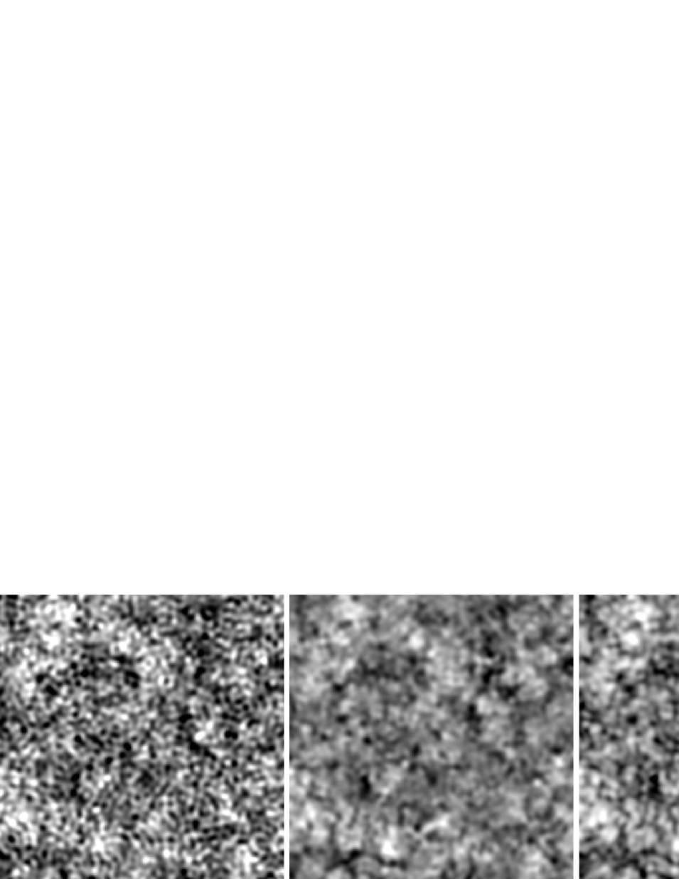
Figure 4: A simulated reconstruction of the lensing convergence using polarization and Reference Expt. C parameters. In the left panel, we display the realization of the convergence field $\kappa$ used to produce the simulated CMB. The reconstructions using the Wiener-filtered quadratic estimator and the iterative estimator are shown in the center and right panels, respectively. These frames are each $8^{\circ}32^{\prime}$ in angular width, corresponding to 1/16 of the simulated area; the scale ranges from black (diverging, $\kappa=-0.12$) through white (converging, $\kappa=+0.12$). Although all lensing multipoles up to $l=3600$ are simulated, we have only displayed the $l\leq 1600$ modes in these figures for clarity. Field rotation was neglected in the calculations for this figure.

Throughout our derivation of lensing and tensor power estimators, we have made various approximations that should be tested. The most robust way to do this is to conduct a numerical simulation of the CMB and lensing field, and then construct lensing estimators, comparing the error to the theoretical estimates of Eqs. (32) and (41). In all cases, we have used a flat sky with toroidal boundary conditions. We will only simulate the CMB polarization here; formally, the polarization-only estimators are obtained by setting ${\cal N}_{T}=\infty$ in the relevant equations.

VI.1 Reconstructing the convergence

The simplest simulations involve reconstruction of the convergence $\kappa$. We generate simulated CMB $T$, $Q$, $U$, and $\kappa$ fields on a $34^{\circ}08^{\prime}$ square patch of sky with resolution $1$ arcmin per pixel ($2048\times 2048$ pixels); lens the simulated CMB; and add appropriate noise.

We wish to compare the quadratic estimator, Eq. (40) with our new estimator, Eq. (27). The former is relatively straightforward to compute; the latter requires that we apply the methods of §III.2. We simulate Gaussian random realizations of the $Q$, $U$, and $\kappa$ fields, perform the lensing re-mapping, and add appropriate noise. We then compute the estimators of Eqs. (40) and (27). There are two tricks that are very useful in numerical computation of these estimators: first, simultaneous computation of inner products ${\bf t}^{\dagger}\sigma^{\kappa}_{\bf l}{\bf u}$ for all ${\bf l}$; and second, stochastic trace computation. We discuss each of these here.

The simultaneous computation of inner products was introduced by Refs. Hu (2001); Hu and Okamoto (2002) in order to compute quadratic estimators. A general version of this is (on a flat sky; see Ref. Okamoto and Hu (2003) for an all-sky version):

$$\sum_{\bf l}\left({l^{2}\over 2}\right)({\bf t}^{\dagger}\sigma^{\kappa}_{-{\bf l}}{\bf u})e^{i{\bf l}\cdot{\hat{\bf n}}}=\sum_{X\in\{T,Q,U\}}\nabla_{\hat{\bf n}}\cdot[t_{X}^{\ast}({\hat{\bf n}})\nabla_{\hat{\bf n}}u_{X}({\hat{\bf n}})].$$ (67)

(Note that this equation requires that ${\bf t}$ and ${\bf u}$ be written in the $\{T,Q,U\}$ basis since $E$ and $B$ have different transformation properties under lensing. Also the asterisk on $t_{X}$ is of course unnecessary if ${\bf t}$ is a real field.) If ${\bf t}$ and ${\bf u}$ are expressed in real-space, then the right-hand side is easily evaluated. The quantities ${1\over 2}l^{2}{\bf t}^{\dagger}\sigma^{\kappa}_{\bf l}{\bf u}$ are then obtained via a fast Fourier transform; division then trivially removes the $l^{2}/2$. There is a zero-wavenumber mode corresponding to $l=0$ which presents a problem for division. Here we simply set this convergence mode to zero; in the complete all-sky treatment this would be justified by noting that the convergence is $-{1\over 2}$ times the divergence of the deflection angle vector, hence $\int\kappa\,d^{2}{\hat{\bf n}}=0$ and so $\kappa_{l=0}=0$. [There is a corresponding trick for the field rotation: Eq. (67) remains valid if we make the replacements $\sigma^{\kappa}_{\bf l}\rightarrow\sigma^{\omega}_{\bf l}$ and $\nabla_{\hat{\bf n}}u_{X}({\hat{\bf n}})\rightarrow\star\nabla_{\hat{\bf n}}u_{X}({\hat{\bf n}})$.]

The trace in Eq. (27) is most easily evaluated stochastically: if we generate a random noise vector $\eta$ with covariance ${\bf N}$, then the trace is equal to the expectation value:

$${\rm Tr}\left[\Lambda_{g}^{\dagger\,-1}{\bf C}_{(0,0)}^{-1}\sigma^{\kappa}_{\bf l}{\bf C}\hat{\bf C}_{(0,0)}^{-1}\Lambda_{g}^{-1}{\bf N}\right]=\langle(\hat{\bf C}_{(0,0)}^{-1}\Lambda_{g}^{-1}\eta)^{\dagger}\sigma^{\kappa}_{\bf l}{\bf C}\hat{\bf C}_{(0,0)}^{-1}\Lambda_{g}^{-1}\eta\rangle.$$ (68)

If this Monte Carlo method is used to compute the trace, then the Monte Carlo error in its computation for one realization of $\eta$ is less than or equal to the instrument noise contribution to the uncertainty on the right-hand side of Eq. (27). [This is because the right-hand side of Eq. (27) is a quadratic function of $\hat{\bf x}$, with covariance $\hat{\bf C}$, which is greater than the noise covariance ${\bf N}$ along all directions.] Since the Monte Carlo error variance scales as the reciprocal of the number of realizations of $\eta$ used, it follows that of order a few realizations of $\eta$ are sufficient in evaluating Eq. (68). In fact for the Reference Experiments described here, we find that there is little gain in taking more than one realization of $\eta$.

Figure 5: The dependence of the mean squared error in lensing reconstruction, $\langle|\kappa_{\bf l}-\hat{\kappa}_{\bf l}|^{2}\rangle$, on the instrument parameters. The baseline is Ref. Expt. C, ${\cal N}_{P}=1.41$ $\mu$K arcmin, $\theta_{FWHM}=4$ arcmin. The thick solid line is the raw power spectrum $C^{\kappa\kappa}_{l}$; the thin solid lines indicate the mean squared error for the lensing reconstruction using the iterative estimator. As described in the text, the iterative estimator is unusable for wide-beam experiments ($\geq$10 arcmin); we used the quadratic estimator for these cases (dot-dashed curves). The dashed lines indicate the ideal zero-noise reconstruction error from the quadratic estimator according to Eq. (41) with polarization only (top) and temperature+polarization (bottom). (a) Changing ${\cal N}_{P}$; units are $\mu$K arcmin. (b) Changing $\theta_{FWHM}$; units are arcmin.

We solve Eq. (27) using the iterative procedure:

$$\kappa_{n+1,{\bf l}}^{\ast}=\zeta_{l}[\Lambda_{g}^{-1}]_{-{\bf l},-{\bf l}^{\prime}}C^{\kappa\kappa}_{l^{\prime}}\left\{(\hat{\bf C}_{(0,0)}^{-1}\Lambda_{g}^{-1}\hat{\bf x})^{\dagger}\sigma^{\kappa}_{{\bf l}^{\prime}}{\bf C}\hat{\bf C}_{(0,0)}^{-1}\Lambda_{g}^{-1}\hat{\bf x}-{\rm Tr}\left[\Lambda_{g}^{\dagger\,-1}\hat{\bf C}_{(0,0)}^{-1}\sigma^{\kappa}_{{\bf l}^{\prime}}{\bf C}\hat{\bf C}_{(0,0)}^{-1}\Lambda_{g}^{-1}{\bf N}\right]\right\}+(1-\zeta_{l})\kappa_{n,{\bf l}}^{\ast}.$$ (69)

Here $g$ is the lens configuration with convergence $\kappa$ and no rotation: $g=(\kappa,0)$, and the $\zeta_{l}$ are convergence parameters; we choose them to be:

$$\zeta_{l}=\frac{\zeta_{(c)}}{1+C^{\kappa\kappa}_{l}F^{\kappa\kappa}_{l}},$$ (70)

where $\zeta_{(c)}$ is a constant satisfying $0<\zeta_{(c)}<2$. It is found that the Wiener-filtered quadratic estimator, Eq. (40), is a good choice for initializing this iteration. The choice of $\zeta_{(c)}$ is an intricate issue: if it is set too small, the rate of convergence of the iteration becomes unacceptably slow; if it is set too high, the iteration can fail to converge entirely. The convergence can be understood by approximating Eq. (69) as linear in $\kappa_{n}$:

$$\kappa_{n+1,{\bf l}}^{\ast}\approx\zeta_{l}C_{l}^{\kappa\kappa}[{\cal F}(\kappa_{n}-\hat{\kappa})]_{\bf l}+(1-\zeta_{l})\kappa_{n,{\bf l}};$$ (71)

here we have approximated the response matrix of the likelihood gradient using the curvature matrix. Then the requirement for convergence is that all of the (possibly complex) eigenvalues of the matrix:

$$R_{{\bf l},{\bf l}^{\prime}}=\delta_{{\bf l},{\bf l}^{\prime}}-\zeta_{(c)}{C_{{\bf l},{\bf l}^{\prime}}^{\kappa\kappa\,-1}+{\cal F}_{{\bf l},{\bf l}^{\prime}}\over C_{l}^{\kappa\kappa\,-1}+F_{l}^{\kappa\kappa}}$$ (72)

lie within the unit circle. Note that, averaged over CMB+noise realizations, $\langle{\cal F}\rangle={\bf F}$, and hence $\langle{\bf R}\rangle=(1-\zeta_{(c)}){\bf 1}$; hence we conclude that the iterative procedure should be convergent for $0<\zeta_{(c)}<2$ in the absence of curvature corrections. In reality, very small values of $\zeta_{(c)}$ may be necessary for convergence, especially in cases where curvature corrections are large. Since ${\cal F}+{\bf C}^{\kappa\kappa\,-1}$ is positive definite at the maximum posterior probability point, there is always a positive value of $\zeta_{(c)}$ that results in convergence. The cases in which the small values of $\zeta_{(c)}$ are required are those in which curvature corrections are large; we have found from our simulations that these are the low-noise experiments. Convergence is generally found to be faster for the high $l$ convergence modes.

One problem we have encountered is that for experiments with low noise and wide beam ($\theta_{FWHM}\geq 10$ arcmin), the iterative estimator given by Eq. (69) is unstable. This instability arises because the noise $N_{l}$ is strongly blue; hence the de-lensing operation $\Lambda_{g}^{-1}$ in Eq. (69) mixes high-multipole noise down to lower multipoles where it disrupts the lensing estimation. This problem is in principle solvable by using the correct $({\bf C}+\Lambda_{g}^{-1}{\bf N}\Lambda_{g}^{\dagger\,-1})^{-1}$ weight function in place of ${\bf C}_{(0,0)}^{-1}$ in Eq. (23). However, since this occurs in a regime where the iterative approach does not improve upon the quadratic estimator approach anyway, we recommend simply using the quadratic estimator for wide-beam experiments.

Figure 6: The correlation coefficient $\rho=\langle\kappa\hat{\kappa}\rangle/\langle\kappa^{2}\rangle^{1/2}\langle\hat{\kappa}^{2}\rangle^{1/2}$ between the estimated and reconstructed lensing convergences as a function of multipole $l$, as determined in simulations. The correlation coefficients for the quadratic estimator are shown in panel (a); those for the iterative estimator are shown in panel (b). In both of these panels, the eight curves are for Reference Expts. A, B, C, D, E, and F (bottom to top) from Table 1. Field rotation was not included in the calculations for this figure.

We illustrate by considering the reconstruction of lensing using Reference Experiments A–F. The residual error in the reconstructed convergence $\hat{\kappa}$, as measured by computing the power spectrum of the difference $\hat{\kappa}-\kappa$ between input and reconstructed convergence maps, is shown in Fig. 3 for both quadratic and iterative estimators. For the iterative estimator applied to Ref. Expt. C, we set $\zeta_{(c)}=0.12$ in Eq. (69), used three realizations of the $\eta$ field in Eq. (68), and performed 64 iterations. Ref. Expt. F has a lower noise level and so it is necessary to use the smaller convergence parameter $\zeta_{(c)}=0.04$; the convergence is thus slower and we used 256 iterations. Ref. Expt. A has a higher noise level and so we can use $\zeta_{(c)}=0.2$ and 24 iterations. Maps of the input and reconstructed convergence fields for the Ref. Expt. C reconstruction are shown in Fig. 4. The dependence of the iterative estimator reconstruction accuracy on noise ${\cal N}_{P}$ and beam size (FWHM) $\theta_{FWHM}$ is shown in Fig. 5. We have also displayed in Fig. 5 the (theoretical) reconstruction error curves for the quadratic estimator in the absence of instrument noise. These curves represent the fundamental limit to the reconstruction accuracy possible with quadratic estimators; it is readily seen that the iterative estimator can do better if noise is low (${\cal N}_{P}<0.5$–$1$ $\mu$K arcmin, depending on the range of $l$ considered). [Note that we display $C^{\kappa\kappa}_{l}$ in these plots, whereas some authors have displayed instead $l(l+1)C^{\bf dd}/2\pi$, where ${\bf d}=\nabla\Phi$ is the deflection angle. The two are related by $l(l+1)C^{\bf dd}/2\pi=(2/\pi)C^{\kappa\kappa}_{l}$.]

The accuracy of reconstruction can also be represented by the correlation coefficient $\rho_{l}=C^{\kappa\hat{\kappa}}_{l}/\sqrt{C^{\kappa\kappa}_{l}C^{\hat{\kappa}\hat{\kappa}}_{l}}$. The correlation coefficient is the figure of merit if the objective is to cross-correlate the convergence from CMB lensing with another tracer of the density (e.g. weak lensing of galaxies), since the signal-to-noise ratio of the cross-correlation is determined by $\rho_{l}$. We have plotted the correlation coefficient in Fig. 6 for the various Reference Experiments. The iterative estimator offers improved reconstruction, especially for the lower-noise experiments (C–F).

Up until this point we have neglected the field rotation $\omega$; we should verify that this is justified. We do this by introducing field rotation with power spectrum given by Eq. (54) as computed in §IV.2 with normalization $\sigma_{8}^{\rm linear}=0.84$. We then compare the performance of the iterative estimator, Eq. (69), with and without the field rotation. The comparison is shown in Fig. 7; it is seen that the field rotation increases the mean squared error of the reconstruction by only $\sim$ 5% for Ref. Expt. E (0.5 $\mu$K arcmin noise, 2 arcmin beam) and $\sim$ 15% for Ref. Expt. F (0.25 $\mu$K arcmin noise, 2 arcmin beam).

Figure 7: The effect of field rotation on lensing estimation for Ref. Expts. E and F. (a) Power spectra of the convergence $\kappa$ (thick solid line), convergence error $\kappa-\hat{\kappa}$ with field rotation (thin solid lines), and convergence error $\kappa-\hat{\kappa}$ without field rotation (thin dashed lines). (b) The worsening of the reconstruction due to the presence of field rotation, as measured by the ratio of power spectra of the convergence errors: $\langle|(\kappa-\hat{\kappa})_{l}|^{2}\rangle_{{\rm with}\;\omega}/\langle|(\kappa-\hat{\kappa})_{l}|^{2}\rangle_{{\rm without}\;\omega}$. The same CMB, LSS, and noise (scaled appropriately to the experiment) realizations were used for all the simulations in this figure.

As a final note, we find that for low noise levels, a large number of iterations is required because our iterative process is ill-conditioned. Indeed, it is possible that there are eigenvalues of ${\bf R}$ that are so close to unity that their corresponding modes have not converged even after tens or hundreds of iterations; if this is the case, then it should be possible to improve upon our results by increasing the number of iterations, or by finding an iterative scheme that converges faster than Eq. (69). This is allowed by the Fisher matrix noise limits, which are significantly lower than the achieved noise levels (see Fig. 3). We consider this possibility unlikely since we tried increasing the number of iterations in several of the simulations and found little improvement. Additionally, modes with eigenvalue $\lambda_{\bf R}$ close to unity correspond to flat directions of the curvature matrix ${\cal F}$ [see Eq. (72)]; such directions, however, cannot be reconstructed accurately regardless of how many iterations are used.

VI.2 Extracting the convergence power spectrum

We compute the lensing power spectrum from simulated data by solving Eq. (64). The approach, once again, is iterative: we adjust the power spectrum $C^{\kappa\kappa}_{l}$ until $v_{\mu}=\langle v_{\mu}\rangle_{LSS}$. [Note that both the left and right sides of Eq. (64) depend on $C^{\kappa\kappa}_{l}$.] We will attempt here to compute the binned power spectrum, i.e. we choose a basis for the convergence power spectrum given by:

$${\cal M}_{\mu}^{l}=\left\{\begin{array}[]{lcl}1&&\mu\Delta l<l\leq(\mu+1)\Delta l,\\ 0&&{\rm otherwise},\end{array}\right.$$ (73)

where $\Delta l$ is the bin width and $\mu$ ranges from 0 through $N_{bin}-1$. We are thus attempting to reconstruct the power spectrum in $N_{bin}$ bins, equally spaced out to maximum multipole $l_{\rm max}=N_{bin}\Delta l$.

Our iterative algorithm for solving Eq. (64) is:

$$c_{\mu,n+1}=c_{\mu,n}^{1-\zeta_{(p)}}\left[c_{\mu,n}+\frac{d_{\mu}}{2\langle v_{\mu}(c_{\nu,n})\rangle_{LSS[c_{\nu,n}]}}\left(\frac{v_{\mu}(c_{\nu,n})}{\langle v_{\mu}(c_{\nu,n})\rangle_{LSS[c_{\nu,n}]}}-1\right)\right]^{\zeta_{(p)}},$$ (74)

where $n$ represents the iteration number, and $d_{\mu}$ is the number of modes that fall into the $\mu$th band. It is readily apparent that the final values $c_{\nu,\infty}$ will satisfy $v_{\mu}=\langle v_{\mu}\rangle_{LSS}$.

In order to compute the convergence power spectrum estimator, the expected value $\langle v_{\mu}(c_{\nu,n})\rangle_{LSS[c_{\nu,n}]}$ must be determined; the simplest method for doing this is via Monte Carlo simulations. Since in the end we are solving the equation $v_{\mu}=\langle v_{\mu}\rangle_{LSS}$, we want to make sure that the Monte Carlo-induced error in the right-hand side of this equation is small compared with the statistical error in the left-hand side (which depends only on the data and on $c_{\nu,n}$). It is trivial to see that after $N_{MC}$ Monte Carlo simulations, the variance in determination of the right-hand side is $1/N_{MC}$ of the statistical variance in the left-hand side. Therefore, we expect that if we use $N_{MC}$ Monte Carlo simulations to determine $\langle v_{\mu}\rangle_{LSS}$, then the variance of our determination of the convergence power spectrum will increase by a factor of $1+1/N_{MC}$. A reasonable choice, then, is to take $N_{MC}=3$, which results in 15% increase in the variance of the power spectrum estimator over the case of $N_{MC}=\infty$ (exact computation of $\langle v_{\mu}\rangle_{LSS}$). The uncertainty in the power spectrum estimation can then be estimated from Eq. (65) with the correction for $N_{MC}$:

$$\sigma_{c_{\mu}}={C^{\kappa\kappa\,2}_{l}\over C^{\kappa_{\ast}\kappa_{\ast}}_{l}}\sqrt{{2\over d_{\mu}}(1+N_{MC}^{-1})}.$$ (75)

(Note that this is the standard Gaussian formula for error bars, except that it is corrected for $N_{MC}$ and is written in terms of the filtered power spectrum $C^{\kappa_{\ast}\kappa_{\ast}}_{l}$ instead of the noise power.)

In Fig. 8(a), we show a determination of the convergence power spectrum from simulated data using Ref. Expt. C noise parameters. The choice of bins was $N_{bin}=32$, $\Delta l=50$, $l_{\rm max}=1600$, and the survey area was $0.355$ steradians ($2048$ arcmin $\times$ $2048$ arcmin, with toroidal periodic boundary conditions). We initialized the power spectrum estimation with the white spectrum $C^{\kappa\kappa}_{l}=1\times 10^{-9}$, corresponding to $c_{\mu,0}=10^{-9}$. We used $\zeta_{(p)}=0.5$ for the first two iterations of Eq. (74), which are sufficient to bring the estimated power spectrum $c_{\mu,n=2}$ to the correct order of magnitude. Once this “ballpark” estimation has been completed, we used $\zeta_{(p)}=1$ for the subsequent ($n\geq 2$) iterations.

Figure 8: (a) Simulated convergence power spectrum estimation from Ref. Expt. C with solid angle $0.355$ steradians. The solid curve is the fiducial model $C^{\kappa\kappa}_{l}$; the points are the convergence power spectrum measured from simulated data after 5 iterations. (b) The same, except that the $l\geq 1600$ convergence modes were ignored in producing the simulated data (however, exactly the same CMB+LSS+noise realization was used). The horizontal error bars indicate the widths of the bins, while the vertical error bars are the $1\sigma$ measurement uncertainties according to Eq. (75). Note that the vertical error bars include the Monte Carlo error associated with using $N_{MC}=3$ simulations to determine $\langle v_{\mu}\rangle$; if we had calculated $\langle v_{\mu}\rangle$ exactly ($N_{MC}\gg 1$), the vertical error bars would be 13% smaller (see text for details).

An examination of Fig. 8(a) shows that the power spectrum estimator Eq. (74) has been successful in reproducing the qualitative features of the power spectrum; however, the power has evidently been overestimated at the high-$l$ end. We can perform a quantitative analysis of the performance of the power spectrum estimator using the $\chi^{2}$ test, using the Gaussian error estimate of Eq. (75). The $\chi^{2}$ value for the $l<1000$ region (where the power spectrum determination should be cosmic-variance limited) is $\chi^{2}=25.46$ for $20$ degrees of freedom ($p=0.18$), indicating that Eq. (75) appears to be giving a reasonable estimate of the uncertainty on the power spectrum.

The same is not true of the high-$l$ region $1000\leq l<1600$, for which we compute $\chi^{2}=53.05$ for 12 degrees of freedom ($p=4\times 10^{-7}$). It is readily apparent from Fig. 8 that the failure of the $\chi^{2}$ test is due to an upward bias in the power spectrum estimator Eq. (74). This bias occurs because, regardless of $c_{\mu}$, our power spectrum estimator assumes that there is no convergence power at $l\geq 1600$. However, it still detects the $B$-modes induced by this short-wavelength convergence power, and introduces excess convergence power at $l<1600$ to reproduce these $B$-modes – hence $C^{\kappa\kappa}_{l}$ is overestimated. This bias can be removed by either estimating the modes to higher $l$ or including the aliasing of power from those modes into the modes we estimate as an additional source of noise Seljak (1998). This explanation of the upward bias is confirmed by Fig. 8(b), in which we have artificially “turned off” the lensing effect for convergence modes at $l\geq 1600$, then produced a simulated data set and applied the power spectrum estimator Eq. (74). In order to make the comparison between the original simulation and the restricted (i.e. short-wavelength lensing turned off) simulation as simple as possible, we have used the same CMB, noise, and LSS realizations for both. One can see by comparing Figs. 8(a) and 8(b) that there is little effect at low $l$, where the power spectrum estimation is limited by cosmic variance. However, at high $l$, one can see that the bias present in the original simulation has disappeared in the restricted simulation, thereby confirming that the bias was due to high-$l$ convergence power. The $\chi^{2}$ for the $1000\leq l<1600$ range has been reduced to $\chi^{2}=31.36$ (12 degrees of freedom, $p=1.7\times 10^{-3}$), which is still indicative of underestimation of the uncertainty in the $c_{\mu}$. Thus we conclude that in this regime, either the Gaussian error estimate Eq. (75) is underestimating the error by a factor of $\sim\sqrt{31/12}\approx 1.6$, or the error bars are correlated, or the iteration of Eq. (74) has not completely converged.

In a real lensing experiment, the underlying primary power spectrum $C^{EE}_{l}$ is unknown and only the lensed power spectrum is directly observable (and even our knowledge of this is limited by instrument noise and cosmic variance). Thus a slightly more complicated version of the above analysis will be necessary to simultaneously solve for $C^{EE}_{l}$ and $C^{\kappa\kappa}_{l}$. (Although since in the regime we are examining, $l<3000$, the $E$ power spectrum is dominated by primary anisotropies rather than lensing, we do not expect a degeneracy between these two quantities.) It will also be necessary to estimate the convergence power spectrum well beyond the region of interest in order to avoid the upward bias described here. Since the signal-to-noise ratio at high $l$ is low, it will be necessary to use wider bins (i.e. larger $\Delta l$) in this region. The choice of exactly which bins to use must be determined by the characteristics of the specific experiment.

VII Conclusions

Weak gravitational lensing of the CMB allows us to reconstruct the (projected) mass distribution in the universe, thereby probing large-scale structure and its power spectrum. Since the window functions for lensing peak at redshift $z$ of order unity, lensing offers the possibility of using the CMB to study the low-redshift universe Zaldarriaga and Seljak (1999); Seljak and Zaldarriaga (1999a); Hu (2001); Benabed et al. (2001); Bernardeau (1997). “Cleaning” of lensing from CMB maps is potentially valuable for studying the primary CMB, particularly for inflationary gravitational wave searches using the low-$l$ $B$-mode polarization Knox and Song (2002); Kesden et al. (2002). Since the primary CMB polarization is expected to contain only $E$-modes on the relevant angular scales ($l$ of order $10^{3}$), while lensing transfers some of the CMB polarization power into $B$-modes Zaldarriaga and Seljak (1998), all $B$-modes that we see on these scales are due to lensing (or foregrounds). Thus the CMB $B$-mode polarization allows much better lensing reconstruction than is possible using temperature data alone. It is thus of interest to consider optimal methods of reconstructing the lensing field from CMB polarization data; in this paper, we have investigated this problem in detail and improved significantly on the previous quadratic estimator methods Hu and Okamoto (2002). We have shown that this improvement can be up to an order of magnitude in mean squared error over the zero-noise reconstruction error for the quadratic estimator.

We make several comments concerning the present calculations. First of all, our lensing estimator, Eq. (21), while statistically superior to the quadratic estimator, still does not achieve the Cramer-Rao bound on reconstruction accuracy. We have argued that this results in part from “curvature corrections,” fluctuations in the curvature matrix that render the Cramer-Rao bound impossible to achieve (more generally, this should also serve as a warning against blindly assuming that the statistical errors in any measurement are given by ${\bf F}^{-1}$.). We expect that our lensing reconstruction estimator is near-optimal since it is an approximation to the maximum-likelihood estimator and our iterative estimator shows no signs of incomplete convergence, however the possibility of further improvement has not been ruled out.

Secondly, we have assumed negligible primary $B$ mode polarization here (although the formalism described herein is trivially modified to include significant primary $B$-modes, the results would be qualitatively different). In the absence of vector or tensor perturbations, this is correct; if vector or tensor perturbations are present, then one must consider their effect on lensing reconstruction. In the case of inflationary gravitational waves, primary $B$-modes are generated mostly on very large angular scales; the arcminute-scale anisotropies used for lensing reconstruction are uncontaminated Hu and Okamoto (2002). (Formally, if we were doing a lensing reconstruction with the objective of cleaning lensing contamination of the tensor-induced reionization bump at $l<20$, we would set $N^{BB}_{l}=\infty$ for $l<20$ so that the lensing reconstruction does not remove tensor $B$-modes.) A more rigorous investigation of the effect on inflationary gravitational wave searches is deferred to future work.

Thirdly, the real CMB is contaminated by foregrounds – an important issue for all CMB anisotropy experiments. One advantage of using CMB polarization for lensing reconstruction is that whereas the small-scale CMB temperature field is heavily contaminated by scattering-induced secondary anisotropies such as the thermal and kinetic Sunyaev-Zel’dovich effects, Ostriker-Vishniac effect, and patchy reionization, these effects are much smaller for polarization Hu (2000b). However, polarized point sources and galactic foregrounds are still a serious concern. These have very different frequency dependence than the blackbody fluctuations characteristic of the CMB, and this property has been exploited to remove them; unfortunately, their fluctuation spectrum, degree of polarization, non-Gaussianity, and variations in frequency dependence are poorly understood. Galactic foregrounds do not correlate with the cosmological signals, and in this sense the residuals from their subtraction act like instrument noise contaminating the $B$-mode (and, to a lesser extent, $E$-mode) polarization. The foreground power spectrum is likely to be different from that of instrument noise and is variable across the sky; nevertheless, if the covariance matrix of the foregrounds (or residuals after foreground subtraction) can be determined, then we can add the foreground covariance to the instrument noise covariance matrix ${\bf N}$. (If the statistical properties of the foreground residuals cannot be determined or at least constrained, then any cosmological analysis is pointless regardless of the methods used.) Polarized point sources produce Poisson noise; also since many of them are extragalactic, one could be concerned about their correlation with LSS and hence the lensing signal. We leave a detailed study of foregrounds and their impact on lensing reconstruction to future investigation. We note that the predicted levels of foreground contamination from dust and synchrotron galactic emission are at a level of a few $\mu$K arcmin prior to any frequency cleaning Tegmark et al. (2000), comparable to the noise levels discussed here. Frequency cleaning should reduce this, at the expense of amplifying instrument noise. If foreground removal is inadequate, this may result in anomalies in the final results such as unphysical correlations between the convergence maps and CMB polarization, variation of the convergence power spectrum between “clean” and “dirty” portions of the sky, correlation of the convergence maps with synchrotron or dust emission, etc.

In summary, we have shown that taking into account the full likelihood function allows improved reconstruction of the lensing of the CMB polarization field over that achieved by quadratic statistics. For purposes of computing the lensing power spectrum or cross-correlating CMB lensing with another tracer of the cosmological density field, the most important improvement is at high $l$ where earlier approaches do not reconstruct the convergence at high signal-to-noise. (At low $l$, the reconstruction is already cosmic variance limited.) If one’s objective is to clean out the lensing effect in search of primordial gravitational waves, then the relevant quantity is the residual error in the reconstruction, and it is important to reduce this even if the convergence has been mapped at high signal-to-noise; hence improvement at all multipoles is useful. We conclude that the likelihood-based estimators developed here offer the best prospective so far to extract the full amount of information from future high-resolution CMB polarization experiments.

Appendix A Quadratic estimator

In our simulations, we have compared the error of our iterative estimator, Eq. (27), with that of the quadratic estimator, Eq. (40). Here we show that the latter estimator corresponds to the optimally weighted quadratic estimator, as proposed by Ref. Hu and Okamoto (2002). Statistically isotropic noise is assumed throughout.

We begin by expanding Eq. (41) using the formula for ${\bf f}^{\kappa}_{\bf l}$ given by Eq. (36). The off-diagonal elements vanish by symmetry, while the diagonal elements are:

$$F_{l}^{\rm(quad)}={1\over 2}\sum_{{\bf l}_{1}}{\rm Tr}\left\{[{\bf f}^{\kappa}_{-{\bf l}}]_{-{\bf l}_{1},{\bf l}_{2}}[\langle\hat{\bf C}\rangle_{LSS}]_{l_{2}}^{-1}[{\bf f}^{\kappa}_{\bf l}]_{{\bf l}_{2},-{\bf l}_{1}}[\langle\hat{\bf C}\rangle_{LSS}]_{l_{1}}^{-1}\right\},$$ (76)

where we have defined ${\bf l}_{2}={\bf l}-{\bf l}_{1}$, and the inverses are $3\times 3$ matrix inverses (using the $\{T,E,B\}$ basis). Next we note that to first order in $\kappa$, the correlation between two Fourier modes of temperature or polarization is:

$$\langle\hat{\bf x}_{{\bf l}_{1}}\hat{\bf x}_{-{\bf l}_{2}}^{\dagger}\rangle=[{\bf f}^{\kappa}_{\bf l}]_{{\bf l}_{1},-{\bf l}_{2}}\kappa_{\bf l}+O(\kappa^{2}).$$ (77)

A general quadratic estimator for the convergence $\kappa$ is then constructed as:

$$\hat{\kappa}_{\bf l}=\sum_{{\bf l}_{1}}\hat{\bf x}_{-{\bf l}_{2}}^{\dagger}[\Xi_{-{\bf l}}]_{-{\bf l}_{2},{\bf l}_{1}}\hat{\bf x}_{{\bf l}_{1}},$$ (78)

where $\Xi_{-{\bf l}}$ is the weight matrix, which we assume without loss of generality to be Hermitian (since the anti-Hermitian part does not contribute to $\hat{\kappa}_{\bf l}$). We further require it to satisfy $[\Xi_{-{\bf l}}]_{-{\bf l}_{2},{\bf l}_{1}}=[\Xi_{\bf l}]_{{\bf l}_{2},-{\bf l}_{1}}^{\dagger}$. (This guarantees that the estimate $\hat{\kappa}$ is a real field.) We can construct the optimally weighted unbiased (to first order) estimator for $\kappa$ by minimizing the variance of the estimator (neglecting the trispectrum contribution):

$$V_{l}=\langle|\hat{\kappa}_{\bf l}|^{2}\rangle_{LSS}\approx\sum_{{\bf l}_{1}}{\rm Tr}\left\{[\langle\hat{\bf C}\rangle_{LSS}]_{l_{2}}[\Xi_{-{\bf l}}]_{-{\bf l}_{2},{\bf l}_{1}}[\langle\hat{\bf C}\rangle_{LSS}]_{l_{1}}[\Xi_{\bf l}]_{{\bf l}_{1},-{\bf l}_{2}}\right\},$$ (79)

subject to the constraint that the estimator be unbiased to first-order (i.e. have unit response):

$$1=\sum_{{\bf l}_{1}}{\rm Tr}\left\{[{\bf f}^{\kappa}_{\bf l}]_{{\bf l}_{1},-{\bf l}_{2}}[\Xi_{-{\bf l}}]_{-{\bf l}_{2},{\bf l}_{1}}\right\}.$$ (80)

We may compute the minimum of Eq. (79) constrained by Eq. (80) using the method of Lagrange multipliers. The equation $\delta V_{l}+\lambda^{-1}\delta 1=0$ becomes:

$$\sum_{{\bf l}_{1}}{\rm Tr}\left\{2[\langle\hat{\bf C}\rangle_{LSS}]_{l_{2}}[\delta\Xi_{-{\bf l}}]_{-{\bf l}_{2},{\bf l}_{1}}[\langle\hat{\bf C}\rangle_{LSS}]_{l_{1}}[\Xi_{\bf l}]_{{\bf l}_{1},-{\bf l}_{2}}+\frac{1}{\lambda}[{\bf f}^{\kappa}_{\bf l}]_{{\bf l}_{1},-{\bf l}_{2}}[\delta\Xi_{-{\bf l}}]_{-{\bf l}_{2},{\bf l}_{1}}\right\}=0.$$ (81)

The solution to this (allowing $\delta\Xi_{-{\bf l}}$ to be arbitrary) is:

$$[\Xi_{-{\bf l}}]_{-{\bf l}_{2},{\bf l}_{1}}={1\over 2\lambda}[\langle\hat{\bf C}\rangle_{LSS}]_{l_{2}}^{-1}[{\bf f}^{\kappa}_{\bf l}]_{{\bf l}_{2},-{\bf l}_{1}}[\langle\hat{\bf C}\rangle_{LSS}]_{l_{1}}^{-1}.$$ (82)

The correct normalization $\lambda$ is obtained by substitution into Eq. (80); it is easily seen to be $\lambda=F_{l}^{\rm(quad)}$. The variance of this estimator in the absence of lensing, determined by substitution into Eq. (79), is $1/F_{l}^{\rm(quad)}$. The quadratic estimator we have used, Eq. (40), is then seen to be a Wiener-filtered version of Eq. (82) with the optimized choice for $\Xi$, Eq. (82), and its covariance Eq. (42) then follows from the theory of Wiener-filtering.

Hu and Okamoto Hu and Okamoto (2002) derive a quadratic estimator using essentially the same method outlined in this appendix. While they have chosen to separately optimize the different components of $\Xi$ ($TT$, $TE$, $EE$, $TB$, and $EB$) and then combine these to form a “minimum variance” estimator, the end result of the optimal filtering must be the same. (Note that while our covariance response function ${\bf f}$ is the same as Hu and Okamoto’s ${\bf f}$ aside from a factor of $l^{2}/2$ due to use of $\Phi$ vs. $\kappa$ as the fundamental field, we have used $\Xi$ in place of their $F/A$ to avoid confusion with the Fisher matrix.)

Appendix B Lensing $B$-modes and idealized reconstruction

The purpose of this Appendix is to investigate the question of whether, in the absence of noise and field rotation, the equation $B_{\rm unlensed}=0$ could be used to completely reconstruct the convergence field. We show that with probability 1, it is possible to reconstruct most of the convergence modes. There may remain a small number of convergence modes that cannot be reconstructed by this method. If we impose periodic boundary conditions, the fraction of the convergence modes that are in this category is at most of order $1/l_{\rm max}$; however, there may be fewer of these degenerate modes, or possibly none at all. We have not investigated more realistic survey topologies but we would expect the general result to be similar on scales small compared to the angular width of the survey. However, this seems mostly an academic point since zero noise is of course unrealistic, and there can be many almost-degenerate modes that spoil a reconstruction based on $B_{\rm unlensed}=0$.

The $B$-mode induced by lensing is, to first order:

$$B_{{\bf l},\rm lensing}={1\over\sqrt{4\pi}}\sum_{{\bf l}^{\prime}}\left(\frac{2}{l^{\prime}{{}^{2}}}\right){\bf l}^{\prime}\cdot({\bf l}-{\bf l}^{\prime})\sin 2\alpha\;E_{{\bf l}-{\bf l}^{\prime}}\kappa_{{\bf l}^{\prime}}=\sum_{{\bf l}^{\prime}}{\cal T}_{{\bf l},{\bf l}^{\prime}}\kappa_{{\bf l}^{\prime}},$$ (83)

where ${\cal T}$ is a transfer matrix that is a linear function of $E$ (and once again $\alpha=\phi_{\bf l}-\phi_{{\bf l}^{\prime}}$). In the absence of noise, we may set $B_{{\bf l},\rm lensing}$ equal to the observed polarization $\hat{B}_{\bf l}$. We see that if $N$ Fourier modes are considered, there are $N$ linear equations for $N$ unknowns $\kappa_{\bf l}$. (We do not consider ${\bf l}=0$ modes since there does not exist a $\kappa_{0}$ mode, and lensing has no effect on zero-wavenumber CMB modes.) Thus any convergence mode that cannot be reconstructed must be associated with a degenerate direction of ${\cal T}$. It is clear that for some realizations of the primary CMB, e.g. $E=0$, ${\cal T}$ is massively degenerate. We thus wish to explore whether these singular realizations are “likely” or have probability zero. We will assume here that $C^{EE}_{l}>0$ for all of the $E$-modes so that “probability zero” and “measure zero” can be taken to be equivalent.

In order to do this, we consider the characteristic polynomial of ${\cal T}$:

$$P(\lambda;E)=\det({\cal T}-\lambda{\bf 1})=\sum_{n=0}^{N}a_{n}(E)\lambda^{n}.$$ (84)

The determinant of an $N\times N$ matrix is a polynomial of degree $N$ in the entries of the matrix, hence each $a_{n}(E)$ is a polynomial of order at most $N-n$ in the $E_{\bf l}$. We know from linear algebra that the roots and multiplicities of $P(\lambda;E)$ (viewed as a polynomial in $\lambda$) are precisely the eigenvalues and multiplicities of ${\cal T}$; in particular, the number of degenerate ($\lambda=0$) modes is equal to the smallest value of $n$ for which $a_{n}(E)\neq 0$. Now suppose it were the case for some $n$ that $a_{n}(E)\neq 0$ with nonzero probability (recall that the primary CMB polarization $E$ is a random variable). This implies that $a_{n}(E)\neq 0$ is generic, i.e. only a small (measure zero) set of values of $E$ give $a_{n}(E)=0$. The significance of this result is that if we can exhibit even one possible polarization field $E$ for which $a_{n}(E)\neq 0$, it follows that $a_{n}(E)\neq 0$ with unit probability for the real primary CMB polarization field. A similar statement holds for the number of degenerate convergence modes: if we can exhibit a possible polarization field with $n$ degenerate modes, then it follows that with unit probability, the lensing field as reconstructed from the real CMB will have at most $n$ degenerate modes. Conceptually, this means that the generic lensing reconstruction using $B_{\rm unlensed}=0$ cannot be more degenerate than any special case we exhibit. (It may, however, be less degenerate.)

We consider here the following very simple realization: take a sky with area $4\pi$, square (with side length $\sqrt{4\pi}$), and with periodic boundary conditions. Suppose that only the $E$-mode $E_{\bf L}$ where ${\bf L}=(2\pi/\sqrt{4\pi},0)$ (i.e. the longest-wavelength mode in the $x$-direction) is nonzero. Now consider a degenerate convergence mode, i.e. one that does not contribute to $B_{\rm lensing}$. From Eq. (83), we see that the $B=0$ requirement forces all of the convergence modes $\kappa_{{\bf l}^{\prime}}$ to be zero except those for which $\sin 2\alpha=0$, i.e. those for which ${\bf l}^{\prime}$ is either parallel to or perpendicular to ${\bf l}^{\prime}+{\bf L}$. The latter is impossible given the boundary conditions and the former requires ${\bf l}^{\prime}$ to lie in the $x$-direction. Thus, out of $O(l_{\rm max}^{2})$ convergence modes, only the $O(l_{\rm max})$ modes with wavevector in the $x$-direction cannot be reconstructed. Hence no more than a fraction $O(1/l_{\rm max})$ of the convergence modes are degenerate (i.e. cannot be reconstructed from $B_{\rm unlensed}=0$), and by the argument of the previous paragraph this must hold with probability 1 for the actual realization of the primary polarization field. Note that this is only an upper limit and the actual number of degenerate modes may be smaller, or even zero.

The problem of lensing reconstruction using $B_{\rm unlensed}=0$ has been considered previously using real-space methods by Ref. Benabed et al. (2001). They derive the following equation for the lensing-induced $B$-mode:

$${1\over 2}\nabla^{2}B_{\rm lensing}=\gamma_{U}\nabla^{2}Q-\gamma_{Q}\nabla^{2}U+\nabla\gamma_{U}\cdot\nabla Q-\nabla\gamma_{Q}\cdot\nabla U,$$ (85)

where (as above) $\gamma_{Q}$ and $\gamma_{U}$ are second derivatives of $\Phi$. This is therefore a third-order partial differential equation for $\Phi$. Ref. Benabed et al. (2001) then performs a two-dimensional Taylor-expansion of $\Phi$ and finds that some of the coefficients are not fixed by Eq. (85). They thus determine that there exists a class of lensing potential modes that do not produce $B$-modes purely by counting the number of equations and the number of variables to be calculated. The relationship between our approach and that of Ref. Benabed et al. (2001) is that we express ${\cal T}$ in the Fourier basis (Eq. 83), whereas they have expressed ${\cal T}$ in the Taylor polynomial $\{x^{j}y^{k}\}_{j,k=0}^{\infty}$ basis. These bases are not equivalent due to the differing boundary conditions assumed (the Fourier basis imposes periodic boundary conditions whereas the Taylor polynomial basis does not), and this leads to different conclusions regarding the number and character of degenerate modes. In the Fourier basis there are the same number of equations as variables. Thus one cannot conclude from the counting argument alone that there is a degeneracy in the case of full-sky coverage. (The analysis on the sphere would be slightly more intricate since the sky is curved and the boundary conditions have different topology than in the flat-sky approximation; however, on scales $l\gg 1$ small compared to the curvature scale, we expect that the results presented here will still apply.)

Appendix C Curvature corrections

Our purpose in this Appendix is to investigate in greater detail the mathematical structure of the curvature corrections, i.e. the increase in uncertainty in lensing reconstruction due to fluctuations of the curvature matrix. We show that the curvature correction has another interpretation: it represents the increased noise in the reconstruction of $\kappa_{\bf l}$ due to the presence of other lensing modes, $\kappa_{{\bf l}^{\prime}}$ (where ${\bf l}^{\prime}\neq\pm{\bf l}$), an effect studied in detail in Kesden et al Kesden et al. (2003), where it was called the “first-order noise contribution” and denoted by $N^{(1)}_{XX^{\prime},X^{\prime\prime}X^{\prime\prime\prime}}(L)$. Here we show that in fact the curvature correction contains the likelihood analysis manifestation of the $N^{(1)}$ of Ref. Kesden et al. (2003).

We can compute the curvature corrections to this as follows. If we define $\delta{\cal F}={\cal F}-{\bf F}$, and retain our approximation from Eq. (32) that ${\bf F}$ is independent of $\kappa$, then we have:

$${\bf S}=\langle(\delta{\cal F}+{\bf F}+{\bf C}^{\kappa\kappa\,-1})^{-1}\rangle_{LSS}\sim{\bf S}_{0}+{\bf S}_{0}\langle\delta{\cal F}\;{\bf S}_{0}\;\delta{\cal F}\rangle_{LSS}{\bf S}_{0}-...,$$ (86)

where ${\bf S}_{0}=({\bf F}+{\bf C}^{\kappa\kappa\,-1})^{-1}$. [To derive this equation, we have merely Taylor-expanded in $\delta{\cal F}$, then taken the CMB+noise+LSS ensemble average, and noted that by definition $\delta{\cal F}$ vanishes when ensemble-averaged over CMB+noise realizations. Note that because we have taken the expectation value, Eq. (86) should be viewed as an asymptotic expansion rather than a Taylor expansion.] The mean squared error ${\bf S}$ picks up “curvature correction” terms involving $\delta{\cal F}$ that cause it to not equal the naive result ${\bf S}_{0}$. Note that curvature corrections to ${\bf S}$ only increase ${\bf S}$, they cannot decrease it (in the sense that ${\bf S}-{\bf S}_{0}$ has all eigenvalues $\geq 0$; equivalently the diagonal elements ${\bf S}_{jj}\geq[{\bf S}_{0}]_{jj}$ in all orthonormal bases). This is true to all orders in $\delta{\cal F}$ because the inverse of the mean of a set of positive definite Hermitian matrices is smaller than the mean of the inverses (in this same sense).

In order to compute the second-order curvature correction explicitly, we must understand the fluctuations in the curvature matrix. For simplicity, we evaluate $\delta{\cal F}$ at $\kappa=0$. In this case, we find:

$${\cal F}_{{\bf l},{\bf l}^{\prime}}\equiv {\cal F}[\kappa_{\bf l},\kappa_{{\bf l}^{\prime}}]={\partial^{2}\over\partial\kappa_{\bf l}^{\ast}\partial\kappa_{{\bf l}^{\prime}}}\left({1\over 2}\ln\det\hat{\bf C}_{g}+{1\over 2}\hat{\bf x}^{\dagger}\hat{\bf C}_{g}^{-1}{\bf x}\right)$$

$$= {1\over 2}\hat{\bf x}^{\dagger}\hat{\bf C}^{-1}\left(2{\partial\hat{\bf C}\over\partial\kappa_{-{\bf l}}}\hat{\bf C}^{-1}{\partial\hat{\bf C}\over\partial\kappa_{{\bf l}^{\prime}}}-{\partial^{2}\hat{\bf C}\over\partial\kappa_{-{\bf l}}\partial\kappa_{{\bf l}^{\prime}}}\right)\hat{\bf C}^{-1}\hat{\bf x}-{1\over 2}{\rm Tr}\left[\hat{\bf C}^{-1}\left({\partial\hat{\bf C}\over\partial\kappa_{-{\bf l}}}\hat{\bf C}^{-1}{\partial\hat{\bf C}\over\partial\kappa_{{\bf l}^{\prime}}}-{\partial^{2}\hat{\bf C}\over\partial\kappa_{-{\bf l}}\partial\kappa_{{\bf l}^{\prime}}}\right)\right],$$ (87)

where the second line has the $\hat{\bf C}$’s evaluated at $\kappa=0$. Subtracting out the average value ${\bf F}_{{\bf l},{\bf l}^{\prime}}$ over CMB+noise realizations yields:

$$\delta{\cal F}_{{\bf l},{\bf l}^{\prime}}=-{1\over 2}\hat{\bf x}^{\dagger}\hat{\bf C}^{-1}{\bf J}_{(-{\bf l},{\bf l}^{\prime})}\hat{\bf C}^{-1}\hat{\bf x}+{1\over 2}{\rm Tr}\left(\hat{\bf C}^{-1}{\bf J}_{(-{\bf l},{\bf l}^{\prime})}\right),$$ (88)

where we have defined:

$${\bf J}_{(-{\bf l},{\bf l}^{\prime})}=\left.\hat{\bf C}{\partial^{2}[\hat{\bf C}^{-1}]\over\partial\kappa_{-{\bf l}}\partial\kappa_{{\bf l}^{\prime}}}\hat{\bf C}\right|_{\kappa=0}=\left.\left({\partial\hat{\bf C}\over\partial\kappa_{-{\bf l}}}\hat{\bf C}^{-1}{\partial\hat{\bf C}\over\partial\kappa_{{\bf l}^{\prime}}}+{\partial\hat{\bf C}\over\partial\kappa_{{\bf l}^{\prime}}}\hat{\bf C}^{-1}{\partial\hat{\bf C}\over\partial\kappa_{-{\bf l}}}-{\partial^{2}\hat{\bf C}\over\partial\kappa_{-{\bf l}}\partial\kappa_{{\bf l}^{\prime}}}\right)\right|_{\kappa=0}.$$ (89)

Note that ${\bf J}_{(-{\bf l},{\bf l}^{\prime})}={\bf J}_{({\bf l}^{\prime},-{\bf l})}={\bf J}_{({\bf l},-{\bf l}^{\prime})}^{\dagger}$.

Using this relation, and noting that at $\kappa=0$ we have $\partial\hat{\bf C}/\partial\kappa_{\bf l}={\bf f}^{\kappa}_{\bf l}$, we can use Wick’s theorem to compute:

$$\langle\delta{\cal F}_{{\bf l},{\bf l}^{\prime}}\delta{\cal F}_{{\bf l}_{1},{\bf l}^{\prime}_{1}}\rangle={1\over 4}{\rm Tr}\left(\hat{\bf C}^{-1}{\bf J}_{(-{\bf l},{\bf l}^{\prime})}\hat{\bf C}^{-1}{\bf J}_{(-{\bf l}^{\prime},{\bf l})}\right).$$ (90)

In the case of statistically isotropic noise, Eq. (90) allows us to compute the covariance of the reconstruction ${\bf S}$ using Eq. (86). In harmonic space, the off-diagonal elements of ${\bf S}$ vanish by symmetry whereas the diagonal elements are given by:

$$S_{l}=[S_{0}]_{l}+{1\over 4}[S_{0}]_{l}^{2}\sum_{{\bf l}^{\prime}}[S_{0}]_{l^{\prime}}{\rm Tr}\left(\hat{\bf C}^{-1}{\bf J}_{(-{\bf l},{\bf l}^{\prime})}\hat{\bf C}^{-1}{\bf J}_{(-{\bf l}^{\prime},{\bf l})}\right),$$ (91)

which is a summation over quadrilateral configurations of the modes ${\bf l}$, ${\bf l}^{\prime}$, and the mode over which we sum when computing the trace.

To lowest order ($\delta{\cal F}^{2}$), the curvature correction is given by Eq. (91). The correction to the mean inverse curvature $V_{l}$, i.e. to the covariance matrix of an unbiased estimator for $\kappa$, is related to the correction to $S_{l}$ by noting that $S_{l}^{-1}=V_{l}^{-1}+C_{l}^{\kappa\kappa\,-1}$, hence:

$$\Delta V_{l}=\frac{V_{l}^{2}}{S_{l}^{2}}\Delta S_{l}\approx{1\over 4}V_{l}^{2}\sum_{{\bf l}^{\prime}}[S_{0}]_{l^{\prime}}{\rm Tr}\left(\hat{\bf C}^{-1}{\bf J}_{(-{\bf l},{\bf l}^{\prime})}\hat{\bf C}^{-1}{\bf J}_{(-{\bf l}^{\prime},{\bf l})}\right).$$ (92)

We now pass to the “linear approximation” in which the second derivative $\partial^{2}\hat{\bf C}/\partial\kappa_{\bf l}^{\ast}\partial\kappa_{{\bf l}^{\prime}}$ is neglected. (This was found to be a valid approximation for temperature-based lensing estimation on scales $l<3500$ Hirata and Seljak (2003), although it is unclear whether this is also true in the present context.) Substituting Eq. (89) then yields:

$$\Delta V_{l}\approx{1\over 2}V_{l}^{2}\sum_{{\bf l}^{\prime}}[S_{0}]_{l^{\prime}}{\rm Tr}\left(\hat{\bf C}^{-1}{\bf f}_{{\bf l}}^{\kappa}\hat{\bf C}^{-1}{\bf f}_{{\bf l}^{\prime}}^{\kappa}\hat{\bf C}^{-1}{\bf f}_{-{\bf l}}^{\kappa}\hat{\bf C}^{-1}{\bf f}_{-{\bf l}^{\prime}}^{\kappa}+\hat{\bf C}^{-1}{\bf f}_{{\bf l}}^{\kappa}\hat{\bf C}^{-1}{\bf f}_{-{\bf l}}^{\kappa}\hat{\bf C}^{-1}{\bf f}_{{\bf l}^{\prime}}^{\kappa}\hat{\bf C}^{-1}{\bf f}_{-{\bf l}^{\prime}}^{\kappa}\right).$$ (93)

This should be compared with the first-order noise contribution $N^{(1)}$ of Ref. Kesden et al. (2003). In our notation, and written in terms of the convergence rather than the potential, their Eq. (25) can be re-written with the help of some algebra and the relation ${\bf f}^{\kappa}_{\bf l}={\bf f}_{-{\bf l}}^{\kappa\,\dagger}$ as:

$$N^{(1)}_{TT,TT}(\kappa_{\bf l})={1\over 2}V_{l}^{2}\sum_{{\bf l}^{\prime}}C^{\kappa\kappa}_{l^{\prime}}\sum_{{\bf l}_{1}}\frac{[f_{\bf l}]_{{\bf l}_{1},-{\bf l}_{2}}^{\kappa}[f_{{\bf l}^{\prime}}]_{-{\bf l}_{2},-{\bf l}_{2}-{\bf l}^{\prime}}^{\kappa}[f_{-{\bf l}}]_{-{\bf l}_{2}-{\bf l}^{\prime},{\bf l}_{1}-{\bf l}^{\prime}}^{\kappa}[f_{-{\bf l}^{\prime}}]_{{\bf l}_{1}-{\bf l}^{\prime},{\bf l}_{1}}^{\kappa}}{[\langle\hat{\bf C}\rangle_{LSS}]_{l_{1}}^{\kappa}[\langle\hat{\bf C}\rangle_{LSS}]_{l_{2}}^{\kappa}[\langle\hat{\bf C}\rangle_{LSS}]_{{\bf l}_{2}+{\bf l}^{\prime}}^{\kappa}[\langle\hat{\bf C}\rangle_{LSS}]_{{\bf l}_{1}-{\bf l}^{\prime}}^{\kappa}}.$$ (94)

This is the first term of Eq. (93), except that it only includes temperature information (hence we have multiplication of numbers rather than $3\times 3$ matrices), and the residual power spectrum $[S_{0}]_{l^{\prime}}$ has been replaced with the raw convergence power spectrum $C^{\kappa\kappa}_{l^{\prime}}$. (The latter difference arises because Ref. Kesden et al. (2003) computed the first-order noise $N^{(1)}$ for the quadratic estimator; when the Bayesian estimator is used, the contaminating modes $\{\kappa_{{\bf l}^{\prime}}\}$ have their power reduced from $C^{\kappa\kappa}_{l^{\prime}}$ to $[S_{0}]_{l^{\prime}}$ since the estimated lensing field $\hat{\kappa}$ is used to de-lens the CMB.) Thus we see that the first-order noise arises in the likelihood formalism as a curvature correction, which is not taken into account in the Fisher matrix for lensing reconstruction.

The question naturally arises as to the interpretation of the second term in the curvature correction, Eq. (93). We note that within the linear approximation,

$$\langle\hat{\bf C}^{-1}\rangle_{LSS}=\hat{\bf C}_{(0,0)}^{-1}+\sum_{{\bf l}^{\prime}}[S_{0}]_{{\bf l}^{\prime}}\hat{\bf C}_{(0,0)}^{-1}{\bf f}^{\kappa}_{{\bf l}^{\prime}}\hat{\bf C}_{(0,0)}^{-1}{\bf f}_{-{\bf l}^{\prime}}^{\kappa}\hat{\bf C}_{(0,0)}^{-1}.$$ (95)

The second term of Eq. (93) is thus seen to be the correction to the Fisher matrix, Eq. (32), due to the lensing effect on the CMB power spectrum.

References

- Bernardeau (1997) F. Bernardeau, A&A 324, 15 (1997).
- Zaldarriaga and Seljak (1999) M. Zaldarriaga and U. Seljak, Phys. Rev. D 59, 123507 (1999).
- Seljak and Zaldarriaga (1999a) U. Seljak and M. Zaldarriaga, Phys. Rev. Lett. 82, 2636 (1999a).
- Hu (2001) W. Hu, Astrophys. J. 557, L79 (2001).
- Benabed et al. (2001) K. Benabed, F. Bernardeau, and L. van Waerbeke, Phys. Rev. D 63, 43501 (2001).
- Peiris and Spergel (2000) H. V. Peiris and D. N. Spergel, Astrophys. J. 540, 605 (2000).
- Goldberg and Spergel (1999) D. M. Goldberg and D. N. Spergel, Phys. Rev. D 59, 103002 (1999).
- Seljak and Zaldarriaga (1999b) U. Seljak and M. Zaldarriaga, Phys. Rev. D 60, 43504 (1999b).
- Zaldarriaga and Seljak (1998) M. Zaldarriaga and U. Seljak, Phys. Rev. D 58, 23003 (1998).
- Hu and Okamoto (2002) W. Hu and T. Okamoto, Astrophys. J. 574, 566 (2002).
- Knox and Song (2002) L. Knox and Y. Song, Phys. Rev. Lett. 89, 11303 (2002).
- Kesden et al. (2002) M. Kesden, A. Cooray, and M. Kamionkowski, Phys. Rev. Lett. 89, 11304 (2002).
- Cole and Efstathiou (1989) S. Cole and G. Efstathiou, MNRAS 239, 195 (1989).
- Seljak (1996) U. Seljak, Astrophys. J. 463, 1 (1996).
- Guzik et al. (2000) J. Guzik, U. Seljak, and M. Zaldarriaga, Phys. Rev. D 62, 043517 (2000).
- Zaldarriaga (2000) M. Zaldarriaga, Phys. Rev. D 62, 63510 (2000).
- Hirata and Seljak (2003) C. M. Hirata and U. Seljak, Phys. Rev. D 67, 43001 (2003).
- Seljak and Zaldarriaga (2000) U. Seljak and M. Zaldarriaga, Astrophys. J. 538, 57 (2000).
- Hu (2000a) W. Hu, Phys. Rev. D 62, 43007 (2000a).
- Seljak and Zaldarriaga (1996) U. Seljak and M. Zaldarriaga, Astrophys. J. 469, 437 (1996).
- Kesden et al. (2003) M. Kesden, A. Cooray, and M. Kamionkowski, ArXiv Astrophysics e-prints astro-ph/0302536 (2003).
- Cooray and Hu (2002) A. Cooray and W. Hu, Astrophys. J. 574, 19 (2002).
- Carroll et al. (1992) S. M. Carroll, W. H. Press, and E. L. Turner, ARA&A 30, 499 (1992).
- Peacock and Dodds (1996) J. A. Peacock and S. J. Dodds, MNRAS 280, L19 (1996).
- Okamoto and Hu (2003) T. Okamoto and W. Hu, Phys. Rev. D 67, 83002 (2003).
- Seljak (1998) U. Seljak, Astrophys. J. 503, 492 (1998).
- Hu (2000b) W. Hu, Astrophys. J. 529, 12 (2000b).
- Tegmark et al. (2000) M. Tegmark, D. J. Eisenstein, W. Hu, and A. de Oliveira-Costa, Astrophys. J. 530, 133 (2000).