Orbital structure in oscillating galactic potentials

Abstract

Subjecting a galactic potential to (possibly damped) nearly periodic, time-dependent variations can lead to large numbers of chaotic orbits experiencing systematic changes in energy, and the resulting chaotic phase mixing could play an important role in explaining such phenomena as violent relaxation. This paper focuses on the simplest case of spherically symmetric potentials subjected to strictly periodic driving with the aim of understanding precisely why orbits become chaotic and under what circumstances they will exhibit systematic changes in energy. Four unperturbed potentials $V_{0}({\bf r})$ were considered, each subjected to a time-dependence of the form $V({\bf r},t)=V_{0}({\bf r})(1+m_{0}\sin{\omega}t)$. In each case, the orbits divide clearly into regular and chaotic, distinctions which appear absolute. In particular, transitions from regularity to chaos are seemingly impossible. Over finite time intervals, chaotic orbits subdivide into what can be termed ‘sticky’ chaotic orbits, which exhibit no large scale secular changes in energy and remain trapped in the phase space region where they started; and ‘wildly’ chaotic orbits, which do exhibit systematic drifts in energy as the orbits diffuse to different phase space regions. This latter distinction is not absolute, transitions corresponding apparently to orbits penetrating a ‘leaky’ phase space barrier. The three different orbit types can be identified simply in terms of the frequencies for which their Fourier spectra have the most power. An examination of the statistical properties of orbit ensembles as a function of driving frequency ${\omega}$ allows one to identify the specific resonances that determine orbital structure. Attention focuses also on how, for fixed amplitude $m_{0}$, such quantities as the mean energy shift, the relative measure of chaotic orbits, and the mean value of the largest Lyapunov exponent vary with driving frequency ${\omega}$; and how, for fixed ${\omega}$, the same quantities depend on $m_{0}$.

1 INTRODUCTION AND MOTIVATION

The introduction of a periodic, or nearly periodic, time-dependence into even an integrable potential can lead to large measures of chaotic orbits and, in many cases, significant systematic changes in energy (Gluckstern 1994, Kandrup, Vass & Sideris 2003, Kandrup, Sideris, Terzić & Bohn 2003); and the resulting chaotic phase mixing can drive an efficient shuffling of orbits in phase space. This effect, when associated with the self-consistent bulk potential arising in a many-body system interacting via long range Coulomb forces, could help explain diverse phenomena including violent relaxation (Lynden-Bell 1967) in galaxies and various collective effects observed in charged particle beams (Kandrup 2003).

The objective here is to study this effect at the level of individual orbits with the aim of determining as precisely as possible the origins of this efficient phase mixing. Why is it that a nearly periodic time-dependence can make many, albeit not necessarily all, orbits chaotic? And under what circumstances will the orbits experience large changes in energy?

A seemingly paradigmatic example is provided by a harmonic oscillator potential with a time-dependent frequency ${\Omega}(t)$,

$${d^{2}x\over dt^{2}}+{\Omega}^{2}(t)x=0,\qquad{\rm with}\qquad{\Omega}^{2}=a+b\cos{\omega}t,$$ (1)

which can be rescaled into a standard Mathieu equation (see, e.g., Matthews & Walker 1970)

$${d^{2}x\over d{\tau}^{2}}+\left({\alpha}+{\beta}\cos 2{\tau}\right)x=0.$$ (2)

This example suggests (i) that this time-dependent chaos is resonant in origin; (ii) that its strongest manifestations should be associated with a $2:1$ resonance between the natural and driving frequencies; and (iii) that increasing the amplitude of the time-dependence should increase the range in driving frequencies that yield chaotic orbits as well as the relative measure of chaotic orbits and the size of a typical Lyapunov exponent at any given frequency.

Superficially, such predictions would seem correct. If, for example, the power spectrum generated from a time series of the acceleration experienced by unperturbed orbits has power concentrated primarily in frequencies satisfying ${\Omega}_{1}{\;}{\la}{\;}{\Omega}{\;}{\la}{\;}{\Omega}_{2}$, the frequencies ${\omega}$ for which an imposed driving will elicit a significant response often satisfy, at least approximately, ${\Omega}_{1}{\;}{\la}{\;}{\omega}/2{\;}{\la}{\;}{\Omega}_{2}$ (e.g., Kandrup, Vass, and Sideris 2003). Moreover, one finds that, as probed by both the relative measure of strongly chaotic orbits and the size of a typical Lyapunov exponent, the amount and degree of chaos are increasing functions of perturbation amplitude. For sufficiently low amplitudes, there can be a comparatively sensitive dependence on driving frequency. As amplitude is increased, however, the resonances broaden and much of this ‘fine structure’ is lost.

This is illustrated in Fig. 1, which was generated for ensembles of $N=800$ orbits with energies $E=-0.5$, evolved for a fixed time $t=256$ in Plummer and ${\gamma}=1$ Dehnen (1993) potentials that were subjected to a time-dependent periodic driving i.e., $V({\bf r},t)=V_{0}({\bf r})(1+m_{0}\sin{\omega}t)$ with variable frequencies ${\omega}$. The top two panels exhibit ${\langle}{\chi}{\rangle}$, the mean value of the largest finite time Lyapunov exponent for the ensemble. The bottom two panels exhibit the ‘average’ power spectra $|a_{x}({\Omega})|$ for the the $x$-component of the acceleration experienced by the orbits when evolved in the absence of any driving (the $y$- and $z$-components are statistically identical):

$$|a_{x}({\Omega})|^{2}=\sum_{i=1}^{N}|a_{x,i}({\Omega})|^{2}.$$ (3)

This, however, is not the whole story! Detailed investigations of the dependence on driving frequency indicate that, even though the overall response seems especially strong near various resonances, for example for ${\omega}{\;}{\sim}{\;}{\Omega}_{0}/2$, with ${\Omega}_{0}$ the peak frequency associated with $|a_{x}({\Omega})|$ and $|x({\Omega})|$, the resonant frequency can actually constitute a (near-)local minimum in the amount and degree of chaos. Pulsing orbits with that precise frequency can actually render them especially stable!

The oscillator example might also suggest that chaotic orbits typically exhibit exponentially fast changes in energy. This, however, is not the case. In general, chaos does not trigger exponentially fast systematic changes in energy, at least as viewed macroscopically. Shuffling of orbits in terms of energy is less efficient overall than shuffling in such orbital elements as position or velocity. This is consistent with numerical simulations of galaxy formation and galaxy-galaxy collisions which indicate that, even during comparatively ‘violent’ processes, stars can exhibit a significant remembrance of their initial binding energies (see, e.g., Quinn & Zurek 1988, Kandrup, Mahon & Smith 1993).

The specific aim of this paper is to focus on ensembles of orbits with fixed initial energy evolved in potentials which, in the absence of any perturbations, are spherically symmetric and hence integrable; and to explore as a function of driving frequency the effects of a spherically symmetric time-dependent perturbation in terms of the power spectra, finite time Lyapunov exponents, and energy shifts of individual orbits.

The results are based on an examination of orbits evolved in four different potentials subjected to strictly periodic, spherically symmetric oscillations. Section II focuses on the origins of chaos in these potentials, demonstrating in particular that the orbits divide naturally into three populations, corresponding to (i) regular orbits; (ii) ‘sticky’ chaotic orbits which exhibit little if any systematic changes in energy and remain confined to a relatively small phase space region; and (iii) ‘wildly’ chaotic orbits which can exhibit large systematic changes in energy as they diffuse to different phase space regions. The distinction between regular and chaotic appears enforced by absolute barriers. By contrast, the distinction between ‘sticky’ and ‘wildly’ chaotic orbits is only approximate, seemingly enforced by entropy barriers which appear to behave in much the same fashion as cantori in time-independent two-degree-of-freedom Hamiltonian systems.

Section III uses a frequency space analysis to demonstrate that orbits in a time-periodic potential, both regular and chaotic, arise from resonances involving the driving frequency ${\omega}$. In particular, an investigation of Fourier spectra as a function of driving frequency demonstrates that, as ${\omega}$ is increased from zero, there is a progression through successively higher order resonances.

Most of the work in Sections II and III focuses on a single, comparatively low amplitude – $m_{0}=0.2$ – time-dependence, sufficiently small that resonances are comparatively narrow and, hence, relatively easily interpreted. Section IV extends the analysis by considering how such bulk properties as the relative abundances of regular, ‘sticky’, and ‘wildly’ chaotic orbits depend on the amplitude $m_{0}$ of the perturbation. Section V concludes by speculating on implications for violent relaxation and other collective processes in real galaxies.

Finally, a brief glossary may prove useful. In what follows, ${\omega}$ refers to driving frequency, ${\Omega}$ to the frequency associated with a Fourier transform. ${\Omega}_{0}(E)$ denotes the peak frequency, i.e., the frequency containing the most power, in the Fourier transform of some orbital quantity as evaluated for an ensemble of initial conditions with energy $E$ evolved with ${\omega}=0$. ${\Omega}^{(1)}$ and ${\Omega}^{(2)}$ denote, respectively, the frequencies containing the largest and second largest amounts of power for a single initial condition evolved with a (in general) nonzero ${\omega}$. ${\Omega}^{(1)}_{0}$ and ${\Omega}^{(2)}_{0}$ denote the same quantities for the same initial condition evolved with ${\omega}=0$.

2 REGULAR AND CHAOTIC ORBITS

The results derived in this paper derive from an analysis of four potentials, namely a pulsed Plummer potential,

$$V(r,t)=-{m(t)\over(1+r^{2})^{1/2}},$$ (4)

and pulsed Dehnen potentials,

$$V(r,t)=-{m(t)\over(2-{\gamma})}\left[1-{r^{2-{\gamma}}\over(1+r)^{2-{\gamma}}}\right]$$ (5)

for ${\gamma}=0.0$, $0.5$, and $1.0$. In each case, $r^{2}=x^{2}+y^{2}+z^{2}$ and

$$m(t)=1+m_{0}\sin{\omega}t.$$ (6)

Both the Plummer and the ${\gamma}=0$ Dehnen potentials reduce to a harmonic oscillator for $r\to 0$, this corresponding to a constant density core. The ${\gamma}=0.5$ and ${\gamma}=1.0$ Dehnen potentials yield cuspy density profiles. For the Plummer potential the lowest possible unpulsed energy $E_{min}=-1.0$. For the Dehnen potential, $E_{min}$ depends on ${\gamma}$.

The analysis involved selecting representative ensembles of $N{\;}{\geq}{\;}800$ initial conditions with fixed initial energy $E$ and exploring the properties of orbits generated by evolving these with different driving frequencies ${\omega}$. In most cases ‘representative’ was interpreted as corresponding to a microcanonical distribution, i.e., a uniform sampling of the constant energy hypersurface, generated using an algorithm described in Kandrup & Siopis (2003). What this entailed was: (i) sampling the energetically accessible configuration space regions, for which the unperturbed potential $V({\bf r}){\;}{\leq}{\;}E$, with weight proportional to $(E-V)^{1/2}$ (in general, for a $D$-dimensional potential, the weight would be $(E-V)^{(D-2)/2}$); and then (ii) assigning to each selected phase space point a randomly oriented velocity with magnitude $|{\bf v}|=[2(E-V)]^{1/2}$.

The first obvious objective is to quantify the total amount of chaos at different initial energies $E$ as a function of driving frequency ${\omega}$. This was done by integrating the equations of motion for each initial condition for a fixed interval $t=512$ while simultaneously computing an estimate of the largest (finite time) Lyapunov exponent, and then extracting the mean value ${\langle}{\chi}{\rangle}$ for all the orbits.

A plot of ${\langle}{\chi}{\rangle}$ as a function of ${\omega}$ exhibits considerable structure. For sufficiently low and high frequencies, the driving has only a minimal effect: the orbits remain regular with the computed ${\langle}{\chi}{\rangle}$ very small. For intermediate frequencies, however, comparable to the natural frequencies for which the acceleration has appreciable power, ${\langle}{\chi}{\rangle}$ will increase from its near-zero value, this indicating that a significant fraction of the initial conditions correspond to chaotic orbits with exponentially sensitive dependence on initial conditions. Also evident is the fact that the functional dependence of ${\langle}{\chi}{\rangle}$ on ${\omega}$ can be quite complex. Fig. 1 (a) and (b) provides simple examples of this behaviour.

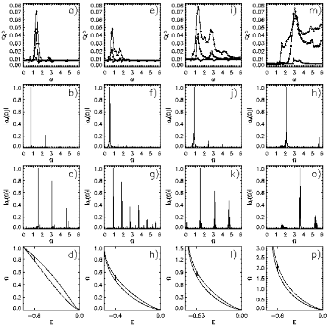
Figure 2: (a) Mean finite time Lyapunov exponent for a microcanonical sampling of 1600 orbits with initial energy $E=0.8E_{min}$ evolved in a Plummer potential for a time $t=512$ with variable frequencies ${\omega}$ and amplitudes (from bottom to top) $m_{0}=0.1$ (full circles), $m_{0}=0.2$ (empty circles) and $m_{0}=0.3$ (triangles). (b) $|a_{x}({\Omega})|$, the power spectrum of the $x$-component of the acceleration for the same orbits in the Plummer potential, evolved for a time $t=2048$ in the absence of driving. (c) $|a_{r}({\Omega})|$, the power spectrum for the radial component. (d) The analytically computed ranges of frequencies for the unperturbed Plummer sphere (solid lines), along with the peak frequencies ${\Omega}^{(1)}$ of orbits integrated in a non-pulsating potential for the initial conditions used in time-dependent integrations. (e) - (h) The same for a pulsating Dehnen potential with ${\gamma}=0$ and $E=0.8E_{min}$. (i) - (l) For a pulsating Dehnen potential with $\gamma=0.5$. (m) - (p) For a pulsating Dehnen potential with $\gamma=1.0$.

That the locations of the peaks and troughs in ${\langle}{\chi}{\rangle}$ are related to the natural frequencies of the unperturbed orbits can be seen if, in a plot of ${\langle}{\chi}{\rangle}({\omega})$, is superimposed the Fourier spectrum of the radial acceleration $|a_{r}({\Omega})|$ and/or the $x$-component $|a_{x}({\Omega})|$ for the unperturbed ensemble. Examples thereof are provided in Fig. 2, which focuses in greater detail on lower frequencies ${\leq}{\;}6.0$. Here $|a_{r}|$ is defined by analogy with eq. (3) except that the large zero frequency contribution reflecting a nonzero average $r$ has been subtracted. (The bottom row of this Figure is discussed in Section III.) There are direct correlations between $|a_{x}|$ (or $|a_{r}|$) and ${\langle}{\chi}{\rangle}$ in the sense, for example, that the spacing between successive peaks for these two quantities are often comparable in magnitude. However, it is not true that (say) peaks in $|a_{x}|$ coincide with peaks in ${\langle}{\chi}{\rangle}$. Something more complex must be going on.

To address these complications and, especially, to identify which orbits will be chaotic, it proves convenient to classify the orbits in terms of properties of their Fourier spectra. Here the most obvious tack is to determine the value of the ‘peak’ frequency ${\Omega}^{(1)}$ for each orbit, i.e., the value of ${\Omega}$ for which its $|x({\Omega})|$ (and, by symmetry, $|y({\Omega})|$ and $|z({\Omega})|$) is maximised, and to look for correlations between ${\Omega}^{(1)}$ and the finite time Lyapunov exponent ${\chi}$ for the orbit.

Far from the resonant regions, at both higher and lower frequencies, all the orbits are regular, with small values of ${\chi}$ and peak frequencies ${\Omega}^{(1)}$ relatively close to the peak frequency ${\Omega}^{(1)}_{0}$ associated with an ${\omega}=0$ orbit with the same initial condition. Closer, however, to the resonance one sees the onset of chaos, in which some of these regular orbits undergo a significant change in the form of their spectra.

Consider, for example the observed behaviour of orbits in a given ensemble as the driving frequency ${\omega}$ is slowly increased from zero to higher frequencies. The introduction of a small but nonzero ${\omega}$ alters slightly the peak frequency in the Fourier spectra $|x({\Omega})|$, but all the orbits still remain regular. Nevertheless, the spectra do become more complicated, typically acquiring additional power at one or more lower frequencies.

For sufficiently small ${\omega}$ no significant resonant couplings are triggered. However, there is an abrupt onset of chaos when ${\omega}$ becomes sufficiently large that, for some of the orbits, one or more of these new lower frequencies acquires more power than what had been the higher peak frequency ${\Omega}^{(1)}$. At this stage, resonant couplings become important and the orbits divide generically into three different populations: Population I regular orbits, which behave much the same as they did at lower driving frequencies ${\omega}$; Population II chaotic orbits, where the peak frequency ${\Omega}^{(1)}$ in the Fourier spectrum is close in value to half the driving frequency; and Population III chaotic orbits, where ${\Omega}^{(1)}$ is substantially lower and tends to drift in time.

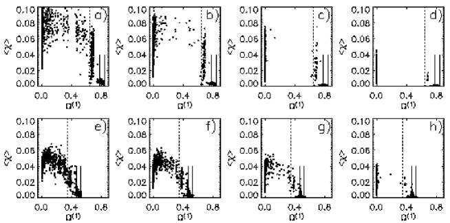
Figure 3: Finite time Lyapunov exponents as a function of peak frequency ${\Omega}^{(1)}$ for Population I (${\Omega}^{(1)}>{\omega}/2$), Population II (${\Omega}^{(1)}{\;}{\approx}{\;}{\omega}/2$), and Population III (${\Omega}^{(1)}<{\omega}/2$) orbits, generated from a microcanonical sampling of 1600 initial conditions with $E=0.8E_{min}$, evolved in a pulsating Plummer potential with ${\omega}=1.3$ and $m_{0}=0.2$ for times (a) $t=1024$, (b) $t=2048$, (c) $t=4096$ and (d) $t=8192$. The dashed vertical line corresponds to ${\omega}/2$. The vertical solid lines show the range of frequencies in the non-pulsating model. The solid vertical lines delimit the range of unperturbed peak frequencies. (e) - (h). The same for a pulsating ${\gamma}=0$ Dehnen potential with ${\omega}=0.7$, $m_{0}=0.2$, and $E=0.8E_{min}$.

Examples of this behaviour for the Plummer and ${\gamma}=0$ Dehnen potentials are provided in Fig. 3, which exhibit scatter plots of finite time Lyapunov exponent and peak frequency ${\Omega}^{(1)}$ at four times, $t=1024$, $2048$, $4096$, and $8192$.

The Population I orbits are clearly regular. Plots of the Fourier spectra for spatial coordinates and velocities exhibit sharply defined peaks and the computation of a finite time Lyapunov exponent ${\chi}(t)$ results in a uniform decay of the form expected (see, e.g., Bennetin, Galgani & Strelcyn 1976) for regular orbits. It is, for example, evident from Fig. 3 that the typical ${\chi}$ for orbits with ${\Omega}^{(1)}>{\omega}/2$ decreases as time passes. Equally clearly, the Population II and III orbits are chaotic: Their Fourier spectra are broader band, and the finite time Lyapunov exponent ${\chi}(t)$’s, typically substantially larger in magnitude, do not decay towards zero systematically.

When ${\omega}$ is nonzero, energy is (almost) never conserved since the potential is time-dependent. However, the form of the variations in energy is different for the three different orbit populations. Regular Population I orbits show completely periodic oscillations in energy, the Fourier spectra of $E(t)$ being excedingly simple and regular. For chaotic Population II orbits, changes in energy are again bounded and are again nearly oscillatory, although occasional ‘glitches’ are observed that break near-periodicity. The Fourier spectra are more complex than for the regular orbits. However, they typically assume forms which one is wont to associate with nonconserved phase space coordinates for a ‘sticky’ near-regular orbit in a time-independent potential. For the Population III chaotic orbits, the behaviour is very different. In this case, the time-dependence of the energy is far from periodic and the spectrum looks manifestly chaotic. For these orbits, the energy typically exhibits large secular variations, drifting to significantly larger or smaller values.

The distinction between regular and chaotic orbits appears to be absolute. If an initial condition corresponding to a regular orbit is integrated even for a very long time, the orbit will remain regular, with small ${\chi}$, sharply peaked Fourier spectra, and phase space coordinates confined to the same small region. By contrast, the distinction between the two types of chaotic orbits is not absolute. It appears that, if one integrates long enough – in some cases a time $t{\;}{\gg}{\;}100000$ may be required! – many (if not all) Population II orbits originally trapped near the initial regular region escape to become Population III orbits. The possibility of such transitions suggests strongly that the boundary between Populations II and III corresponds to an entropy barrier, i.e., a leaky phase space barrier through which escape is possible but which requires an orbit to ‘find a small gap’.

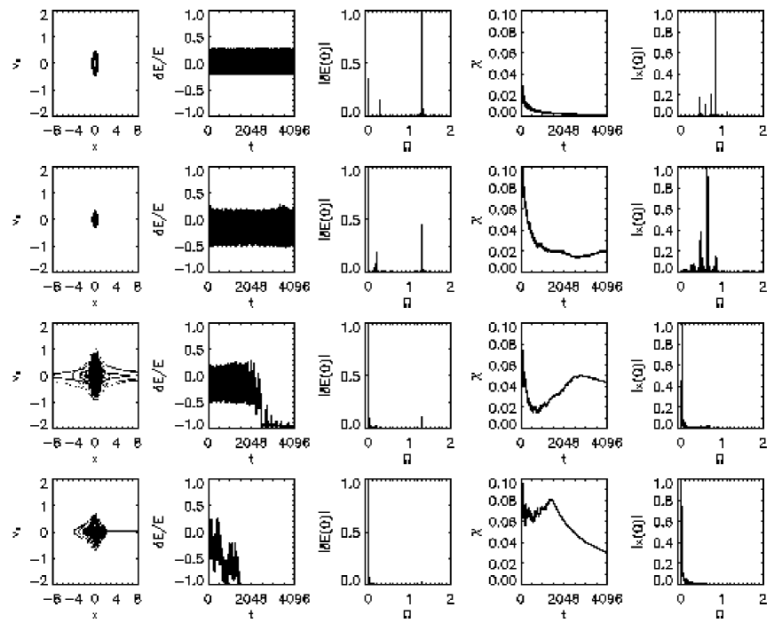
Figure 4: Top row: The phase space trajectory of a typical Population I radial orbit evolved in a pulsating Plummer potential with $E=-0.8$, $m_{0}=0.2$ and $\omega=1.3$, along with the relative energy oscillations, ${\delta}E(t)/E$, the power spectrum $|{\delta}E(\omega)|$, the finite time Lyapunov ${\chi}$ computed for times $T{\;}{\leq}{\;}t$, and the power spectrum, $|x({\Omega})|$. Second row: The same for a typical weakly chaotic orbit which remains Population II for $t<4096$. Third row: Another chaotic orbit which transforms from Population II to Population III near $t=2048$. Fourth row: A typical wildly chaotic Population III orbit.

Examples of the aforementioned behaviour are illustrated in Fig. 4, which was constructed for representative orbits in a pulsed Plummer potential. Here the left hand columns exhibits the phase space coordinates $x$ and $v_{x}$ of four representative orbits, each recorded at intervals ${\delta}t=1.0$. The second column exhibits the mean shift in energy, ${\delta}E/E$, where $\delta E\equiv E(t)-E(0)$, as a function of time, and the third column exhibits the Fourier transform of the resulting time series The fourth column exhibits the Lyapunov exponent ${\chi}$, computed for times ${\leq}{\;}t$, and the final column exhibits the power spectrum $|x({\Omega})|$.

The top row corresponds to a regular Population I orbit. The second row corresponds to an orbit which remains Population II for a time $t=4096$. The third row exhibits an orbit which transforms from Population II to Population III near $t=2048$. If the orbital integration for this orbit had been terminated at an earlier time, say $t=2048$, the points at large $x$ observed in the leftmost panel of the second row would be absent and the power spectrum $|x({\Omega})|$ would have substantially less power at very low frequencies. The fourth row exhibits a typical Population III orbit. The fact that, for the fourth orbit, ${\chi}$ decreases systematically at late times and that most of the power in $x$ is at very low frequencies manifests the fact that the orbit has been ejected to very large radii, where the dynamical time is very long and typical Lyapunov exponents for chaotic orbits are very small.

Chaotic and regular initial conditions appear to occupy distinctly different phase space regions. However, the two different types of chaotic initial conditions are not so separated: the experiments performed hitherto are consistent with the interpretation that, arbitrarily close to every Population II initial condition, there is a Population III initial condition. This suggests strongly that the entropy barriers dividing the two orbit types may be fractal, exhibiting a structure analogous topologically to cantori in time-independent Hamiltonian systems (see, e.g., Mather 1982).

On the basis of these observations, it appears reasonable to term Population II orbits as ‘sticky’ chaotic orbits which, like sticky orbits in time-independent systems (Contopoulos 1971), are trapped near regular regions; and, by contrast, to term Population III orbits as ‘wildly’ chaotic orbits, which exhibit substantial diffusion in energy space.

In any event, as the driving frequency increases, the ensemble eventually moves out of the resonance region and all (or almost all) the orbits again become regular. If, however, the amplitude of the driving is sufficiently large, other, higher frequency resonance regions also exist, in which, once again, one observes a coexistence of the three orbit populations. The only difference here is that the sticky chaotic orbits may be associated with lower harmonics of the driving frequency, such as ${\omega}/4$ and ${\omega}/6$. Eventually, however, when the driving frequency becomes too large, the chaotic orbits disappear for good and the effects of the time-dependence ‘turn off’ as the peak frequencies ${\Omega}^{(1)}$ associated with the regular orbits again approach their original values ${\Omega}^{(1)}_{0}.$

3 THE ROLE OF RESONANCES

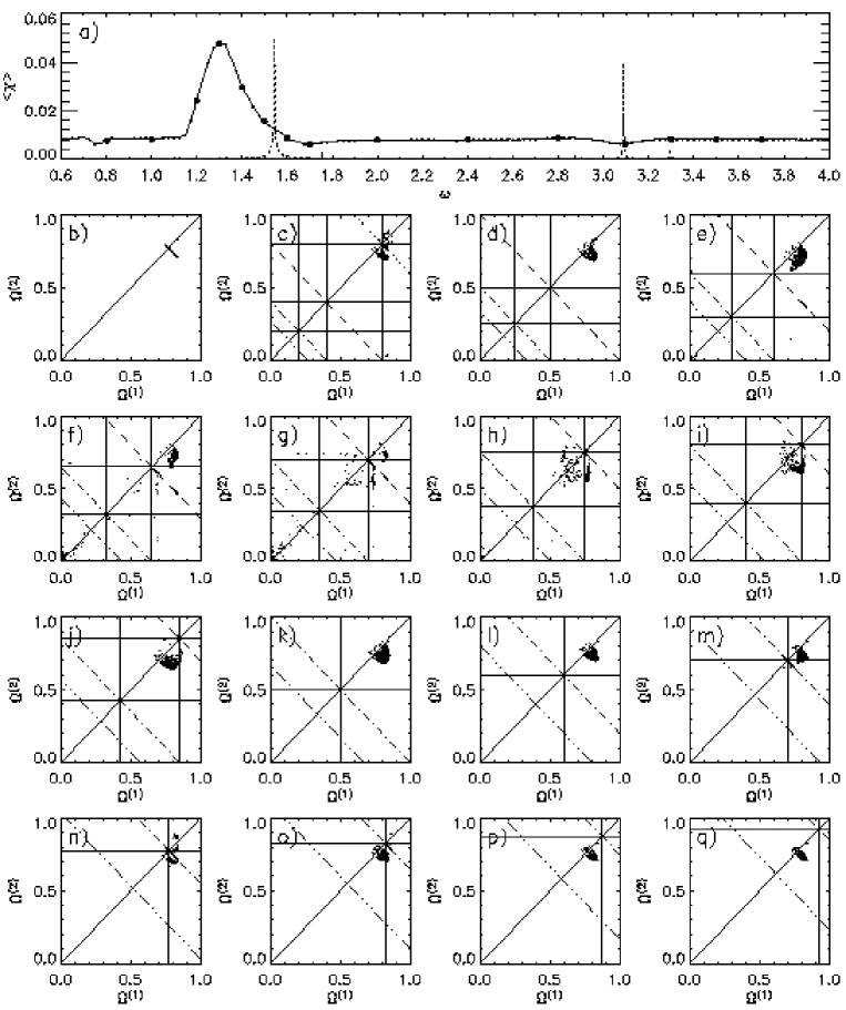
Figure 5: (a) Mean Lyapunov exponents for a microcanonical sampling of 800 orbits with initial energy $E=0.8E_{min}$, evolved in a pulsating Plummer potential with $m_{0}=0.2$ for a time $t=2048$. The power spectrum $|r({\Omega})|$ is over-plotted with dashed lines. Heavy dots correspond to panels (c) - (q), from left to right respectively. (b) A scatter plot in frequency space, exhibiting the two frequencies $\Omega^{(1)}$ and $\Omega^{(2)}$ for which, in the absence of any driving, $|x({\Omega})|$ has the most power. (c) - (q) The same for the pulsating Plummer potential with $\omega=0.8,1.0,1.2,1.3,1.4,1.5,1.6,1.7,2.0,2.4,2.8,3.1,3.3,3.5,$ and $3.7$ respectively. The thick diagonal solid line represents ${\Omega}^{(1)}={\Omega}^{(2)}$. Vertical and horizontal thin solid lines correspond to the driving frequency ${\omega}$, ${\omega}/2$, and ${\omega}/4$. Short-dashed lines represent, the $1:1$ resonance, long dashes the $2:1$ resonance, dot-dashed lines the $4:1$ resonances, and triple-dot-dashed lines the $6:1$ resonance.

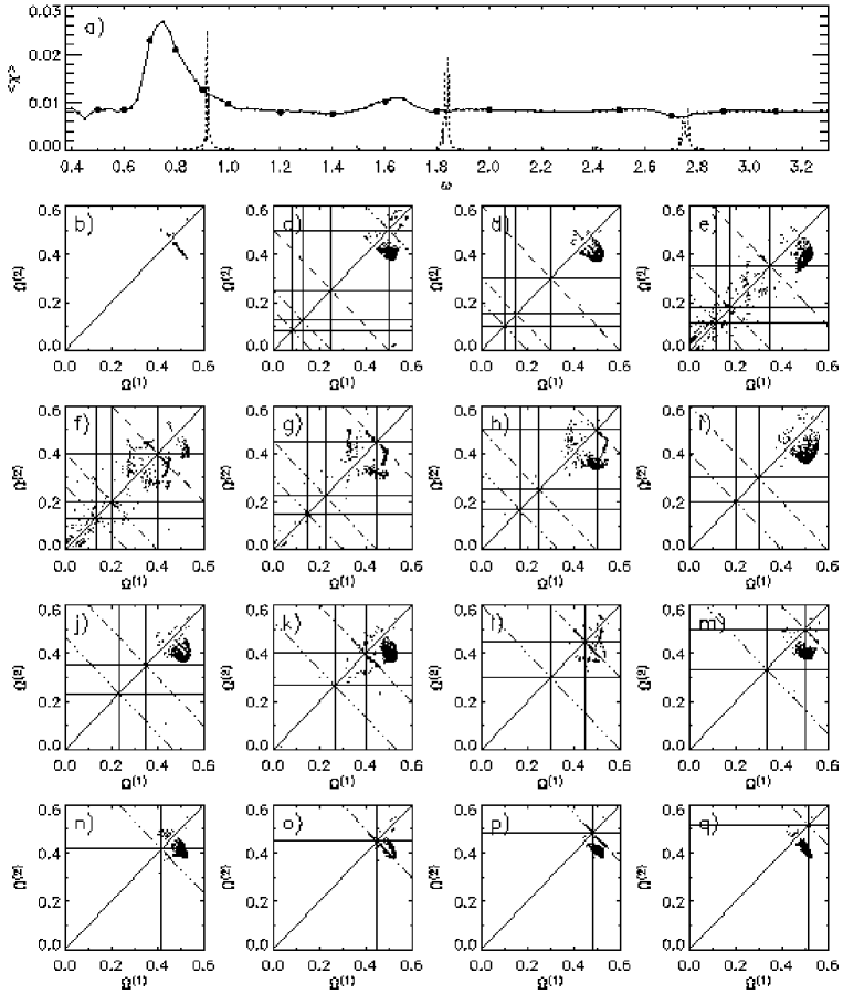
Figure 6: The same as Fig. 5, albeit for orbits with initial energy $E=0.8E_{min}$, evolved in a pulsating ${\gamma}=0$ Dehnen potential.

To better understand the role of resonant couplings, it is useful to analyse the orbital structure in frequency space by identifying for individual orbits the two frequencies in the Fourier spectra, ${\Omega}^{(1)}$ and ${\Omega}^{(2)}$, which contain the most power. Distinctive patterns relating these frequencies to one another and to the driving frequency ${\omega}$ can make the resonant nature of the dynamics apparent. In particular, orbits locked in a $n:1$ resonance between the natural frequencies and the driving frequency lie along the line ${\Omega}^{(2)}=2\omega/n-{\Omega}^{(1)}$. The results for two typical orbit ensembles, one each in the Plummer and ${\gamma}=0$ Dehnen potentials, are provided in Figs. 5 and 6, which exhibit the peak frequencies generated from $|x({\Omega})|$.

As is illustrated in the bottom row of Fig. 2, for any given energy the peak frequencies of orbits in the unperturbed Plummer and Dehnen potentials, ${\Omega}^{(1)}_{0}$, occupy only a small range of values. However, as the driving frequency is increased from zero, the interplay between the natural frequency and various harmonics of the driving frequency induces resonant structures. By far the most dominant is the $2:1$ resonance, which arises when half the driving frequency ${\omega}$ approaches the range of unperturbed natural frequencies. The proximity of ${\omega}/2$ to the natural frequency population causes the population, confined initially to a thin line (as in panels b of Figs. 5 and 6) to stretch within the confines of the unperturbed range. Eventually, however, if the amplitude of the driving is sufficiently large, which for the potentials here requires $m_{0}{\;}{\ga}{\;}0.2$, there is an onset of chaos for ${\Omega}^{(1)}-{\omega}/2{\;}{\la}{\;}m_{0}$.

Such a criterion clearly makes sense: If the amplitude of the driving is strong enough to ‘wiggle’ the frequencies to values sufficiently close to the harmonic of ${\omega}$, frequency overlap occurs and a chaotic resonance is triggered. This finding thus corroborates the expectation that chaos arises from an overlap between fundamental frequencies of the unperturbed system and harmonics of the driving frequency.

If, the Fourier spectra $|x({\Omega})|$ and $|r({\Omega})|$ are overlaid with a plot of mean values ${\langle}{\chi}{\rangle}$ as a function of ${\omega}$, one notices that the spacings between peaks are identical. To appreciate the significance of this fact, one must, however, understand the connection between $|x({\Omega})|$ and $|r({\Omega})|$. As is evident from the second and fourth rows of Fig. 2, if one denotes by ${\Omega}_{0}$ the value of ${\Omega}$ associated with the lowest frequency peaks in $|x({\Omega})|$ and $|a_{x}({\Omega})|$, the remaining higher frequency peaks represent odd harmonics $3{\Omega}_{0}$, $5{\Omega}_{0}$, . . . . By contrast, the dominant frequency for $|r({\Omega})|$ and $|a_{r}({\Omega})|$ is $2{\Omega}_{0}$ and the higher frequency peaks correspond to multiples thereof. This means that $2m:1$ resonances between the driving frequency and the natural frequencies of motion in the $x$-direction (and, by symmetry, the $y$- and $z$-directions) correspond to $m:1$ resonances between ${\omega}$ and the natural radial frequencies. The spacing between successive peaks in both the $x$- and $r$-coordinates is $2{\Omega}_{0}$. This is accurate at least to within half the width of the unperturbed natural frequency range to which ${\Omega}_{0}$ belongs.

Understanding the onset of chaos, as probed by the mean Lyapunov exponent ${\langle}{\chi}{\rangle}$, as a chaotic resonance between the driving frequency and the range of natural frequencies for the ensemble provides a clear explanation of why the spacing between peaks in ${\langle}{\chi}{\rangle}$ as a function of ${\omega}$ are the same as the spacing between peaks in $|x({\Omega})|$ and $|r({\Omega})|$ as a function of ${\Omega}$. Interestingly, however, for lower amplitude pulsations, generally $m_{0}{\;}{\la}{\;}0.2$, some peaks in $|r({\Omega})|$ correspond almost exactly to minima in the amount of chaos although, for larger amplitude, these minima are overtaken by nearby maxima which emerge as chaos becomes more prevalent. If orbits are pulsed with sufficiently small amplitude at a frequency that is a harmonic of its natural frequency, the pulsation will make them more stable (in the sense that ${\chi}(t)$ converges faster towards zero than for unperturbed orbits), whereas increasing the amplitude of pulsations eventually renders them chaotic.

The resonance structure of the Plummer potential and all the Dehnen potentials, both cuspy and cuspless, are qualitatively very similar. Resonances occur whenever the driving frequency ${\omega}$ is close to a harmonic of the unperturbed natural frequency range, the locations of which vary from model to model. Besides the dominant $2:1$ resonance, there are other resonances which cause a significant alignment of orbits along the resonance lines in frequency space, even when they do not trigger a large measure of chaotic orbits. For example, as is evident from Figs. 5 m-o and Figs. 6 k-p, both the $4:1$ and $6:1$ resonances are clearly present. Their importance and effect relative to the dominant $2:1$ resonance is commensurate to the relative power of those frequencies in $|r({\Omega})|$, which is shown in Figs. 5 a and 6 a.

4 PHYSICAL IMPLICATIONS

The analysis described hitherto has focused on distinctions between regular and chaotic orbits and on determining which resonances are responsible for regulating the properties of different orbits. Attention now focuses on statistical properties of orbit ensembles, and how these properties depend on the amplitude and the frequency of the driving.

Macroscopically, perhaps the most obvious measure of the efficacy of the driving is the degree to which it occasions large systematic changes in energy. In particular, one can ask when the driving causes appreciable numbers of orbits to be ejected to infinity, acquiring positive energy. The answer here is that, even if the driving is relatively low amplitude, for example $m_{0}{\;}{\sim}{\;}0.2$ or less, a sizeable fraction of the orbits can be ejected if the driving frequency is in the appropriate range. This is illustrated in Fig. 7, which focuses on orbit ensembles with initial energy $E=0.6E_{min}$ evolved in pulsed Plummer and ${\gamma}=0$ Dehnen potentials with amplitude $m_{0}=0.2$ and variable driving frequency.

In each case, two different sets of initial conditions were evolved, namely (i) a microcanonical sampling of the constant energy hypersurface (filled circles) and (ii) initial conditions corresponding to purely radial orbits which sampled uniformly the energetically accessible values of $r$ (open circles). The top panels exhibit as a function of ${\omega}$ the fraction $f_{e}$ of the orbits which have acquired positive energy by $t=4096$, the middle panels the mean change in energy at $t=4096$, and the bottom panels mean finite time Lyapunov exponents.

It is evident that there is a well-defined ‘window’ of frequencies for which ejection can occur. For both the Plummer and Dehnen models, as ${\omega}$ is increased from very small values there is an abrupt onset of ejections, with $f_{e}$ increasing from zero to its maximum value over a very short frequency interval. The ‘closing’ of the window at higher frequencies tends to be more gradual.

Overall, the frequencies which yield the largest fraction of ejected orbits and the largest changes in energy tend to correlate with those frequencies for which the mean ${\langle}{\chi}{\rangle}$ is especially large. However, this correlation is not one-to-one. For example, for a microcanonical sampling evolved in the ${\gamma}=0$ Dehnen potential the largest energy shift occurs for ${\omega}{\;}{\sim}{\;}0.8$ but ${\langle}{\chi}{\rangle}$ peaks near ${\omega}{\;}{\sim}{\;}2.5$. At least in part, such discrepancies arise as a sampling effect.

For those frequencies for which driving has the largest effect, many of the orbits have been ejected to large radii already at times $t{\;}{\ll}{\;}4096$ – this is, for example, the case in the Plummer potential for ${\omega}{\;}{\sim}{\;}1$. However, the value of the largest Lyapunov exponent scales (at least roughly) inversely with the orbital time scale $t_{D}$, so that the short time ${\chi}$ for orbits at large $r$ tends to be very small. For frequencies where large numbers of orbits have been ejected at early times, the values of ${\langle}{\chi}{\rangle}$ exhibited in panels (c) and (f) reflects an average over a short interval where orbits at relatively small $r$ have large ${\chi}$ and a (often much) longer interval where orbits at larger $r$ have much smaller ${\chi}$.

The final obvious point evidenced in Fig. 7 is that, in the resonance region, as probed both by the degree of chaos and by the typical energy shifts experienced, radial orbits tend to be more impacted by the driving than ‘generic’ orbits with the same energy. As is evident from Figs. 7 (b) and (d), outside the resonant region the microcanonical and radial ensembles behave in a fashion which is virtually identical. Inside this region, however, the radial orbits are ejected more frequently, experience larger energy shifts, and have larger finite time Lyapunov exponents. Only near the low frequency boundary of the resonance region are the effects of the driving comparable for radial and generic ensembles.

That radial orbits are impacted more strongly reflects the fact that they have significantly more power at higher frequencies than nonradial orbits, which allows for more efficient resonant couplings. An example of this extra high frequency power is provided in Fig. 8, which exhibits $|a_{x}({\Omega})|$ and $|a_{r}({\Omega})|$ for representative ensembles of unperturbed radial orbits for the same potentials and energies that were sampled microcanonically to generate Fig. 2.

As evidenced, for example, by Figs. 7 (c) and (f), for comparatively low amplitudes $m_{0}$ the degree of chaos, as probed by the mean ${\langle}{\chi}{\rangle}$, can exhibit a relatively complex dependence on ${\omega}$, although there is a relatively smooth overall envelope for ${\langle}{\chi}{\rangle}({\omega})$. However, as illustrated in Figs. 1 (a) and (b), the short-scale structure tends to ‘smooth out’ as $m_{0}$ is increased, this presumably correlating with the fact that the resonances broadened with increasing amplitude.

By contrast, as illustrated in Fig. 9, for fixed ${\omega}$, the mean ${\langle}{\chi}{\rangle}$ exhibits a comparatively smooth dependence on $m_{0}$. Once $m_{0}$ has become sufficiently large to elicit a significant response, ${\langle}{\chi}{\rangle}$ becomes a smooth, monotonically increasing function of $m_{0}$ until the amplitude becomes so large that many orbits are ejected to very large radii, where ${\chi}$ become very small. Significant also is the fact that, for weak driving, orbits tend oftentimes to lose energy and move inwards, whereas, for stronger driving, $m_{0}{\;}{\ga}{\;}0.2$, orbits tend generically to gain energy and move towards larger radii.

5 CONCLUSIONS AND EXTENSIONS

The analysis described here focused on the particularly simple case in which spherically symmetric, integrable potentials are subjected to strictly periodic perturbations of an especially simple form; and, for this reason, many of the detailed findings are no doubt nongeneric. The assumption of spherical symmetry is useful in that it limits the number of resonances that could be triggered, and the fact that the unperturbed potentials are integrable implies that all the chaos that arises must be be associated with the time-dependence. That the perturbation reflects a single large scale perturbation makes the relevant resonances especially easy to identify. And, most especially, the seemingly absolute distinction between regular and chaotic orbits no doubt reflects the strictly periodic form of the time-dependence. One knows from other examples (see, e.g., Kandrup & Drury 1998) that the introduction of a time-dependent potential that exhibits systematic secular changes can occasion transitions between regularity and chaos.

However, several of the conclusions derived from these models are likely to be robust. Most obvious is the possibility of distinguishing between orbits which, over finite time intervals, exhibit exponential sensitivity and hence deserve the appellation chaotic, and other, presumably regular, orbits that do not. Moreover, there is the fact that, as one might have expected, orbital structure and the onset of chaos can be associated with specific resonances, the identities of which could no doubt change in time were one to allow for a more complex time-dependence.

It is also apparent that chaotic orbits in a time-dependent potential need not exhibit large scale energy diffusion, at least over finite time intervals. It may be that, in generic potentials, distinctions between ‘sticky’ and ‘wildly’ chaotic orbits are less clear than is the case for the models considered here, especially since ‘sticky’ orbits appear tied to specific subharmonics of the driving frequency, which will vary for a generic time-dependence. However, it is evident that ‘chaotic’ need not necessarily imply large scale systematic changes in energy. In time-dependent systems exhibiting large amounts of chaos, mixing in energies can proceed far less efficiently than mixing in other phase space variables.

Relaxing the underlying assumptions entering into this paper could in some cases make it difficult, if not impossible, to determine precisely the resonance structure of orbits. However, there are a variety of interesting issues which can, and should, be addressed. Most obvious, perhaps, is the question of what would happen if the unperturbed integrable models considered here were replaced by nonintegrable models which admit large measures of chaotic orbits even in the absence of a time-dependence. One might, for example, expect that such systems would be even more susceptible to resonant couplings since the Fourier spectra associated with already chaotic orbits are broad band, with power spread over a continuous range of frequencies (Kandrup, Abernathy & Bradley 1995). However, it might well prove that, in some cases, adding a time-dependence actually converts chaotic orbits into regular.

It would also be of some interest to determine the sorts of resonances that are triggered when a system, integrable or otherwise, is subjected to other sorts of periodic time-dependences. For example, an analysis of galactic potentials subjected to a (near-)periodic time-dependence associated with a supermassive black hole binary shows that the orbital frequencies of the binary which trigger large changes in energy and large measures of chaotic orbits need not coincide with the frequencies for which a global time-dependence $V({\bf r},t)=V_{0}({\bf r})(1+m_{0}\sin{\omega}t)$ triggers large amounts of chaos (Kandrup, Sideris, Terzić & Bohn 2003).

And similarly, as a prolegomena to realistic self-consistent computations, it would seem important to investigate the effects of large scale variations in the amplitude and frequency of the time-dependence, for example by allowing the frequency to drift and/or allowing the amplitude to decrease. Some limited work on this issue was described in Kandrup, Vass & Sideris (2003), which considered bulk oscillations that eventually damp away and random variations in frequency modeled as colored noise. However, that work was limited in the sense that attention focused completely on bulk statistical properties of orbit ensembles, without any consideration of orbital structure.

From a more formal perspective, it would seem interesting to pursue possible analogies between phase space topologies in two-degree-of-freedom, time-independent Hamiltonian systems and $1{1\over 2}$-degree-of-freedom systems (Lichtenberg & Lieberman 1992) associated with time-dependent, spherically symmetric potentials, for example by reformulating the analysis described in this paper in the context of an ‘enlarged phase space’ that includes time and energy as additional coordinates. It is well known that, in two-degree-of-freedom time-independent systems, topological considerations preclude the existence of an Arnold web (Arnold 1964). However one expects generically that the chaotic phase space regions near regular islands will be permeated by cantori. Analogous considerations would suggest that a $1{1\over 2}$-degree-of-freedom system cannot admit an Arnold web, but that some analogue of cantori could exist.

But what might all this mean for real galaxies? Time-dependent potentials arise naturally in a variety of astronomical contexts, including long-lived (quasi-)normal modes, triggered, for example, by close encounters between galaxies (e.g., Vesperini & Weinberg 2000) and, most obviously, in the violent relaxation of a galaxy involved in a strong encounter.

The normal-mode setting, which involves relative low amplitudes, is more directly related to the computations described in this paper. Here it would appear that, as a result of the oscillations, a significant number of orbits could become chaotic, some exhibiting system drifts in energy and others ‘locked’ to a harmonic of the driving frequency. All the chaotic orbits can participate in chaotic mixing on a constant energy hypersurface. More importantly, however, the ‘wildly’ chaotic orbits can also mix in energy space, a process which could trigger a relatively slow (time scale ${\gg}\,t_{D}$) change in the density distribution. Presuming, as would seem likely (e.g., Kandrup, Sideris, Terzić & Bohn 2003) that this effect persists in strongly nonspherical systems, this effect could help drive an asymmetrically-shaped galaxy towards a more axisymmetric shape, a possibility envisioned by Merritt (1999), or, perhaps, towards some other shape that minimizes the amount of chaos (Kandrup & Siopis 2003). Moreover, to the extent that the oscillations persist for a long time, many of the ‘sticky’ orbits could become unstuck and, as such, participate in this mixing.

As evidenced in Section IV, even relatively low amplitude driving can also result in an appreciable number of stars being displaced to very large radii, and, in some cases, being expelled from the galaxy, presumably in a comparatively incoherent fashion. This suggests that, even ignoring direct galaxy-galaxy collisions, lower-amplitude galactic ‘harrassment’ could lead to the presence of a diffuse population of stars and/or gas in intergalactic space.

Violent relaxation differs in that the amplitude of the time-dependence is substantially higher (at least initially), that one would expect larger variations in the oscillation frequency over time scales ${\sim}{\;}t_{D}$ and, of course, that the time-dependence should damp systematically on a time scale not much longer than $t_{D}$. Larger amplitude typically implies broader resonances and, hence, larger numbers of chaotic orbits with larger finite time Lyapunov exponent. Indeed, given plausible assumptions it appears likely that all – or almost all – the orbits in some parts of phase space will be chaotic and, as such, available to participate in chaotic phase mixing (Kandrup, Vass & Sideris 2003). Moreover, allowing for a changing oscillation frequency need not decrease the abundance of chaos. Indeed, in some cases allowing for variations in frequency modeled as coloured noise with a nonzero autocorrelation time actually increases the relative fraction of orbits that are chaotic (Kandrup, Vass & Sideris 2003).

The only question is whether a sufficiently large fraction of the chaotic orbits will exhibit secular variations in energy, thus facilitating mixing in energy space. The answer to this question must of course be addressed in the context of honest self-consistent simulations. However, it would seem reasonable to expect that variations in the frequency and the amplitude of the driving might make the frequency ‘locking’ of sticky chaotic orbits more difficult to maintain, so that most of the chaotic orbits will exhibit the drifts in energy required to drive violent relaxation.

Figure 1: (a) Mean finite time Lyapunov exponent ${\langle}{\chi}{\rangle}$ for a microcanonical sampling of 1600 orbits with initial energy $E=-0.5$ evolved in a Plummer potential subjected to periodic driving with variable frequency ${\omega}$ with amplitudes (from bottom to top) $m_{0}=0.125$, $0.25$, and $0.5$. (b) The same for an ensemble evolved in the ${\gamma}=1$ Dehnen potential. (c) The power spectrum of the acceleration $|a_{x}({\Omega})|$ for the same orbits in the Plummer potential, evolved in the absence of driving. (d) The same for orbits in the ${\gamma}=1$ Dehnen potential with $E=-0.5E$. Each orbit was evolved for a time $t=512$.

Figure 7: (a) Fraction of orbits with initial energy $E=0.6E_{min}$, evolved in a pulsating Plummer potential with $m_{0}=0.2$ and variable driving frequency that have been ejected, i.e., acquired positive energy, by time $t=4096$. Filled circles represent initial conditions sampling a microcanonical distribution. Open circles sample a distribution corresponding to purely radial orbits. Each point represents $400$ orbits. (b) Mean relative change in energy for the ensemble after $t=4096$. (c) Mean finite time Lyapunov exponent for the ensemble. (d) - (f) The same for an ensemble with $E=0.6E_{min}$, evolved in a pulsating ${\gamma}=0$ Dehnen potential.

Figure 8: (a) $|a_{x}({\Omega})|$, the power spectrum of the $x$-component of the acceleration for a representative ensemble of radial orbits with energy $E=0.8E_{min}$ evolved in the Plummer potential. absence of driving. (b) $|a_{r}({\Omega})|$, the power spectrum for the same orbits. (c) - (d) The same for a pulsating Dehnen potential with ${\gamma}=0$ and $E=0.8E_{min}$. (e) - (f) For a pulsating Dehnen potential with $\gamma=0.5$. (g) - (h) For a pulsating Dehnen potential with $\gamma=1.0$.

Figure 9: (a) Mean fractional energy shift for a microcanonical sampling of 1600 orbits with initial energy $E=0.8E_{min}$ evolved in a pulsating Plummer potential with frequency ${\omega}=1.5$ and variable amplitude $m_{0}$ for a time $t=4096$. (b) The mean finite time Lyapunov exponents computed for the same orbits. (c) and (d) The same for a pulsating ${\gamma}=0.0$ Dehnen potential with $E=0.8E_{min}$ and ${\omega}=0.8$. (e) and (f) The same for a pulsating ${\gamma}=0.5$ Dehnen potential with $E=0.8E_{min}$ and ${\omega}=1.2$.

References

- [1] Arnold, V. I. 1964, Russ. Math. Surveys 18, 85
- [2] Bennetin, G., Galgani, L., Strelcyn, J. M. 1976, Phys. Rev. A 14, 2338
- [3] Contopoulos, G. 1971, AJ 76, 147
- [4] Dehnen, W. 1993, MNRAS 265, 250
- [5] Gluckstern, R. L. 1994, Phys. Rev. Lett. 73, 1247
- [6] Kandrup, H. E. 2003, Springer Lecture Notes in Physics, in press (astro-ph/0212031)
- [7] Kandrup, H. E., Abernathy, R. A., Bradley, B. O. 1995, Phys. Rev. E 51, 5287
- [8] Kandrup, H. E., Drury, J. 1998, Ann. N. Y. Acad. Sci., 867, 306
- [9] Kandrup, H. E., Mahon, M. E., Smith, H. 1993, A&A, 271, 440
- [10] Kandrup, H. E., Sideris, I. V., Terzić, B., Bohn, C. L. 2003 ApJ, 597, 111
- [11] Kandrup, H. E., Siopis, C. 2003, MNRAS, 345, 727
- [12] Kandrup, H. E., Vass, I. M., Sideris, I. V. 2003, MNRAS, 341, 927
- [13] Lichtenberg, A. J., Lieberman, M. A. 1992, Regular and Chaotic Dynamics, Springer, Berlin
- [14] Lynden-Bell, D. 1967, MNRAS, 1361, 101
- [15] Mather, J. N. 1982, Topology 21, 45
- [16] Merritt, D. 1999, PASP, 111, 129
- [17] Matthews, J. Walker, R. L. 1970, Mathematical Methods of Physics, Benjamin, Menlo Park
- [18] Quinn, P. J., Zurek, W. H. 1988, ApJ, 331, 1
- [19] Vesperini, E., Weinberg, M. D., 2000, ApJ, 534, 598