String Imprints from a Pre-inflationary Era

Abstract

We derive the equations governing the dynamics of cosmic strings in a flat anisotropic universe of Bianchi type I and study the evolution of simple cosmic string loop solutions. We show that the anisotropy of the background can have a characteristic effect in the loop motion. We discuss some cosmological consequences of these findings and, by extrapolating our results to cosmic string networks, we comment on their ability to survive an inflationary epoch, and hence be a possible fossil remnant (still visible today) of an anisotropic phase in the very early universe.

I Introduction

Cosmological inflation Guth (1981); Albrecht and Steinhardt (1982); Linde (1983, 1994) is a fairly simple paradigm whose main virtue lies in its ability to solve a number of the problems of standard cosmology, in particular those related to initial conditions. Even though it has proven difficult to find a single inflationary model that is both (1) well motivated in terms of a more fundamental theory and (2) in complete agreement with observations, the inflationary paradigm is broad enough to allow simple toy models to be in quite good agreement with observational results Bennett et al. (2003); Peiris et al. (2003).

Roughly speaking, the way inflation solves these initial condition problems is by erasing the previously existing conditions and effectively ‘re-starting’ the universe to a fairly simple state. Depending on one’s point of view, this can be seen either as blessing or as a curse. The reason for the latter view is that if inflation is very effective (in practice, if it acts long enough) then we have essentially no hope of probing the physics of a pre-inflationary epoch—see Barrow and Liddle (1997); Liddle (1999) for enlightening discussions of these issues.

Fortunately there can be relics left behind after inflation. One possible example is topological defects Vilenkin and Shellard (1994), formed at phase transitions either before or during inflation Contaldi et al. (1999); Battye and Weller (2000); Avelino et al. (1999a). The inflationary epoch will clearly have the effect of diluting the defect density, and push the network outside the horizon, freezing it in co-moving coordinates in the process. However, once the inflationary epoch ends the subsequent evolution of the defects is necessarily such as to make them come back inside the horizon Avelino et al. (1999a); Avelino and Martins (2000a).

In previous work Avelino and Martins (2000a), we have discussed a specific example of this behavior. We have considered a domain wall network produced during an anisotropic phase in the very early universe (see Bunn et al. (1996) for constraints on the present level of anisotropy), and shown that in plausible circumstances it could still be present today and have within it some imprints of the early anisotropic phase. In the present work, we discuss the analogous scenario for cosmic string networks. Just as in the domain wall case, we expect such a network to retain some imprints of such an early anisotropic phase, since it is well known Martins and Shellard (1996, 2002); Moore et al. (2002) that only if it is in a relativistic, linear scaling regime can such a network erase the traces of its former conditions. We shall start by discussing cosmic string evolution in a flat, anisotropic (Bianchi type I) universe in Sect. II, and the evolution of the background in Sect. III. We then study numerically the evolution of cosmic string loops in Sect. IV, emphasizing the differences with respect to the standard (isotropic case). Finally in Sect. V we comment on the implications of our results to the evolution of cosmic string networks as a whole, and we summarize our results in Sect. VI. Throughout the paper we shall work in units where $c=\hbar=1$.

II Cosmic string evolution

Let us consider the evolution of a cosmic string in a flat anisotropic universe of Bianchi type I, with line element:

$$ds^{2}=dt^{2}-X^{2}(t)x^{2}-Y^{2}(t)dy^{2}-Z^{2}(t)dz^{2}\,.$$ (1)

Here $X(t)$,$Y(t)$ and $Z(t)$ are the cosmological expansion factors in the $x$, $y$ and $z$ directions respectively, and $t$ is physical time. We also define $A\equiv{\dot{X}}/X$, $B\equiv{\dot{Y}}/Y$ and $C\equiv{\dot{Z}}/Z$ where the dot represents a derivative with respect to physical time t.

In the limit where the curvature radius of a cosmic string is much larger than its thickness, we can describe it as a one-dimensional object so that its world history can be represented by a two-dimensional surface in space-time (the string world-sheet)

$$x^{\nu}=x^{\nu}(\zeta^{a})\,;\qquad a=0,1\,;\quad\nu=0,1,2,3$$ (2)

obeying the usual Goto-Nambu action

$$S=-\mu\int{\sqrt{-\gamma}}d^{2}\zeta\,,$$ (3)

where $\mu$ is the string mass per unit length, $\gamma_{ab}$ is the two-dimensional world-sheet metric and $\gamma={\rm det}(\gamma_{ab})$. Let us also define

$${\bf{\dot{x}}}^{2}\equiv g_{\alpha\beta}{\dot{x}}^{\alpha}{\dot{x}}^{\beta}=1-X^{2}{\dot{x}}^{2}-Y^{2}{\dot{y}}^{2}-Z^{2}{\dot{z}}^{2}\,$$ (4)

and

$${\bf x^{\prime}}^{2}\equiv g_{\alpha\beta}x^{\prime\alpha}x^{\prime\beta}=-X^{2}x^{\prime 2}-Y^{2}y^{\prime 2}-Z^{2}z^{\prime 2}\,,$$ (5)

so that $\gamma={\bf{\dot{x}}}^{2}{\bf x^{\prime}}^{2}$ (using ${\bf{\dot{x}}}\cdot{\bf x^{\prime}}\equiv g_{\alpha\beta}x^{\prime\alpha}{\dot{x}}^{\beta}=0$ as a gauge condition).

If we choose $\zeta^{0}=t$ and define $\zeta\equiv\zeta^{1}$ then the string equation of motion is given by Vilenkin and Shellard (1994)

$$\frac{\partial}{\partial t}\left(\frac{{\dot{x}}^{\mu}{\bf x^{\prime}}^{2}}{\sqrt{-\gamma}}\right)+\frac{\partial}{\partial\zeta}\left(\frac{x^{\prime\mu}{\bf{\dot{x}}}^{2}}{\sqrt{-\gamma}}\right)+\frac{1}{\sqrt{-\gamma}}\Gamma^{\mu}_{\nu\sigma}({\bf x^{\prime}}^{2}{\dot{x}}^{\nu}{\dot{x}}^{\sigma}+{\bf{\dot{x}}}^{2}x^{\prime\nu}x^{\prime\sigma})=0\,.$$ (6)

From the time component we can obtain

$${\dot{\epsilon}}+\epsilon\left[AX^{2}\left({\dot{x}}^{2}-\frac{x^{\prime 2}}{\epsilon^{2}}\right)+BY^{2}\left({\dot{y}}^{2}-\frac{y^{\prime 2}}{\epsilon^{2}}\right)+CZ^{2}\left({\dot{z}}^{2}-\frac{z^{\prime 2}}{\epsilon^{2}}\right)\right]=0\,$$ (7)

where we have made the further definition

$$\epsilon\equiv{\sqrt{-{\bf x^{\prime}}^{2}/{\bf{\dot{x}}}^{2}}}={\bf x^{\prime}}^{2}/{\sqrt{-\gamma}={\sqrt{-\gamma}}/{\bf{\dot{x}}}^{2}}\,.$$ (8)

On the other hand, the $x$ component gives

$${\ddot{x}}+\left(\frac{\dot{\epsilon}}{\epsilon}+2A\right){\dot{x}}+\frac{1}{\epsilon}\left(\frac{x^{\prime}}{\epsilon}\right)^{\prime}=0\,,$$ (9)

and analogous equations obviously hold for the $y$ and $z$ components. One can show that in the limit of an isotropic universe these equations reduce to the usual form Vilenkin and Shellard (1994).

III Background evolution

The time component of the Einstein equations in a flat anisotropic universe of Bianchi type I is given by

$${\dot{\theta}}+A^{2}+B^{2}+C^{2}=-{1\over 2}k(\rho+3p),$$ (10)

while the spatial components give

$${\dot{A}}+\theta A={\dot{B}}+\theta B={\dot{C}}+\theta C={1\over 2}k(\rho-p),$$ (11)

and we have made the following auxiliary definitions

$$A=\frac{{\dot{X}}}{X}\,,\qquad B=\frac{{\dot{Y}}}{Y}\,,\qquad C=\frac{{\dot{Z}}}{Z}\,,$$ (12)

$$\theta=A+B+C\,,$$ (13)

and $k=8\pi G$. It is also useful to combine equations (10-11) to obtain

$$AB+BC+CA=k\rho\,.$$ (14)

In the following discussion we will make the simplification that $Z(t)=X(t)$ (and therefore $C=A$) and consider the dynamics of the universe during an inflationary phase with $\rho=-p=const$. In this case $H^{2}\equiv k\rho/3=const.$ and the Einstein field equations (10-14) imply that

$${\dot{A}}+{3\over 2}(A^{2}-H^{2})=0,$$ (15)

while $B$ can be found from the suggestive relation

$$\frac{B}{A}=\frac{1}{2}\left(\frac{3H^{2}}{A^{2}}-1\right).$$ (16)

Equation (15) has two solutions, depending on the initial conditions. If $A_{i}<H$, then $A$ is the smallest of the two dimensions and the shape of spatial hyper-surfaces is similar to that of a rugby ball. Then the solution is

$$\frac{A}{H}=\tanh\left[\frac{3}{2}H(t-t_{i})+\tanh^{-1}\left(\frac{A_{i}}{H}\right)\right],$$ (17)

with $A_{i}=A(t_{i})$. On the other hand, if $A_{i}>H$, then $A$ is the larger of the dimensions and the shape of spatial hyper-surfaces is similar to that of a pumpkin. In that case the solution is

$$\frac{A}{H}=\coth\left[\frac{3}{2}H(t-t_{i})+\coth^{-1}\left(\frac{A_{i}}{H}\right)\right]\,.$$ (18)

Note that in both cases the ratio $A/H$ tends to unity exponentially fast, and hence the same happens with the ratio $B/A$. In other words, inflation tends to make the universe more isotropic, as expected. An easy way to see this is to consider the ratio of the two different dimensions—let us call it $D=B/A$—and to study its evolution equation. One easily finds

$${\dot{D}}=\sqrt{6}H\left(D+\frac{1}{2}\right)^{1/2}(1-D),$$ (19)

which has an obvious attractor at $D=1$.

Note that even though we have so far assumed (for simplicity) that $p=-\rho$, the same analysis can be carried out for an inflating universe with $p=w\rho$ with $w\neq-1$ by numerically solving the conservation equation

$${\dot{\rho}}+\theta(\rho+p)=0,$$ (20)

together with equations (11-14). Indeed, the more general case will be relevant for what follows Avelino and Martins (2000a).

IV Numerical Simulations

Let us start by considering the simple case of the evolution of an initially static circular cosmic string loop. Its trajectory in the $z=0$ plane can be written as

$${\bf x}(t,\theta)=q(t,\theta)\left(\sin\theta,\cos\theta,0\right),$$ (21)

where $t$ is again physical time. Let us define

$$r_{x}(t,\theta)=Xq(t,\theta)\,,\qquad r_{y}(t,\theta)=Yq(t,\theta)\,,$$ (22)

$$v_{x}(t,\theta)=X\frac{dq(t,\theta)}{dt}\,,\qquad v_{y}(t,\theta)=X\frac{dq(t,\theta)}{dt}\,.$$ (23)

In the particular case of a spherical loop in a homogeneous and isotropic universe $q$ is independent of $\theta$, and hence the evolution equations become Martins and Shellard (1996)

$$\frac{dv}{dt}=(1-v^{2})\left(-\frac{1}{aq}-2Hv\right)\,,$$ (24)

with $H=A=B=C$, $a=X=Y=Z$ and $v=v_{x}=v_{y}$. In what follows we shall numerically study the evolution of initially static circular loops in a flat anisotropic universe, and discuss the dependence of the results on the background evolution.

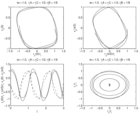
Figure 1: Phase space diagrams (in both the $x$ and the $y$ directions) and time evolution for the loop sizes and velocities, for the case of a relatively ‘small’ loop. In the bottom left panel the solid lines represent the loop radii and the dashed lines represent the loop velocities. See the main text for the definitions of the various quantities.

In Fig. 1 we plot the phase space diagrams in both directions, $(r_{x}(0)/r_{i},v_{x}(0))$ and $(r_{y}(\pi/2)/r_{i},v_{y}(\pi/2))$, and the corresponding time evolution of the loop sizes and velocities ($r_{x}(0)/r_{i}$, $r_{y}(\pi/2)/r_{i}$, $v_{x}(0)$ and $v_{y}(\pi/2)$), of an initially static circular loop with $r_{i}=r_{x}(0)=r_{y}(0)=0.5/A=0.125/B$ for the $w=-1$ case. We clearly see that the motion of the loop in an anisotropic universe is no longer periodic, with the anisotropy in the background evolution clearly affecting the loop motion. This effect only disappears for very small loops ($r_{i}H\ll 1)$.

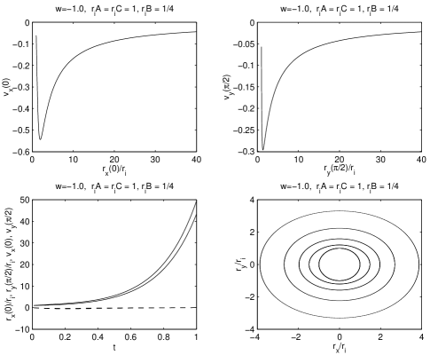
Figure 2: Same as Fig. 1, but for a larger loop (with twice the size).

Fig. 2 shows analogous plots but now a larger loop (with twice the size) is considered. In this case the loop dynamics is dominated by the strong damping caused by the exponential expansion, which drives the loop velocity towards zero and freezes the loop in comoving coordinates.

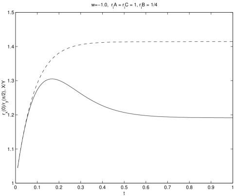
Figure 3: Evolution of the shape of the loop, parametrized by $r_{x}(0)/r_{y}(\pi/2)$ (solid line), and of the ratio between the scale factors in the $x$ and $y$ directions $(X/Y)$ (dashed line) with physical time, for the larger loop of Fig. 2. Here, we assume that $X(0)=Y(0)$.

The final shape of loop will be highly asymmetric (see Fig. 3 for the case of the loop shown in Fig. 2). The degree of asymmetry will depend both on the initial size of the loop and on the asymptotic value of $X/Y$. The asymptotic values of the degree of asymmetry (parametrized by $r_{x}(0)/r_{x}(\pi/2)$) and $X/Y$ will be equal for very large loops. For smaller loops the final degree of asymmetry will be smaller, being bound from above by $X/Y$. It is also straightforward to show Avelino and Martins (2000a) that the smaller $w$ is the faster the universe becomes isotropic and the smaller is the asymptotic value of $X/Y$.

Note that although we only study simple loop solutions our main results are also expected to hold for the more realistic loops produced by a cosmic string network.

V Consequences for Cosmic String Networks

From the results of the previous section and the basic features of the standard scenario of cosmic string evolution Martins and Shellard (1996, 2002); Moore et al. (2002) a number of interesting conclusions can be drawn concerning the evolution of full cosmic string networks in anisotropic universes.

Firstly our results show that the overall behavior of a cosmic string network is analogous to that of a domain wall network (discussed in Avelino and Martins (2000a)) in similar circumstances. The existence of an anisotropic phase through which the network evolved will be imprinted on it much beyond the time when the background becomes isotropic. In fact, it will be imprinted on the network as long as it is frozen outside the horizon. (Note that in this situation the network will not seed any density fluctuations—for this to happen other mechanisms would be required, as discussed in Avelino and Martins (2000b, 2001).) Only when it falls inside the horizon it will start to become relativistic and isotropic. Again as in the domain wall case, we expect that the evolution towards the relativistic regime will be somewhat slower than in the standard case, which could conceivably have observational implications.

Using the results of Avelino et al. (1999a); Avelino and Martins (2000a) it is possible to see that a cosmic string network can ‘survive’ up to about 60 e-foldings of inflation (the exact number being model-dependent), in the sense that any network produced in such a period will still come back inside the horizon in time to have observable consequences by the present day.

Of course, when the network starts becoming isotropic after coming back inside the horizon the anisotropic signatures will gradually disappear, but we still expect it to leave an observational imprint of its former state. While it is beyond the scope of the present article to carry out a detailed analysis of observational constraints on this scenario we will nevertheless provide a simple discussion of some qualitative features.

The first point to notice is that cosmic strings are much more benign than domain walls, and hence we expect that constraints on this scenario (which are fairly tight in the domain wall case) will be very much weaker in the context of cosmic strings. There is another major difference with respect to the domain wall case. It is well known Press et al. (1989) that domain wall ‘balls’ have a negligible dynamical effect in the evolution of the network, because they are relatively few and unwind very quickly. In contrast, cosmic string loops generally contribute a significant fraction of the overall energy density of the string network Martins and Shellard (1996) and also may have a crucial role in seeding density perturbations Avelino et al. (1999b); Wu et al. (2002).

Imprints of an anisotropic defect network could conceivably be seen in the cosmic microwave background or, at lower redshifts, in a search involving gravitational lensing due to cosmic strings—for which there has been a recent claim of a detection Sazhin et al. (2003). Clearly further study is required if one is to make a quantitative assessment of their observational implications.

VI Conclusions

We have studied the dynamics and cosmological consequences of cosmic strings in a flat anisotropic universe of Bianchi type I. Focusing on the evolution of simple loop solutions, we have demonstrated that the anisotropy of the background has a characteristic effect in the loop motion, in particular preventing the existence of periodic solutions.

We have also discussed some cosmological consequences of these findings both for long strings and loops in a realistic cosmic string network. Much like in the domain wall case Avelino and Martins (2000a), we have seen that cosmic string networks can remain anisotropic much beyond the epoch when the background becomes isotropic. The inflationary epoch will push the network outside the horizon, freezing it in co-moving coordinates and hence freezing the anisotropy with it. Once the inflationary epoch ends the subsequent evolution of the defect network is necessarily such as to make it come back inside the horizon, but it can only start loosing the anisotropic signature once it is unfrozen, id est once it’s fully inside the horizon and relativistic.

Just as in the case of domain walls Avelino and Martins (2000a) there are a number of possible observational signatures of the existence of such a phase in the long string network itself. The detailed study of the observational consequences of this scenario is beyond the scope of the present work, but clearly deserves further scrutiny. Finally, let us conclude by emphasizing that the results we presented are further evidence of the fact that the importance of cosmic string (and topological defects in general) as probes of the physics of the early universe goes well beyond their possible role in seeding structure formation.