Bounds on isocurvature perturbations from CMB and LSS data

Abstract

We obtain very stringent bounds on the possible cold dark matter, baryon and neutrino isocurvature contributions to the primordial fluctuations in the Universe, using recent cosmic microwave background and large scale structure data. In particular, we include the measured temperature and polarization power spectra from WMAP and ACBAR, as well as the matter power spectrum from the 2dF galaxy redshift survey. Neglecting the possible effects of spatial curvature, tensor perturbations and reionization, we perform a Bayesian likelihood analysis with nine free parameters, and find that the amplitude of the isocurvature component cannot be larger than about 31% for the cold dark matter mode, 91% for the baryon mode, 76% for the neutrino density mode, and 60% for the neutrino velocity mode, at 2-$\sigma$, for uncorrelated models. On the other hand, for correlated adiabatic and isocurvature components, the fraction could be slightly larger. However, the cross-correlation coefficient is strongly constrained, and maximally correlated/anticorrelated models are disfavored. This puts strong bounds on the curvaton model, independently of the bounds on non-Gaussianity.

Introduction. Thanks to the tremendous developments in observational cosmology during the last few years, it is possible to speak today of a Standard Model of Cosmology, whose parameters are known within systematic errors of just a few percent. Moreover, the recent measurements of both temperature and polarization anisotropies in the cosmic microwave background (CMB) has opened the possibility to test not only the basic paradigm for the origin of structure, namely inflation, but also the precise nature of the primordial fluctuations that gave rise to the CMB anisotropies and the density perturbations responsible for the large scale structure (LSS) of the Universe.

The simplest realizations of the inflationary paradigm predict an approximately scale invariant spectrum of adiabatic and Gaussian curvature fluctuations, whose amplitude remains constant outside the horizon, and therefore allows cosmologists to probe the physics of inflation through observations of the CMB anisotropies and the LSS matter distribution. However, this is by no means the only possibility. Multiple-field inflation predicts that, together with the adiabatic component, there should also be an entropy or isocurvature perturbation Linde:1985yf ; Polarski:1994rz ; Gordon:2000hv , associated with fluctuations in number density between different components of the plasma before decoupling, with a possible statistical correlation between the adiabatic and isocurvature modes Langlois:1999dw . Baryon and cold dark matter (CDM) isocurvature perturbations were proposed long ago Efstathiou:1986 as an alternative to adiabatic perturbations. Recently, two other modes, neutrino isocurvature density and velocity perturbations, have been added to the list Rebhan:1994zw . Moreover, it is well known that entropy perturbations seed curvature perturbations outside the horizon Polarski:1994rz ; Gordon:2000hv , so it is possible that a significant component of the observed adiabatic mode could be strongly correlated with an isocurvature mode. Such models are generically called curvaton models Lyth:2001nq ; Lyth:2002my , and are now widely studied as an alternative to the standard paradigm. Furthermore, isocurvature modes typically induce non-Gaussian signatures in the spectrum of primordial perturbations.

In this Letter we present very stringent bounds on the various isocurvature components, coming from the temperature power spectrum and temperature-polarization cross-correlation recently measured by the WMAP satellite WMAP ; from the small-scale temperature anisotropy probed by ACBAR ACBAR ; and from the matter power spectrum measured by the 2-degree-Field Galaxy Redshift Survey (2dFGRS) 2dFGRS . We do not use the data from Lyman-$\alpha$ forests, since they are based on non-linear simulations carried under the assumption of adiabaticity. We will not assume any specific model of inflation, or any particular mechanism to generate the perturbations (late decays, phase transitions, cosmic defects, etc.), and thus will allow all five modes – adiabatic (AD), baryon isocurvature (BI), CDM isocurvature (CDI), neutrino isocurvature density (NID) and neutrino isocurvature velocity (NIV) – to be correlated (or not) among each other, and to have arbitrary tilts. However, we will only consider the mixing of the adiabatic mode and one of the isocurvature modes at a time. This choice has the advantage of restricting the number of free parameters, and takes into account the fact that most of the proposed mechanisms for the generation of isocurvature perturbations lead to only one mode. The first bounds on isocurvature perturbations assumed uncorrelated modes Stompor:1995py , but recently also correlated ones were considered Trotta:2001yw ; Amendola:2001ni ; Gordon:2002gv ; Valiviita:2003ty .

The present analysis neglects the possible effects of spatial curvature, tensor perturbations and reionization. Therefore, each model is described by nine parameters: the cosmological constant $\Omega_{\Lambda}$, the baryon density $\omega_{\rm B}=\Omega_{\rm B}h^{2}$, the cold dark matter density $\omega_{\rm cdm}=\Omega_{\rm cdm}h^{2}$, the overall normalisation $A$, the isocurvature mode relative amplitude $\alpha$ and correlation $\beta$, the adiabatic and isocurvature tilts ($n_{\rm ad}$, $n_{\rm iso}$), and finally a free bias $b$ associated to the 2dF power spectrum. We generate a 5-dimensional grid of models ($A$, $\alpha$, $\beta$, and $b$ are not discretized) and perform of Bayesian analysis in the full 9-dimensional parameter space. At each grid point, we store some $C_{l}$ values in the range $0<l<1800$ and some $P(k)$ values in the range probed by the 2dF data. The likelihood of each model is then computed using the software or the detailed information provided on the experimental websites, using 1398 points from WMAP, 11 points from ACBAR and 32 points from the 2dFGRS. For parameter values which do not coincide with grid points, our code first performs a cubic interpolation of each power spectrum, accurate to better than one percent, and then computes the likelihood of the corresponding model. From the limitation of our grid, we impose the flat prior $n_{\rm iso}>0.6$ (as preferred by inflation). The other grid ranges are wide enough in order not to affect our results.

For the theoretical analysis, we will use the notation and some of the approximations of Ref. Amendola:2001ni . For instance, the power spectra of adiabatic and isocurvature perturbations, as well as their cross-correlation, are parametrized with three amplitudes and two spectral indices,

$$\Delta_{\cal R}^{2}(k)\! \equiv \!{k^{3}\over 2\pi^{2}}\langle{\cal R}^{2}\rangle={\cal A}^{2}\,\Big{(}{k\over k_{0}}\Big{)}^{n_{\rm ad}-1}\,,$$

$$\Delta_{\cal S}^{2}(k)\! \equiv \!{k^{3}\over 2\pi^{2}}\langle{\cal S}^{2}\rangle={\cal B}^{2}\,\Big{(}{k\over k_{0}}\Big{)}^{n_{\rm iso}-1}\,,$$ (1)

$$\Delta_{{\cal R}{\cal S}}^{2}(k)\! \equiv \!{k^{3}\over 2\pi^{2}}\langle{\cal R}{\cal S}\rangle={\cal A}\,{\cal B}\,\cos\Delta\ \Big{(}{k\over k_{0}}\Big{)}^{(n_{\rm ad}+n_{\rm iso})/2-1}\,.$$

where $k_{0}$ is an arbitrary pivot scale. We also assume that the correlation coefficient $\cos\Delta$ is scale-independent (Note that in Ref. Valiviita:2003ty this assumption was relaxed). In order to evaluate the temperature and polarization anisotropies, one has to calculate the radiation transfer functions for adiabatic and isocurvature perturbations and compute the total angular power spectrum as Amendola:2001ni

$$C_{l}=C_{l}^{\rm ad}+B^{2}\,C_{l}^{\rm iso}+2B\,\cos\Delta\,C_{l}^{\rm corr}\,,$$ (2)

where $B$ is the entropy to curvature perturbation ratio during radiation domination, $B={\cal S}/{\cal R}$. We will use here a slightly different notation, used before by other groups Langlois:1999dw ; Stompor:1995py , where

$$C_{l}=(1-\alpha)\,C_{l}^{\rm ad}+\alpha\,C_{l}^{\rm iso}+2\beta\,\sqrt{\alpha(1-\alpha)}\,C_{l}^{\rm corr}\,.$$ (3)

The two notations are related by

$$\alpha=B^{2}/(1+B^{2})\,,\hskip 28.45274pt\beta=\cos\Delta\,.$$ (4)

This notation has the advantage that the full parameter space of $(\alpha,\ 2\beta\sqrt{\alpha(1-\alpha)})$ is contained within a circle of radius $1/2$. The North and South rims correspond to fully correlated ($\beta=+1$) and fully anticorrelated ($\beta=-1$) perturbations, with the equator corresponding to uncorrelated perturbations ($\beta=0$). The East and West correspond to purely isocurvature and purely adiabatic perturbations, respectively. Any other point within the circle is a particular admixture of adiabatic and isocurvature modes.

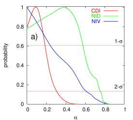
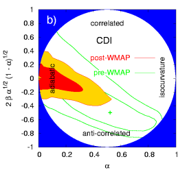
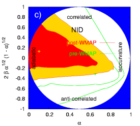
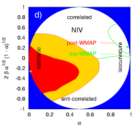
Figure 1: a) the likelihood function of the isocurvature fraction $\alpha$, for three different types of uncorrelated isocurvature modes (i.e., with the prior $\beta=0$); b) the 1 and 2-$\sigma$ contours of $\alpha$ and the cross-correlated mode coefficient $2\beta\sqrt{\alpha(1-\alpha)}$, for the CDM isocurvature mode: the small (red) contours are based on all the data, with one flat prior $n_{\rm iso}>0.6$, while the large (green) ones show the situation before WMAP, with an additional prior $\omega_{B}<0.037$; c) same as b) for NID; d) same as b) for NIV. The marginalization is approximated by a maximum likelihood fit of the other parameters for each pair of values $(\alpha,\beta)$.

In order to compute the $C_{l}$ coefficients of the temperature and polarization power spectra, as well as the matter spectra $P(k)$, we have used a CMB code developed by one of us (A.R.) which coincides, within 2% errors, with the values provided by CMBFAST for AD and CDI modes, and also includes the neutrino isocurvature modes as well as the cross-correlated power spectra. Note that the code defines the tilt of each power spectrum with respect to a pivot scale $k_{0}$ corresponding the present value of the Hubble radius, while CMBFAST uses $k_{0}=0.05$ Mpc^-1: so, the comparison of our results with those of Refs. WMAP for the CDI mixed model is not straightforward.

Table 1: The one-dimensional 2-$\sigma$ ranges on the isocurvature mode coefficients for the various models, uncorrelated (middle column) and correlated (right column).

model	$\alpha$	$\alpha$	$2\beta\,[\alpha(1-\alpha)]^{1/2}$
CDI	$<0.31$	$<0.47$	$-0.31$  to  $0.31$
BI	$<0.91$	$<0.95$	$-0.80$  to  $1.00$
NID	$<0.76$	$<0.77$	$-0.30$  to  $0.78$
NIV	$<0.60$	$<0.60$	$-0.77$  to  $0.35$

Results. We now describe the different bounds, summarized in Table I. For each specific mode, the probability distribution for $\alpha$ (uncorrelated case) and the likelihood contours in the $(\alpha,\,\beta)$ plane (correlated case) are shown on Fig. 1. The best-fitting parameter set for each model is given in Table II.

CDM isocurvature. Assuming no correlation between the adiabatic and CDI modes, we find an upper bound $\alpha<0.31$ at 95% c.l.. The deviation from a pure adiabatic model does not improve the goodness-of-fit, since the minimum $\chi^{2}$ value goes from 1478.8 to 1478.3, while the number of degrees of freedom decreases from 1435 to 1433. The situation does not change significantly when we include a possible correlation: the minimum $\chi^{2}$ is still around 1478.0, and the individual 2-$\sigma$ bounds on the coefficients read $\alpha<0.47$ and $-0.31<2\beta\sqrt{\alpha(1-\alpha)}<0.31$ at 95% c.l.. Most of the constraints on this model come from the WMAP TT power spectrum. For comparison, we repeated our analysis replacing WMAP and ACBAR by the Wang et al. Wang:2002rt CMB data compilation, which includes all the pre-WMAP temperature data. In that case, the results exhibit a wide parameter degeneracy (as indicated by previous studies Trotta:2001yw ; Amendola:2001ni ), and a large fraction of anti-correlated isocurvature modes cannot be excluded, up to $(\alpha,\,\beta)=(0.9,-1)$, provided one allows for a very large baryon fraction. Therefore, we conclude that the WMAP TT data is very powerful in constraining the isocurvature fraction. On the other hand, we checked explicitly that the effect of the WMAP TE power spectrum is not very strong with respect to that of TT.

In the curvaton scenario, the case in which the CDM is created before the curvaton decay while the curvature perturbations are small, corresponding to $(\alpha,\,\beta)=(0.9,\,-1)$ in our notation (3), is completely excluded, as already emphasized in Ref. Gordon:2002gv . The case in which the CDM is created by the decay of the curvaton leads to $\beta=1$; with such a prior, we obtain a sharp 2-$\sigma$ bound: $\alpha<0.04$ or, in the notation of Ref. Amendola:2001ni , $B<0.2$ (the authors of Ref. Gordon:2002gv obtain a more restrictive bound $B<0.43\ \Omega_{\rm B}/\Omega_{\rm M}\sim 0.1$, presumably because they use the curvaton–motivated assumption $n_{\rm iso}=n_{\rm ad}$). We can rewrite this bound as a constrain on the fraction $r=\Omega_{\sigma,\,{\rm decay}}$ since, in these models, $B=3(1-r)/r$. In our case, $B<0.2$ implies $1-r<0.0625$.

Table 2: The best fit values of the parameters for the adiabatic (AD), uncorrelated (CDI, etc.), and correlated (c-CDI, etc.) isocurvature models, with the corresponding $\chi^{2}$ and number of degrees of freedom $\nu$. For the NIV uncorrelated model, the best-fit occurs for $\alpha=0$ (i.e., purely adiabatic).

model	$\omega_{\rm B}$	$\omega_{\rm cdm}$	$\Omega_{\Lambda}$	$n_{\rm ad}$	$n_{\rm iso}$	$\alpha$	$\beta$	$\chi^{2}/\nu$
AD	$0.021$	$0.12$	$0.70$	$0.95$	$-$	$-$	$-$	$1478.8/1435$
CDI	$0.023$	$0.12$	$0.73$	$0.99$	$1.02$	$0.10$	$-$	$1478.3/1433$
BI	$0.023$	$0.12$	$0.73$	$0.99$	$1.02$	$0.72$	$-$	$1478.3/1433$
NID	$0.023$	$0.12$	$0.73$	$0.99$	$0.95$	$0.37$	$-$	$1478.2/1433$
NIV	$0.021$	$0.12$	$0.70$	$0.95$	$-$	$0$	$-$	$1478.8/1433$
c-CDI	$0.022$	$0.12$	$0.71$	$0.97$	$1.23$	$0.001$	$1$	$1478.0/1432$
c-BI	$0.022$	$0.12$	$0.71$	$0.97$	$1.23$	$0.03$	$1$	$1478.0/1432$
c-NID	$0.022$	$0.12$	$0.73$	$0.97$	$1.04$	$0.10$	$0.26$	$1477.7/1432$
c-NIV	$0.021$	$0.12$	$0.71$	$0.95$	$0.71$	$0.03$	$-1$	$1477.5/1432$

Baryon isocurvature. The case of baryon isocurvature modes is qualitatively similar to that of CDI modes, since the spectra are simply rescaled by a factor $\Omega_{\rm B}^{2}/\Omega_{\rm cdm}^{2}$ ($\Omega_{\rm B}/\Omega_{\rm cdm}$) for the isocurvature power (cross-correlation) components: thus, significantly larger values of $\alpha$ will be allowed in the baryon case. Some approximate results for the BI modes could be deduced from the CDI results by an overall rescaling of the $\alpha$ parameter. However, we performed an exact analysis, and found the following bounds: $\alpha<0.91$ (uncorrelated case), or $\alpha<0.95$ and $-0.8<2\beta\sqrt{\alpha(1-\alpha)}<1$ (correlated case). In each case, the minimum $\chi^{2}$ is, by definition, the same as for the CDI case. We provide the best-fit parameters in Table I, but for brevity we do not show this case in the figures.

In the curvaton scenario, the case in which the baryon number is created before the curvaton decay while the curvature perturbations are small, corresponding to $(\alpha,\,\beta)=(0.9,\,-1)$, is also excluded at several $\sigma$’s, as previously found by in Ref. Gordon:2002gv . The case in which the baryon number is created by the decay of the curvaton predicts $\beta=1$; we then find $\alpha<0.5$, or $B<1$.

Neutrino density isocurvature. The 2-$\sigma$ bound for the uncorrelated case is $\alpha<0.76$, while for the correlated adiabatic and neutrino mode we obtain $\alpha<0.77$ and $-0.30<2\beta\sqrt{\alpha(1-\alpha)}<0.78$. The best-fitting models for the two cases are still extremely close to the adiabatic model, leading to no significant improvement in the likelihood, $\Delta\chi^{2}=0.6$ vs. $\Delta\chi^{2}=1.1$, respectively. Note that with the pre-WMAP CMB data plus the 2dFGRS power spectrum, significantly larger fractions, up to $(\alpha,\,\beta)=(0.9,\,-0.6)$, of correlated NID modes were then allowed, but are now excluded with great confidence.

The authors of Ref. Lyth:2002my discuss an interesting mechanism under which the curvaton could generate some fully correlated or anticorrelated NID modes, through inhomogeneities in the neutrino/antineutrino asymmetry parameter. However, our bounds for these cases are very restrictive, $\alpha<0.18$ (correlated), or $\alpha<0.02$ (anticorrelated). In the notation of Ref. Amendola:2001ni , this is equivalent to $B<0.47$ or $B<0.14$, respectively.

Neutrino velocity isocurvature. Again, the presence of such a mode is not significantly favored: in the uncorrelated case, the best-fitting model is still the pure adiabatic one ($\alpha=0$), while in the correlated case the $\chi^{2}$ improvement is only $\Delta\chi^{2}=1.3$. The impact of WMAP on these bounds is spectacular. Using only the pre-WMAP CMB data compilation and the 2dFGRS power spectrum, we find that half of the parameter space (with $0<\alpha<1$ and $0<\beta<1$) was allowed until recently (at the expense of an unnaturally high baryon fraction and scalar tilt).

Conclusions. Using the recent measurements of temperature and polarization anisotropies in the CMB by WMAP, as well as the matter power spectrum measured by 2dFGRS, we obtained very stringent bounds on a possible isocurvature component in the primordial spectrum of density and velocity fluctuations. We have considered both correlated and uncorrelated adiabatic and isocurvature modes, and put strong constraints on the curvaton scenario of primordial perturbations.

References

- (1) A. D. Linde, Phys. Lett. B 158, 375 (1985); L. A. Kofman and A. D. Linde, Nucl. Phys. B 282, 555 (1987); S. Mollerach, Phys. Lett. B 242, 158 (1990); A. D. Linde and V. Mukhanov, Phys. Rev. D 56, 535 (1997); M. Kawasaki, N. Sugiyama and T. Yanagida, Phys. Rev. D 54, 2442 (1996); P. J. E. Peebles, Astrophys. J. 510, 523 (1999).
- (2) D. Polarski and A. A. Starobinsky, Phys. Rev. D 50, 6123 (1994); M. Sasaki and E. D. Stewart, Prog. Theor. Phys. 95, 71 (1996); J. García-Bellido and D. Wands, Phys. Rev. D 53, 5437 (1996); M. Sasaki and T. Tanaka, Prog. Theor. Phys. 99, 763 (1998).
- (3) C. Gordon, D. Wands, B. A. Bassett and R. Maartens, Phys. Rev. D 63, 023506 (2001); N. Bartolo, S. Matarrese and A. Riotto, Phys. Rev. D 64, 123504 (2001); D. Wands, N. Bartolo, S. Matarrese and A. Riotto, Phys. Rev. D 66, 043520 (2002); F. Di Marco, F. Finelli and R. Brandenberger, Phys. Rev. D 67, 063512 (2003).
- (4) D. Langlois, Phys. Rev. D 59, 123512 (1999); D. Langlois and A. Riazuelo, Phys. Rev. D 62, 043504 (2000); S. Tsujikawa, D. Parkinson and B. A. Bassett, Phys. Rev. D 67, 083516 (2003).
- (5) G. Efstathiou and J. R. Bond, Mon. Not. R. Astron. Soc. A 218, 103 (1986); 227, 33 (1987); P. J. E. Peebles, Nature 327, 210 (1987). H. Kodama and M. Sasaki, Int. J. Mod. Phys. A 1, 265 (1986); 2, 491 (1987); S. Mollerach, Phys. Rev. D 42, 313 (1990).
- (6) A. K. Rebhan and D. J. Schwarz, Phys. Rev. D 50, 2541 (1994); M. Bucher, K. Moodley and N. Turok, Phys. Rev. D 62, 083508 (2000); Phys. Rev. Lett. 87, 191301 (2001).
- (7) D. H. Lyth and D. Wands, Phys. Lett. B 524, 5 (2002); T. Moroi and T. Takahashi, Phys. Lett. B 522, 215 (2001); T. Moroi and T. Takahashi, Phys. Rev. D 66, 063501 (2002).
- (8) D. H. Lyth, C. Ungarelli and D. Wands, Phys. Rev. D 67, 023503 (2003).
- (9) C. L. Bennett et al. [The WMAP Collaboration], astro-ph/0302207; L. Page et al., astro-ph/0302220; H. V. Peiris et al., astro-ph/0302225.
- (10) C. L. Kuo et al. [The ACBAR Collaboration], astro-ph/0212289; J. H. Goldstein et al., astro-ph/0212517.
- (11) J. A. Peacock et al. [The 2dFGRS Collaboration], Nature 410, 169 (2001); W. J. Percival et al., Mon. Not. R. Astron. Soc. A 327, 1297 (2001); 337, 1068 (2002).
- (12) R. Stompor, A. J. Banday and K. M. Gorski, Astrophys. J. 463, 8 (1996); P. J. E. Peebles, Astrophys. J. 510, 531 (1999); E. Pierpaoli, J. García-Bellido and S. Borgani, JHEP 9910, 015 (1999); M. Kawasaki and F. Takahashi, Phys. Lett. B 516, 388 (2001); K. Enqvist, H. Kurki-Suonio and J. Väliviita, Phys. Rev. D 62, 103003 (2000); 65, 043002 (2002).
- (13) R. Trotta, A. Riazuelo and R. Durrer, Phys. Rev. Lett. 87, 231301 (2001); Phys. Rev. D 67, 063520 (2003).
- (14) L. Amendola, C. Gordon, D. Wands and M. Sasaki, Phys. Rev. Lett. 88, 211302 (2002).
- (15) C. Gordon and A. Lewis, astro-ph/0212248.
- (16) J. Väliviita and V. Muhonen, astro-ph/0304175.
- (17) from http://www.hep.upenn.edu/~max/cmblsslens.html; a previous version is described in X. Wang, M. Tegmark, B. Jain and M. Zaldarriaga, astro-ph/0212417.