The VIRMOS deep imaging survey II:
CFH12K BVRI optical data for the 0226-04 deep field

In this paper we describe in detail the reduction, preparation and reliability of the photometric catalogues which comprise the CFH12K-VIRMOS deep field. This region, consisting of four contiguous pointings of the CFH12K wide-field mosaic camera, covers a total area of $1.2\deg^{2}$. The survey reaches a limiting magnitude of $B_{AB}\sim 26.5$, $V_{AB}\sim 26.2$, $R_{AB}\sim 25.9$ and $I_{AB}\sim 25.0$ (corresponding to the point at which our recovery rate for simulated point-like sources sources falls below $50\%$). In total the survey contains 90,729 extended sources in the magnitude range $18.0<I_{AB}<24.0$. We demonstrate our catalogues are free from systematic biases and are complete and reliable down these limits. By comparing our galaxy number counts to previous wide-field CCD surveys, we estimate that the upper limit on bin-to-bin systematic photometric errors for the $I-$ limited sample is $\sim 10\%$ in this magnitude range. We estimate that $68\%$ of the catalogues sources have absolute per co-ordinate astrometric uncertainties less than $|\Delta\alpha|\sim 0.38\arcsec$ and $|\Delta\delta|\sim 0.32\arcsec$. Our internal (filter-to-filter) per co-ordinate astrometric uncertainties are $|\Delta\alpha|\sim 0.08\arcsec$ and $|\Delta\delta|\sim 0.08\arcsec$. We quantify the completeness of our survey in the joint space defined by object total magnitude and peak surface brightness. We also demonstrate that no significant positional incompleteness effects are present in our catalogues to $I_{AB}<24.0$. Finally, we present numerous comparisons between our catalogues and published literature data: galaxy and star counts, galaxy and stellar colours, and the clustering of both point-like and extended populations. In all cases our measurements are in excellent agreement with literature data to $I_{AB}<24.0$. This combination of depth and areal coverage makes this multi-colour catalogue a solid foundation to select galaxies for follow-up spectroscopy with VIMOS on the ESO-VLT and a unique database to study the formation and evolution of the faint galaxy population to $z\sim 1$ and beyond.

1 Introduction

Deep multi-colour observations remain one of the simplest and most useful tools at our disposal to investigate the evolution and properties of the faint galaxy population. The first digital studies of the distant Universe (Metcalfe et al., 1991; Lilly et al., 1991; Tyson & Seitzer, 1988) pushed catalogue limiting magnitudes beyond the traditional $B_{J}=24$ boundary of previous photographic works. They provided the first glimpse of the Universe at intermediate redshifts and tentative upper limits on the numbers of $z>3$ galaxies (Guhathakurta et al., 1990). Following these studies, thousand-object spectroscopic surveys in the mid-nineties (Ellis et al., 1996; Lilly et al., 1995a), combined with reliable photometry provided by charge-coupled devices (CCDs) mounted on 4m telescopes, sketched out for the first time the broad outlines of galaxy and structure evolution for normal $L^{*}$ galaxies in the redshift range $0<z<1$ (Le Fèvre et al., 1996; Lilly et al., 1995b).

At higher redshifts, the Hubble Deep Fields project (Williams et al., 1996) has demonstrated just how much can be accomplished beyond the spectroscopic limit of even 10m telescopes, provided photometric observations are sufficiently accurate. And in the last five years, searching for the passage of the Lyman break through broad-band filters has proved to be an extremely efficient way to locate objects at $z>3$ and above (Steidel et al., 1996; Madau et al., 1996; Steidel & Hamilton, 1993). These recent studies have provided a unique insight into the formation of large-scale structures and the relationship between mass and light in the regime where theoretical predictions depend sensitively on the underlying model assumptions (Adelberger et al., 1998). Meanwhile, at lower redshifts, the 2dF, 2MASS and Sloan surveys (Colless et al., 2001; Jarrett et al., 2000; York et al., 2000) are now providing us with a detailed picture of local Universe and a solid reference point for studies of the distant Universe.

To progress beyond these works at $z\sim 1$ demands imaging catalogues at least an order of magnitude larger than previously available from surveys based on single CCD detectors. One simple reason is that many objects of interest are rare; surface densities of Lyman-break galaxies, for instance, are around $\sim 1\leavevmode\nobreak\$arcmin^-2 at $I_{AB}<24.0$; amassing large samples of such galaxies requires coverage of a correspondingly large area of sky. In the recent years, large format multiple-CCD cameras such as the University of Hawaii’s 8K camera (UH8K; Luppino et al. (1994)), containing many separate CCD detectors and with a field of view of around $\sim 0.25$ deg² have become available and several surveys are now underway or have been recently completed using these cameras. For example, the Canada-France Deep Fields Survey (CFDF) covered three survey fields of the Canada-France Redshift Survey (CFRS; Lilly et al., 1995a) with the UH8K camera, providing $UBVI$ photometry for around $50,000$ objects (McCracken et al., 2001). With even larger, more efficient instruments such as the Canada-France-Hawaii Telescope’s 12K mosaic camera (CFH12K) it has now become feasible to conduct surveys subtending degree scales on the sky and reaching mean redshifts of $z\sim 1$. Furthermore, the advent of very high throughput spectrographs such as VIMOS (Le Fèvre et al., 2000) demands a new generation of wide-area deep digital survey catalogues in which systematic errors are rigorously controlled. It is also important to develop robust and reliable tools which can effectively deal with the even larger volumes of data which will be produced by the forthcoming 500-night Canada-France-Hawaii-Telescope Legacy Survey (CFHTLS) project which will use the new $1\deg^{2}$ field-of-view MEGACAM instrument (Boulade et al., 2000).

In this paper we describe $BVRI$ photometric observations which have been carried out in the VIRMOS-VLT deep field, a $1.2\leavevmode\nobreak\ \deg^{2}$ high galactic latitude field of low galactic extinction which will be the centrepiece of the VIRMOS-VLT deep spectroscopic survey (VVDS; Le Fèvre et al., 2001). Several tens of thousands of galaxy spectra will be acquired here to a limiting magnitude of $I_{AB}<24.0$. Observations described in this paper were made using the CFH12K mosaic camera: the broad spectral response and sensitivity of 12K, compared to previous-generation cameras such as the UH8K, make it an ideal instrument for this kind of survey (the DEEP2 redshift survey (Davis & Faber, 1998) are also using the CFH12K camera for survey pre-selection). In addition to the core $BVRI$ dataset described here, near-ultraviolet, near-infrared, X-ray and 1.4 GHz radio observations have also been carried out in this field, and will be presented in forthcoming papers. A companion paper (Le Févre et al., paper I) describes the overall strategy of the survey. Finally, a third paper will describe shallower optical data. This comprises three $4\leavevmode\nobreak\ \deg^{2}$ fields (the fields at 14hrs, 22hrs and 10hrs) and a $2\leavevmode\nobreak\ \deg^{2}$ extension to the field described here. In each of these fields spectra will be acquired from a sample of galaxies magnitude limited at $I_{AB}=22.5$.

This paper is organised as follows. In Section 2 we describe observations which were carried out; Section 3 describes how this data was reduced and includes details of how both astrometric and photometric solutions were computed to produce the final output images. In Section 3.5 we explain how object catalogues were produced from these images. In Section 4 we present a detailed quality assessment of the catalogues, where comparisons are made to existing deep catalogues. Our conclusions and summary are presented in Section 5.

2 Observations

This paper describes the F02 deep field of the VIRMOS-VLT survey. This field is centred at $02^{h}26^{m}00^{s}$ $-04^{\circ}30^{\prime}00^{\prime\prime}$ (J2000) which corresponds to a galactic latitude and longitude of $(172.0,-58.0)$ respectively. All observations described here were carried out using the CFH12K camera over a series of three observing runs from November 1999 to October 2000. The CFH12K is a 12,288 by 8192 pixel mosaic camera comprising twelve $2048\times 4096$ 15 micron pixel thinned backside illuminated MIT Lincoln Laboratories CCID20 devices. It has a total field of view of $42\arcmin\times 28\arcmin$ (Cuillandre et al., 2000). The average gain over all CCDs is $1.6e^{-}$/ADU. The pixel scale of the detector is approximately $0.205\arcsec/$pixel. The CFHT wide-field corrector produces a radial distortion amounting to $\sim 15$ pixels at the camera field of view (Cuillandre et al., 1996) which necessitates resampling our images before stacking. In total, the F02 deep field comprises four pointings of CFH12K in four filters covering a total area of $1.2\deg^{2}$.

Cosmetic quality of the detectors is generally good, with less than 200 bad columns in total, most of which are concentrated on a single detector. In addition, CFHT provides pixel masks which allow these bad pixels to be easily removed. The average gap between the charge coupled devices (CCDs) in the east west-direction is $7.8^{\prime\prime}$, whereas the north-south gap is $6.8^{\prime\prime}$. To fill these gaps in the final stacked mosaic, exposures were arranged in a dither pattern of radius $15^{\prime\prime}$. Figure 1 shows the layout of all $I-$band observations made on the field. Each rectangular box corresponds to the outline of one CCD image. At the scale of this plot it is not possible to see the dither pattern displacements.

Exposure times per image in each filter were typically 1800s for $B$, $1080s$ for $V$, $1200s$ for $R$ and $720s$ for $I$. The total exposure times in each of the four filters at each of the four pointings are listed in Table 1. In Figure 2 we show the distribution of full-width half-maximum (FWHM) seeing values for all the input images. All data with FWHM values greater than $1.2^{\prime\prime}$ were discarded.

Field	R.A. (2000)	Dec. (2000)	Band	Exposure time	Median seeing	Completeness limit
				(P1,P2,P3,P4)(hours)	(arcsec)	($AB$ mags)
0226-0430	02:26:00	$-$04:30:00	B	6.0, 5.5, 5.5, 5.0	0.9	26.5
			V	4.0, 7.0, 7.0, 4.0	0.8	26.2
			R	3.8, 3.1, 3.7, 3.3	0.8	25.9
			I	3.8, 3.2, 3.0, 2.8	0.8	25.0

Table 1: Details of the images used. We list the total integration time in each of the four pointings and the completeness limit of each filter, based on simulations described fully in Section 4.1.

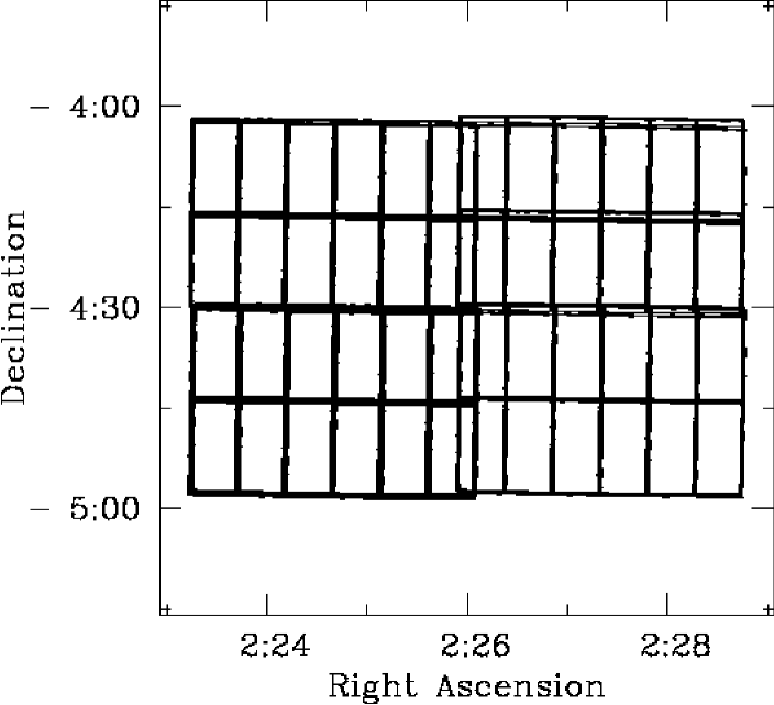
Figure 1: An outline of all CCD frames contained in the $I-$ band stack. Shown in this Figure are four separate pointings of the CFH12K camera. At each pointing there are 7-8 individual exposures comprising 12 CCDs in each. At the scale of this plot, it is not possible to see the displacement caused by the dither pattern offsets.

Figure 2: Seeing distribution for CCD images used in the F02 mosaic for each of the four filters. The dashed line shows the median seeing; note that in all cases this is less than $1^{\prime\prime}$. All images with a seeing higher than $1.2^{\prime\prime}$ were discarded and are not shown in this Figure.

3 Data reductions

Reducing observations taken by mosaic camera detectors present unique challenges in terms of the quantity of data which must be processed. For the project described in this paper, several thousand separate CCD images were processed totalling several hundred gigabytes of data; at least double this quantity of disk space is needed to combine these images into a single mosaic. The very large volume of data involved meant that all processing was carried out at TERAPIX, a data reduction centre at the Institut d’Astrophysique de Paris designed specially to process large quantities of wide-field mosaic camera data. One of the principal objectives of the TERAPIX facility is to carry out high-level processing (image co-addition and catalogue extraction) for the CFHTLS survey. The software tools described here were developed in the context of this project, and are described in detail in the following Sections of this paper. These tools were designed to be as general as possible and will work on mosaic data from other telescopes and cameras. They are available at the TERAPIX web site.

Our data reduction technique involves first de-trending our raw data, then computing astrometric and photometric solutions for all input CCD frames. These solutions are then used to re-sample and stack all CCDs for each filter into a single contiguous mosaic, from which catalogues are then extracted. We now describe each of these steps in turn.

3.1 Prereductions

All data were pre-reduced using the Fits Large Image Processing Software (FLIPS) package. Pre-reductions followed the normal steps of overscan, bias and dark subtraction. Dark current for the CFH12K is negligible, around 3 $e^{-}$pix^-1 hr^-1. Following this, all images are then divided by a twilight flat. For data taken in $R$ and $I$ filters, fringe removal is accomplished by subtracting a $2\sigma$ clipped median super-flat. These superflats were typically constructed from around $60$ science images. At this stage all images are scaled so they have the same sky background. After pre-reductions, the gradient of the background variation is measured across the CCD frames. This is always less than $2\%$ and is typically $\sim 0.5\%$.

3.2 Computing the astrometric solution

Astrometry and relative photometry were computed using the “astrometrix” and “photometrix” tools, part of the “WIFIX” package for the reduction of wide–field images, developed in the context of the TERAPIX project. In the following sections we describe the algorithms underlying these tasks and how they were applied to our data. An important aspect of these procedures is that they are able to operate in an unattended mode; given the large volume of data involved, manual interactions must be kept to a minimum.

In the following discussion, the approximate area defined by one of our CFH12K frames is described as a ’pointing’; in the F02 field there are four pointings in total. To reach a specified depth in a given pointing, several images are required, and these exposures are offset from each other in a “dither sequence” which contains between five and ten exposures.

To co-add all these separate CCD images and produce a seamless output image requires a detailed knowledge of the astrometric solution of each CCD frame. However, computing an astrometric solution constrained only by an external astrometric catalogue will not produce a sufficiently accurate solution. This is because the intrinsic accuracy of even the best external catalogues have rms uncertainties of around $\sim 0.2\arcsec$ per co-ordinate. This level of accuracy (combined with low object sky densities) make astrometric solutions derived from these catalogues alone unsuitable for co-addition of frames. In our survey we wish to produce a single contiguous mosaic comprising four separate pointings in four separate bands. Overlapping images from different filters and adjacent pointings must be registered to sub-pixel accuracy (or an r.m.s. smaller than $\sim 0.1\arcsec$. For these reasons, we have developed a procedure in which the astrometric solution is constrained simultaneously by the external astrometric catalogue and an internal catalogue generated from matched objects in overlapping CCDs, both from objects in the same pointing and in adjacent pointings. Since our $I-$ band data generally have the best seeing, and the VIRMOS spectroscopic sample will be $I-$ selected , we compute an astrometric solution from the $I-$ band data first. We then use this stacked image to derive solutions for all other bands.

The astrometric catalogue we used is the United States Naval Observatory (USNO)-A2.0 (Monet, 1998) which provides the position of $\sim 0.5\times 10^{8}$ sources. After the removal of saturated and extended objects between 30 and 50 sources per CFH12K CCD frame are left (the distribution of astrometric sources is not homogeneous on the sky). Deutsch (1999), by carrying out comparisons with a sample of $\sim 300$ radio sources, estimate a radial positional accuracy of the USNO-A2.0 of $\sim 0.25^{\prime\prime}$ (defined as the radius enclosing $68\%$ of the objects).

We begin our astrometric procedure by extracting input catalogues from the ($I$-band data) using SExtractor Bertin & Arnouts (1996) on each input (flat-fielded and bias subtracted) image. Saturated sources were removed. A cross-correlation procedure was used to compute the initial offsets (generated by the dither sequence) between these catalogues and the astrometric reference catalogue.

The astrometric solution describes the transformation between pixel projection plane co-ordinates $(x,y)$ and spherical co-ordinates on the sky $\xi,\eta$, namely,

$$\xi=\sum^{p}_{i=0}\sum^{i}_{j=0}A_{ij}x^{i-j}y^{j}$$ (1)

$$\eta=\sum^{p}_{i=0}\sum^{i}_{j=0}B_{ij}x^{i-j}y^{j}.$$

This is equivalent to the TAN projection in Calabretta & Greisen (2002) but without the $\left(x^{2}+y^{2}\right)^{0.5}$ terms.

This solution is computed as follows: firstly, for each observing run we select an exposure for which the relative offsets between CCDs, rotation angles and scaling factors are computed. These values are then applied to all other exposures. In this way it is possible to use all the available data to compute the offset to the USNO. In order to further minimise the possibility of errors, we separate the exposures into groups where fields overlap by around 50% and then compute the offsets between exposures in the same group. The offset to the USNO must be the same for a given group and we take the median of these values.

Next, for each CCD we match image sources with the astrometric catalogue and recompute the linear part of the world coordinate system (WCS). We then compute a first-guess astrometric solution (Eq. 1 with $p=2$). At this stage, a database of overlapping sources from all CCDs and pointings (“master” catalogues) is also constructed.

In the final step we re-compute the astrometric solution for all CCDs, but this time including points both from the astrometric catalogues and from the overlapping sources catalogue. The equation is solved using as weights the positional uncertainties on each source: we assume $0.3\arcsec$ for the USNO sources, whereas for the overlapping sources we use the positional uncertainties given by SExtractor. The system of equations is solved by iteration. Three iterations with $p=3$ produces RMS per-coordinate uncertainties of $\sim 0.3\arcsec$ for the USNO sources and $\sim 0.05\arcsec$ for overlapping sources. Unfortunately, since the offsets between exposures in the same dithering sequence are small ($\leq 20-30\arcsec$), the astrometric solution is poorly constrained in some regions as overlapping sources are actually extracted from the same part of the CCD and are affected by the same distortion (discussed at length later in this section). We therefore decided to reduce the weighting of overlapping sources from exposures which come from the same dither sequence. For these objects, weights are divided by the number of frames in that dither.

Figure 3: Positions of USNO sources compared to point-like sources with $17.5<I_{AB}<22.0$ in the final $1.2$ deg² stacked image. The inner and outer circles (at $0.5\arcsec$ and $1.0\arcsec$) enclose 68% and 90% of all objects respectively. The dotted lines cross each other at the position of the centroid, which is at $(\Delta\alpha,\Delta\delta)=(-0.03\arcsec,0.00\arcsec)$.

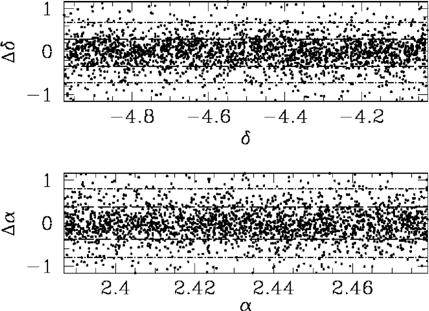
Figure 4: Positions of USNO sources compared to point-like objects in the $I$ stack as a function of right ascension and declination, displaying the uncertainty per co-ordinate. The inner dashed lines enclose $68\%$ of all sources and are at $|\Delta\alpha|\sim 0.38\arcsec$ and $|\Delta\delta|\sim 0.32\arcsec$; the outer dot-dashed lines enclosing $90\%$ of all sources are at $|\Delta\alpha|\sim 0.80\arcsec$ and $|\Delta\delta|\sim 0.70\arcsec$.

How do the positions of objects in the final $I-$ stack (produced after resampling and co-adding of all the input CCDs using this astrometric solution) compare to our input USNO-A2 catalogue? In Figure 3 we plot the difference between the positions of non-saturated, point-like sources in the $I-$ stack and their counterparts in the USNO-A2. The inner and outer circles enclose $68\%$ and $90\%$ of all the objects respectively, and have radii of $0.5\arcsec$ and $1.0\arcsec$. Figure 4 plots these residuals as a function of right ascension and declination. We note that our use of overlapping sources ensures that the accuracy of our internal astrometric solution is much higher, which is necessary if we are to successfully produce coadded images, as we will discuss now.

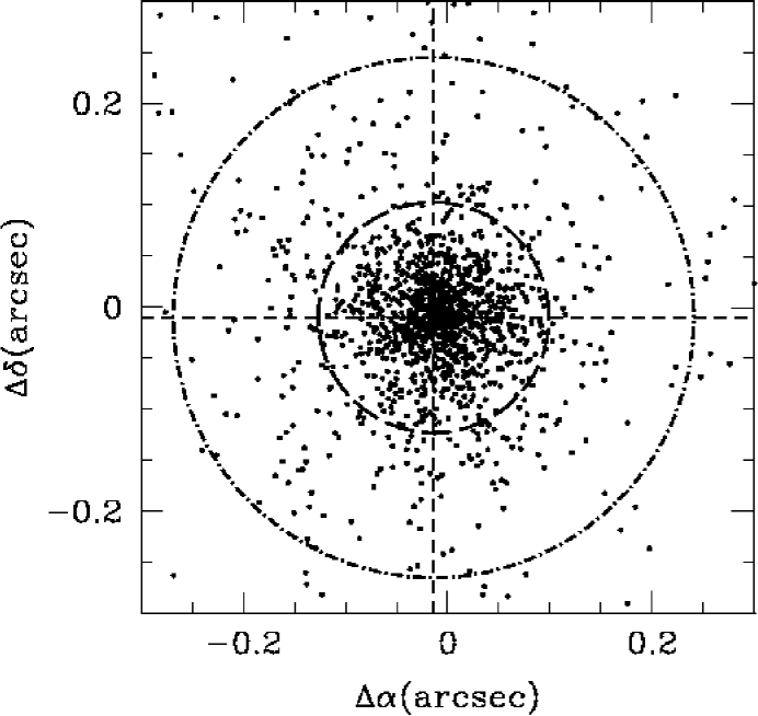
Figure 5: Positions of unsaturated point-like sources in the $I$ stack image compared with objects extracted from the $B$ stacked image. For clarity only one point in ten is shown. The circles at $0.11\arcsec$ and $0.26\arcsec$ enclose $68\%$ and $90\%$ of all sources respectively. The dotted lines cross each other at the position of the centroid, which is at $(\Delta\alpha,\Delta\delta)=(-0.01\arcsec,-0.01\arcsec)$.

To compute the astrometric solution for the $BVR$ data, we use as our reference catalogue a list of non-saturated point-like sources extracted from the $I-$ band stack. The procedure described above is then repeated using this catalogue. The surface density of these sources is much higher than that of the USNO-A2, and this approach allows images with different filters to be registered to a much higher accuracy. In Figure 5 we show the positional uncertainties between objects extracted in the $B$ and $I$ $1.2\leavevmode\nobreak\ \deg^{2}$ stacks. The inner circle and outer circles plotted at $0.11\arcsec$ and $0.26\arcsec$ enclose $68\%$ and $90\%$ of all objects. These figures indicate we have reached our required level of sub-pixel accuracy. In Figure 6 these positional uncertainties are plotted as a function of right ascension and declination.

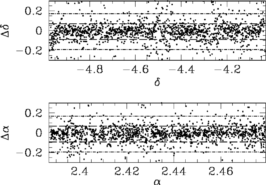
Figure 6: Residuals between $I$ and $B$ stacks as a function of right ascension and declination. The inner dashed lines enclose $68\%$ of all sources and are at $|\Delta\alpha|\sim 0.08\arcsec$ and $|\Delta\delta|\sim 0.08\arcsec$; the outer dot-dashed lines enclosing $90\%$ of all sources are at $|\Delta\alpha|\sim 0.18\arcsec$ and $|\Delta\delta|\sim 0.18\arcsec$.

Examining Figure 6, however, a potential problem becomes apparent. It is clear that there are regions in the stacked images where the rms astrometric uncertainty is much higher the average, although the area affected by these problems is small, less than $1\%$ of the total area. Two effects are responsible for these difficulties. The first is that the surface density of astrometric reference sources on the sky is not homogeneous: a situation can easily arise for example, in which there are few reference sources on one half of a CCD. Secondly, the dither offsets we use are too small to adequately sample the astrometric solution of the detector, and in many cases overlapping sources come from the same regions of the same CCDs. The net result is that in certain areas (mostly at the edges of CCD frames) the astrometric residuals are large. However, these regions are easily identified by comparing stacked images from each filter, and these areas are masked. The amount of area lost from these problems is small, less than a few percent of the total.

3.3 Photometric calibration

The photometric calibration is carried out in two steps. In the first, we determine an absolute calibration based on observations of standard star fields. In the second, we combine the absolute photometric calibration with a relative calibration computed using catalogues of overlapping sources to derive scaling factors which will be applied during stacking. We now describe both these steps in turn.

The absolute photometric calibration was performed by comparisons to a set of Landolt fields (Landolt, 1992). We were able to identify at least one set of photometric images from our observations, based on local sky conditions and stability of the object fluxes. Our observations are scaled to these photometric images using the procedure outlined below. Note that in this work, we do not attempt to calibrate each individual CCD frame independently, but instead calibrate the scaled, flat-fielded images (i.e., the entire mosaic). In other words, we assume that each CCD has the same colour equation. Since our observations were made, the CFH12K photometric performance has been extensively characterised as part of the CFHT queue observing program Elixir, which has determined zero-points and colour equations based on observations of several hundred standard star frames. The assumption that each CCD has the same photometric equation produces an overall photometric residual of less than $4\%$. These investigations also indicate that the CFH12K $BVR$ filters have negligible colour terms (less than 0.03 in $(B-V)$ and $(V-R)$ with respect to the Johnson Kron-Cousins system). Only in $I$ was a significant colour term found (quoting from the ELIXIR web pages):

$$I_{kc}=i_{cfh12k}+26.185-0.04(\kappa-1)+0.107(R-I),$$ (2)

where $\kappa$ represents the airmass, $R,I$ are Johnson magnitudes and $I_{kc}$ is the magnitude in Johnson Kron-Cousins system.

These zero-points and colour equations are broadly consistent with those determined from our survey data, but are of higher accuracy. Note that we do not actually use these colour equations in this work, and present all our magnitudes in the CFH12K instrumental system, defined by the combination of CFH12K detectors, filters and telescope. We do however convert our instrumental magnitudes to the “AB” magnitude system, (Oke, 1974) as follows: $B_{AB}=b_{cfh12k}-0.094$, $V_{AB}=v_{cfh12k}-0.007$, $R_{AB}=r_{cfh12k}+0.218$ and $I_{AB}=i_{cfh12k}+0.433$, computed from the CFH12K filter curves. Our zero-points are corrected for galactic extinction of $E(B-V)=0.027$ estimated at the centre of the field provided by the maps of Schlegel et al. (1998). As the galactic extinction is quite uniform over the field, we do not attempt to apply position-dependent magnitude corrections to our data.

After computing the absolute photometric calibration, and identifying photometric exposures in our data, we next compute the relative scaling exposure-to-exposure. The zero-point of each image $i$ may be written as the sum of two components:

$$Z_{i}=z^{\rm ph}+z^{\rm r}_{i},$$ (3)

where the photometric zero point $z^{\rm ph}$ is determined using standard stars and the relative zero point $z^{\rm r}_{i}$ incorporates the airmass correction and other changes in the atmospheric transparency. We assume that the relative zero point is the same for all the CCDs in a mosaic and that at least one image has been taken in photometric conditions, so that it may be used as reference. It is computed by minimising the average difference in magnitude of overlapping sources in different frames . Our approach is similar to that of Koranyi et al. (1998) except that we do not derive our coefficients by direct solution of a matrix inversion but by an iterative minimisation process.

The astrometric solution detailed in Section 3.2 provides a database of overlapping sources which can be used to compute the photometric offsets. We first extract from these catalogues pairs of objects from overlapping frames with magnitudes $m_{i},m_{j}$ and photometric uncertainties $w_{i},w_{j}$. For each pair we compute

$$\delta m_{ij}=\frac{\sum{w_{i}m_{i}}}{\sum{w_{i}}}-\frac{\sum{w_{j}m_{j}}}{\sum{w_{j}}}.$$ (4)

Our aim is to find the set of values $z_{i}$ which minimises

$$\delta m^{*}_{ij}=<m>_{i}+z_{i}-(<m>_{j}+z_{j})=\delta m_{ij}+(z_{i}-z_{j})$$ (5)

For each frame $i$ with overlapping sources in other $N_{\rm ov}$ frames, the zero point is:

$$Z_{i}=z^{\rm ph}+\frac{\sum_{j}^{N_{\rm ov}}{z_{j}-\delta m_{ij}}}{N_{\rm ov}}-\frac{\sum_{k}^{N_{\rm ph}}{z_{k}}}{N_{\rm ph}},$$ (6)

where we assume that $N_{\rm ph}$ frames are known to be photometric and that for them the average relative zero point is null. The effective airmass $\kappa$, of the coadded image is:

$$\kappa=\frac{\sum_{k}^{N_{\rm ph}}{\kappa_{k}}}{N_{\rm ph}}$$ (7)

Eq. 6 is iterated until $\frac{\sum_{i}^{N}{(\delta m^{*}_{ij})^{2}}}{N}$ converges or a maximum number of iterations (50) is reached.

3.4 Image resampling, stacking and flux scaling

Once the astrometric and photometric solutions have been computed for all the input CCDs, these images are combined to produce the final stack. This is carried out in a two-step process using a new image resampling tool, SWarp (Bertin et al., 2002).

In the first step, each input CCD is resampled and projected onto a subsection of the output frame (which covers all input images) using the astrometric solutions computed in Section 3.2. We use a tangent-plane projection, which is adequate given the relatively small size of our field. The flux scalings discussed in the previous Section are also applied at this stage. An interpolated, projected weight-map is also computed which incorporates information derived from bad pixel maps. Both for the weight-map and image data, interpolation is carried out using a “Lanczos-3” interpolation kernel. This kernel corresponds to a sinc function multiplied by a windowing function. It provides an optimal balance between preserving the input signal and noise structure and limiting ringing artifacts on image discontinuities (for instance, around bright stars and satellite trails). Additionally, at this stage a local sky background is computed at each pixel and subtracted, which ensures that the stacked image is free of large-scale background gradients.

In the final stage, all resampled images are coadded (with each pixel weighted by the appropriate weight map) to produce the final output image. Pixels are coadded using a median, which although sub-optimal for signal-to-noise properties, provides the best rejection of satellite trails and other cosmetic defects. In addition to the final coadded image, a total weight map is also produced containing information concerning how often each pixel has been observed. This weight-map is used during the detection and catalogue generation steps, outlined in the following sections. An important aspect of the resampling and stacking stage is that a single, large contiguous image is produced which contains all data, resulting in only one catalogue for each filter. No merging of catalogues is required. We set the size, pixel scale and orientation of the $BVR$ data to match the one computed for the $I$ data so that catalogues are easily extracted from these other images.

3.5 Catalogue preparation

To prepare merged $BVRI$ catalogues we locate objects using a separate detection image and then perform photometry in each bandpass at the positions defined by the detection image. This image is constructed using the $\chi^{2}$ technique outlined in Szalay et al. (1999), namely

$$y=\sum_{i=1}^{n}(a_{i}/\sigma_{i})^{2},$$ (8)

where $a_{i}$ represents the background-subtracted pixel value in filter $i$, $\sigma_{i}$ the rms noise at this pixel and $n$ is the number of filters (four in this case).

In the absence of sources, the distribution of sky values in this stacked image can be described as $\chi^{2}$ distribution with $n$ degrees of freedom. Detection and thresholding, therefore, have relatively simple interpretation in probabilistic terms. Our primary motivation in using this technique is to simplify the generation of multi-band catalogues and to reduce the numbers of spurious detections.

We produce this $\chi^{2}$ image from the four stacked images using SWarp which performs the local estimations of $\sigma_{i}$ and the sky background at each pixel (note that in version 1.21. of SWarp, used here, the output pixels in the generated $\chi^{2}$ images are actually $S=\sqrt{(y/n)}$). For the $\chi^{2}$ technique to work reliably, seeing variations across input images must be small (less than $\sim 20\%$) and moreover there must be the same number of input images at each pixel (a consequence of this is that detections may not be reliable in parts of the image where there is no coverage in all four bands). We have compared magnitudes of objects recovered with and without the use of the $\chi^{2}$ detection image and we find no evidence that it introduces any magnitude bias.

For objects to be included in our catalogues, they must contain at least three contiguous pixels with $S>2$ in the $\chi^{2}$ image. This corresponds to a per-pixel detection threshold of $2.8\sigma$. With this threshold we detect in total 460,447 sources. We chose this somewhat conservative threshold in order to minimise the numbers of false detections. However, as we shall see in the following sections, our catalogues are essentially complete at $I_{AB}=24$. This threshold is close to the ’optimal’ value where the probability of misclassifying object pixels as sky and sky pixels as objects is minimised (see Figure 1. of Szalay et al.).

In our catalogues, magnitudes are measured using Kron (1980)-like elliptical aperture magnitudes computed using SExtractor (the magauto parameter). These magnitudes provide the most reliable measurement of the object’s total flux (based on simulations carried out on our images), although they may be subject to blending effects if there are near neighbours. This is not a concern for us because our images in all bandpasses are far from the confusion limit and the numbers of objects affected are very small. We set a minimum Kron radius of $1.2^{\prime\prime}$, which means that for faint unresolved objects (where the Kron radius can be difficult to reliably determine), our “total” magnitudes will revert to simple aperture magnitudes. Colours are always measured at the same location (defined by the detection image) on each stack. Because there are many large, extended objects on our images, we also use magauto magnitudes to measure object colours. Once again, tests show that these colours revert to “aperture” colours for the majority of faint, unresolved objects in our catalogues. Measurements show that for total magnitudes in the range $18.0<I_{AB}<24.0$ the difference between the median galaxy colour using total and aperture magnitudes is less than 0.05 magnitudes.

We use the SExtractor flux_radius parameter to identify point-like sources, using object profiles measured in the $I-$band images with centroids derived from the $\chi^{2}$ image (of course, given that we have $BVRI$ photometry for all objects, a complementary approach would be to identify stellar sources based on best-fitting spectral templates; application of this technique to our data will be described in future papers). This parameter, denoted as $r_{1\over{2}}$, measures the radius which encloses a specified fraction of the object’s total flux (in this case, $50\%$). Fainter than saturation ($I_{AB}\sim 18$), point-like objects have a flux radius independent of magnitude. In our data, an added complication is that the seeing differs by around $20\%$ across the mosaic, which means this locus is slightly dispersed. To account for this, we used an “adaptive” classification technique. In this procedure, we divide the field into many sub-areas and compute the mode of $r_{1\over{2}}$ for objects within each box. Since point-like objects all have the same half-light radius this provides a robust measurement of the local seeing value. A search is then carried out for the bin which has a value of less than $20\%$ of the modal bin; all objects with $r_{1\over{2}}$ smaller than this are classified as stars.

Figure 7 demonstrates how this method works in practice. In the upper panel we show the half-light radii values as a function of $I_{AB}$ magnitude for all objects, normalised by the approximate mean value for the full field. In the lower panel, each object’s half-light radii has been divided by the local measurement. The heavy dots in both panels indicate the point-like objects located using the classifier. The separation between resolved and unresolved sources is considerably improved, and distinguishing between the two seems feasible until $I_{AB}\sim 22$, although in this work we adopt a conservative limit of $I_{AB}\sim 21.5$. Beyond this limit no classification is attempted.

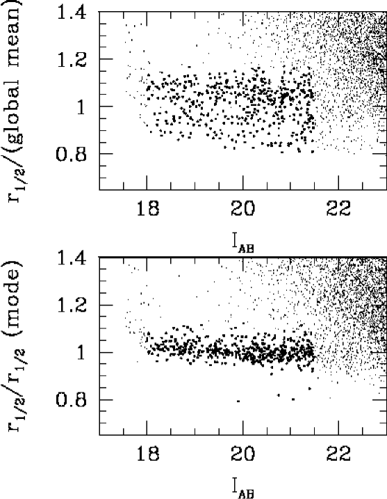
Figure 7: Object half-light radius as a function of $I_{AB}$ magnitude. In the upper panel, we show the half-light radius in pixels (normalised by full-field mean of 2.5 pixels) over the full mosaic both for point-like (solid points) and extended sources (light points). In the lower panel each object’s half-light radius has been normalised by the local mode, computed using the adaptive classifier (in both panels, for clarity, only a fraction of all objects are shown).

Finally, the catalogue was visually inspected by over-plotting on the images all non-saturated objects with $I_{AB}<24.0$. Areas contaminated by residual fringing, satellite trails and scattered light were flagged by drawing polygonal masks around them. All large bright stars and their corresponding diffraction spikes were also masked. In Figure 8 we show the distribution of galaxies with $18.0<I_{AB}<21.0$. Masked regions, outlined by polygons, are also indicated. In the magnitude range $18.0<I_{AB}<24.0$ we detect 90,951 extended objects not in the masked regions or at the borders of the image. In this area and magnitude range there are 2857 point-like sources. The total area of our survey, after masking is $1.18$ deg².

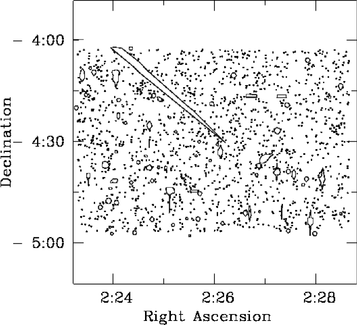
Figure 8: Distribution of bright galaxies. The points show galaxies (extended sources) with $18.0<I_{AB}<21.0$. Masked regions are also indicated.

4 Data quality assessment

In these sections we describe and present a series of quality assessment tests carried out on the $BVRI$ catalogues prepared in the previous sections.

4.1 Surface brightness selection effects and catalogue limiting magnitudes

Our objective here is to determine the photometric completeness of our survey in the plane defined by surface brightness and total magnitude. The importance of surface brightness selection effects in photometric surveys has already been discussed by several authors (Lilly et al., 1995a; Yoshii, 1993). In this work, an important objective of our simulations is to ensure that our data is fully complete and free from surface brightness selection effects at $I_{AB}=24.0$, the spectroscopic limit of the VLT-VIRMOS deep survey.

To estimate how surface brightness selection effects could affect our catalogues a variety of approaches may be used. For example, we might try to produce simulated objects with a variety of light profiles, such as exponential disks or $r^{1/4}$-law bulges. These objects could then be dimmed based on some physically motivated picture of how galaxies evolve and then coadded back into our image frames and their object parameters re-measured. In what follows, however, we adopt a purely empirical approach. We start by extracting $BVRI$ sub-areas of 100 bright, isolated galaxies from a $1024\times 1024$ subsection of the field. Our objective is to quantify, at each combination of magnitude and total surface brightness, how many objects are recovered by our selection procedure. Some of the surface-brightness/magnitude combinations are not physical, but we wished to introduce as few assumptions as possible about the evolution of the faint galaxy population into our simulations. A consequence of this approach, of course, is that interpreting the overall completeness requires additional information concerning where the faint galaxy population resides in the surface-brightness/magnitude plane.

To relocate our galaxies in the surface brightness/magnitude plane we reduce their total magnitude and surface brightnesses by dividing each object by some number to scale it to a fainter total magnitude. To reduce the surface brightness of the galaxies while keeping the same total magnitude, the galaxies were stretched using bilinear interpolation. After these alterations, the galaxies are added back into the subsections extracted from each of four bandpasses. Following this, objects are detected using the same procedures as in the real catalogues. We generate a $\chi^{2}$ detection sub-image and search for objects using our detection threshold (corresponding to three connected pixels having $S>2$). For each combination of $I_{AB}$ total magnitude and peak surface brightness (defined as the surface brightness of the brightest pixel in the recovered object) we measure the fraction of galaxies retrieved. To evaluate the numbers of spurious detections, all the images are multiplied by $-1$. As before, the $\chi^{2}$ image is generated and the flux measurement is carried out using SExtractor in dual image mode on the negative images. The number of initial detections will be the same since the chi-squared detection image generated from the negative images is the same as the chi-squared image generated from the positive images. However, since the measurement image is now negative, positive fluxes will be measured only for the false detections.

The results of these simulations are illustrated in Figure 9 where they are plotted in the plane defined by total magnitude and peak surface brightness. Filled dots show the position of all objects in the field; the solid line shows the location of the stellar locus. For each combination of total magnitude and peak surface brightness, the numbers indicate the percentage of objects which are recovered. The contour lines indicate the $50\%$, $70\%$ and $90\%$ completeness limits. The open circles show the spurious detections; we note that these spurious detections only become significant faintwards of $I_{AB}\sim 25$.

For point-like stellar objects at $I_{AB}=24.0$ our survey is essentially complete, with approximately $90\%$ of objects recovered at this combination of magnitude and surface brightness. At this magnitude our recovery fraction drops to $50\%$ for objects with peak surface brightnesses of around $\sim 25.5$ mag arcsec². Lilly et al. (1995a) have computed the tracks of typical galaxies in the surface-brightness magnitude plane, and their Figure 7 shows that most “normal” galaxies would be easily detected by our survey. Objects with extremely large half-light radii, such as the prototypical “Malin 1” low surface brightness galaxy could fall below our detection limits at higher redshifts. However, space-based observations suggests that the numbers of such extended, low-surface brightness objects at these magnitudes is actually quite low (Simard et al., 1999; Fasano et al., 1998). Most of the objects we detect in the real data (filled points in Figure 9) fall in quite a narrow locus in the surface-brightness/magnitude plane. Moreover, if we compare our total galaxy number counts at $I_{AB}=24.0$ with an average of measurements in North and South Hubble Deep Fields (Metcalfe et al., 2001) (presented in Section 4.3) we see that we are in good agreement at $I_{AB}=24$ with these much deeper counts. Based on these considerations, we conclude that our survey is essentially free of selection effects until at least $I_{AB}\sim 25$. Finally, we note that our simulations also show that at this limit our survey is free from spurious detections (represented as the open circles in Figure 9).

We have also carried out a set of simulations based on adding progressively fainter simulated stellar sources to a sub-section of the image stacks. The magnitudes at which we recover $50\%$ of the input sources is $26.5$,$26.2$,$25.9$ and $25.0$ for $BVRI$ filters respectively.

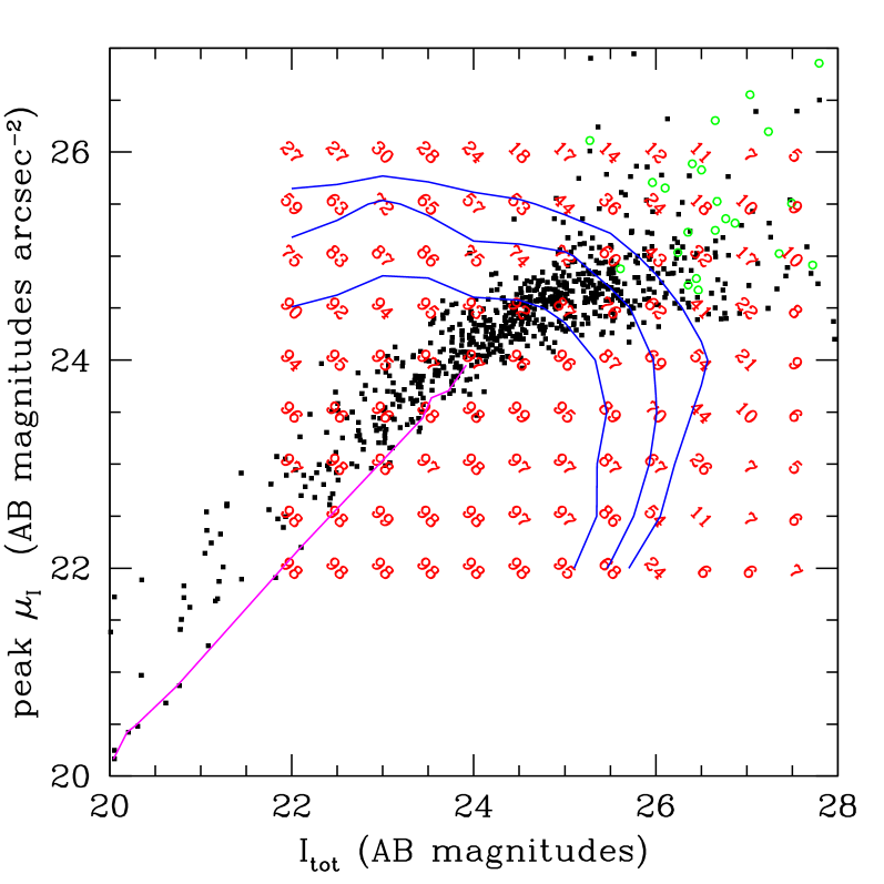
Figure 9: Peak surface brightness as a function of $I_{AB}$ total magnitude. Detected galaxies are shown as the black dots, the open circles show the spurious detections. The stellar locus is represented by the solid line. Most galaxies lie nearby to this locus. The contour lines indicate the $50\%$, $70\%$ and $90\%$ completeness limits. The numbers represent the fraction of objects recovered at each combination of total magnitude and peak surface brightness.

4.2 Catalogue completeness as a function of position

An important issue to address is how homogeneous the detection and measurement limits are over the entire mosaic, and how stable the images’ noise properties are as a function of location. To estimate this, we carried out a series of simulations aimed at measuring the incompleteness as a function of position for the full $I-$ band mosaic. In these simulations, we extracted $\sim 200$ sub-areas arranged in a grid over the mosaic. For each of these sub-areas, we added artificial stars at random positions using as a local seeing value the measurements derived in Section 3.5 (our intention in this experiment is not to provide a realistic assessment of the absolute value of the incompleteness but rather its positional variation, which is why we adopt the simplifying assumption of stellar profiles). Detection and measurement was then carried out using SExtractor, using detections weighted by the local detection weight-map. For several slices in magnitude, we measured what fraction of stars we recover at each position.

Our results are illustrated in Figure 10, where we plot the recovery fraction as a function of position for input objects in the magnitude range $23.75<I_{AB}<24.25$. Over most of the field, the recovery fraction is $>90\%$ (in good agreement with the result derived for point-like sources in the previous section). There are small regions where the completeness can be significantly lower; upon investigation, these areas appear to be populated by bright stars which were not excluded from the simulation. From these tests we conclude that there is no significant variation in completeness over the mosaic at $I_{AB}=24.0$.

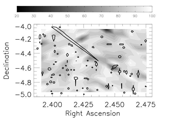
Figure 10: Measured incompleteness as a function of position (decimal declination and right ascension) for the $I$ band mosaic. The grey-scale contours indicate, at each position, the fraction of stellar objects which were recovered. Input magnitudes were distributed uniformly in the range $23.75<I_{AB}<24.25$. The thick lines show the location of the masked regions.

4.3 Galaxy and star counts

In this Section we compare the source counts of our catalogues of galaxies and stars (in reality, point-like and extended sources) to published compilations. The filled squares in Figure 14 shows $I_{AB}$-selected stellar number counts compared to the predictions of the model of Robin et al. (2002), computed at the galactic latitude of our survey. In the magnitude range $18<I_{AB}<21.5$ we measure the slope of the stellar number counts, $d\log N/dm$, as $\sim 0.14$. Our stellar counts and slope measurement are in in excellent agreement with model predictions (a detailed discussion of the properties of the stars in the survey will be presented in a future paper).

Differential galaxy number counts per square degree per half magnitude for $B$, $V$, $R$, and $I$ filters derived from our catalogue are represented as the filled circles in Figures 11, 12, 13 and 14. These counts are also listed in Table 2. We do not correct our counts for incompleteness, and show “raw” measurements. For our literature comparison, we include only measurements from recent digital surveys and omit earlier photographic works. We note how well the galaxy count measurements now agree well between the different surveys, in particular for the $B-$band measurements. It appears that the large scatter between different groups in previously presented compilations arose from uncertainties in photographic magnitude scales at the bright end and from the small fields of view of the previous generation of deep CCD surveys at the faint end. By contrast, in many large surveys today, systematic errors arising from absolute zero-point uncertainties dominate in almost every magnitude bin.

In general, our agreement with the literature measurements is excellent. In the $V-$ band, our counts are in good agreement with those of Cabanac et al. (2000), the CFDF measurements and those of Arnouts et al. (2001). The counts from Wilson (2003) appear to be systematically below all other measurements.

We have also carried out a more detailed bin-by-bin comparison with the $I_{AB}$ galaxy counts determined in the CFDF survey, which has comparable total area ($\sim 1$ $\deg^{2}$) to the present work. The CFDF counts differ at most from the present work by $\sim 10\%$ per bin. Given the large numbers of galaxies in each bin, this error is almost always larger than the combination of $\sqrt{N}$ Poisson counting errors and fluctuations induced by large scale structure (which is small for the fainter bins). Assuming this difference arises from uncertainties in the absolute zero-points of the CFDF and the present work, this would correspond to absolute zero-point uncertainty of $\sim 0.05$ magnitudes (estimated simply by calculating what zero-point shift minimises the difference in counts between the two surveys). This is in agreement with what we have estimated in Section 3.3 from observations of Landolt standard star fields.

We have also determined the slope $\alpha$ ($d\log N/dm$) of the galaxy counts, and these are reported in Table 3. Our $B$ and $I$ slopes agree well with reported CFDF survey values of $\sim 0.35$ and $\sim 0.47$ respectively. Fainter than $B_{AB}\sim 24$ we observe a slope flattening in the $B-$: for $24<B_{AB}<25.5$, we find $d\log N/dm\sim 0.3$, similar to that found by Metcalfe et al. (1995).

	$B$		$V$		$R$		$I$
AB Mag	$N_{gal}$	$\log N_{gal}$ $\deg^{-2}$	$N_{gal}$	$\log N_{gal}\deg^{-2}$	$N_{gal}$	$\log N_{gal}$ $\deg^{-2}$	$N_{gal}$	$\log N_{gal}\deg^{-2}$
18.0-18.5	37	1.50	137	2.06	303	2.41	332	2.45
18.5-19.0	78	1.82	251	2.33	346	2.47	462	2.59
19.0-19.5	119	2.00	335	2.45	508	2.63	811	2.84
19.5-20.0	176	2.17	550	2.67	793	2.83	1156	2.99
20.0-20.5	328	2.44	767	2.81	1157	2.99	1890	3.20
20.5-21.0	508	2.63	1182	3.00	1732	3.17	2796	3.37
21.0-21.5	882	2.87	1625	3.14	2476	3.32	4168	3.55
21.5-22.0	1247	3.02	2565	3.34	3930	3.52	6759	3.76
22.0-22.5	2312	3.29	4137	3.54	5922	3.70	9992	3.93
22.5-23.0	3813	3.51	6831	3.76	9241	3.89	13676	4.06
23.0-23.5	7014	3.77	11450	3.99	14006	4.07	19863	4.23
23.5-24.0	12771	4.03	19609	4.22	22235	4.28	28828	4.39
24.0-24.5	22130	4.27	30850	4.42	33632	4.45	39874	4.53
24.5-25.0	34448	4.47	43593	4.57	46362	4.59	47079	4.60
25.0-25.5	47255	4.60	54457	4.66	56686	4.68	43459	4.57

Table 2: Differential galaxy number counts. Counts are shown in half-magnitude bins selected in $(BVRI)_{AB}$. Also shown are the logarithmic counts, normalised to the effective area of the survey field ($1.18$ deg²).

Filter	Magnitude range	$d\log N/dm$
B	20.0-24.0	$0.45\pm 0.01$
B	24.0-25.5	$0.32\pm 0.04$
V	20.0-24.0	$0.40\pm 0.03$
R	20.0-24.0	$0.37\pm 0.03$
I	20.0-24.0	$0.34\pm 0.02$

Table 3: Best-fitting galaxy count slopes in $BVRI$ bands for our catalogue, computed in the specified magnitude ranges.

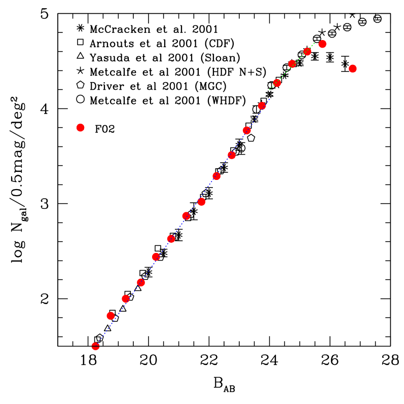
Figure 11: $B_{AB}$-selected galaxy counts (filled symbols), compared to a selection of recent results from the literature. The dotted lines shows the best fitting slope computed in the magnitude ranges $20.0<B_{AB}<24.0$ and $24.0<B_{AB}<25.5$. Error bars are smaller than our symbols and are not shown.

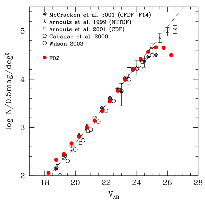
Figure 12: $V_{AB}$-selected galaxy counts (filled symbols), compared to a selection of recent results from the literature. Error bars are smaller than our symbols and are not shown.

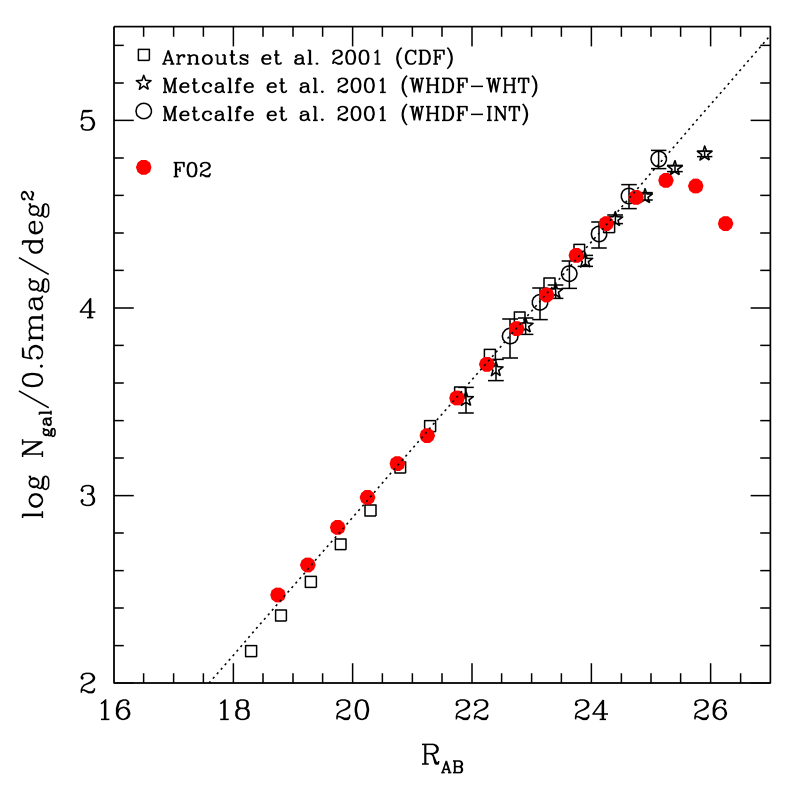
Figure 13: $R_{AB}$-selected galaxy counts (filled symbols), compared to a selection of recent results from the literature. Error bars are smaller than our symbols and are not shown.

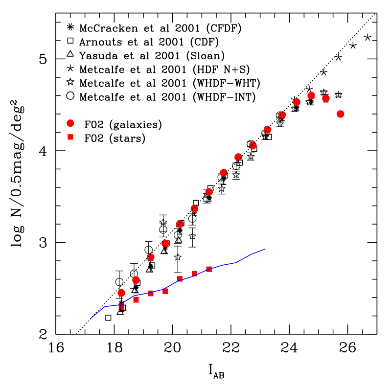
Figure 14: $I_{AB}-$ selected galaxy and star counts (filled circles and squares respectively), compared to a selection of recent results from the literature (open symbols). For the galaxy counts, in all cases our (Poisson) error bars are smaller than the symbols and are not plotted. The dotted line shows the best fitting slope computed in the magnitude range $20<I_{AB}<24$. The solid line shows the predictions of the galactic model of Robin et al., computed at the galactic latitude of our survey.

4.4 Stellar colours

In this Section we examine the relative and absolute photometric calibration by investigating the colours of stars distributed over our field.

The filled symbols in Figure 15 shows the $(B-V)_{AB}$ and $(V-I)_{AB}$ colours of point-like sources in our catalogue compared to synthetic colours generated by convolving the stellar spectral energy distributions of Pickles (1998) with the CFH12K filter set (open symbols). From this plot it is apparent that in $BVI$ filters our absolute calibration is accurate to within $\sim 0.05$ magnitudes.

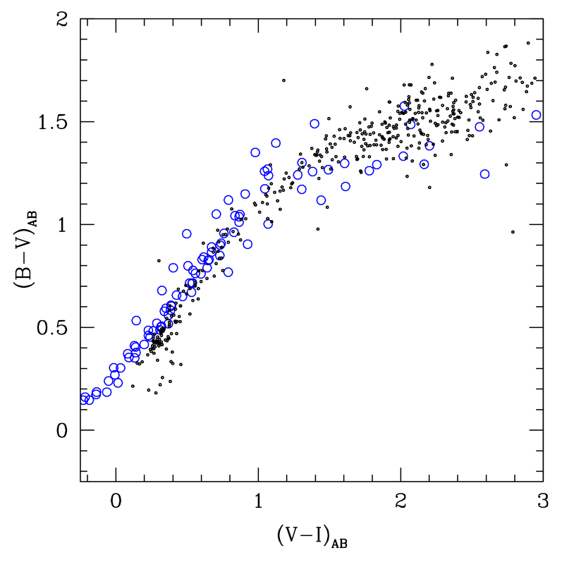
Figure 15: $(B-V)_{AB}$ vs $(V-I)_{AB}$ colours for (filled points) compared to synthetic colours computed from library of Pickles (open circles).

We also use measured colours of stars in our fields to investigate if there are systematic differences in stellar colours across the mosaic. The results of these tests are illustrated in Figures 16 where we plot the median $(B-V)_{AB}$, $(V-I)_{AB}$ and $(R-I)_{AB}$ colours of stars selected from each of the four pointings. It appears from these tests that over these four regions the relative differences in zero points is less than $0.05$ magnitudes for each of the four filters.

Figure 16: Stellar colours as a function of position for each of the four pointings. In each pointing we compute the median $(B-V)_{AB}$ and $(R-I)_{AB}$ colours in bins of $(V-I)_{AB}$ (upper and lower panels respectively). This is represented as the four different line styles. The regions are defined as follows: solid line: south-west, dotted line: north-east; dashed line: south-east, dot-dashed line: north-west.

4.5 Field galaxy colours

In this Section we compare our field galaxy colours (or, more accurately, extended sources) to those from other deep surveys. We compute the median $(B-V)_{AB}$ and $(V-I)_{AB}$ colours in half-magnitude bins as a function of $B_{AB}$ and $I_{AB}$ sample limiting magnitude. These measurements are shown as the solid lines in the upper and lower panels of Figure 17. The symbols show field galaxy colours measured from the CFDF survey. In both cases our agreement with the published values is excellent.

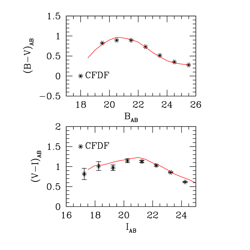
Figure 17: Field galaxy colours from our catalogues. In the upper panel, the solid line shows the median $(B-V)_{AB}$ galaxy colour computed in half-magnitude bins as a function of $B_{AB}$ limiting magnitude; in the lower panel, we show the median $(V-I)_{AB}$ colour as a function of $I_{AB}$ magnitude. In both cases we compare with colours from the CFDF survey (symbols).

We also investigate the distribution of galaxies in colour-colour space as a function of magnitude; this is illustrated in Figures 18, 19 and 20. In these Figures we compare our observed galaxy colours to model predictions for a range of progressively fainter magnitude slices. The grey-scales in these Figures are proportional to object number density, computed in 0.1 magnitude intervals in $(B-V)_{AB}$ and $(V-I)_{AB}$. Dotted lines show the path of late-type (E, S0) galaxies wheras early-type galaxies (Sa, Sc and Irregular) are represented by solid lines. Galaxy colours were computed at intervals of $0.1$ in redshift by applying the CFH12K filter response functions to model evolving spectral energy distributions generated using the “2000” revision of the GISSEL libraries (Bruzual & Charlot, 1993). Computations were made assuming a flat $\Lambda$-CDM cosmology. The e-folding times for the five tracks are $(0.3,1.0,2.0,4.0)$ Gyrs and “constant” for elliptical, S0, Sa, Sc and Irregular galaxy types respectively. Model galaxy zero-redshift colours (represented by the filled dots) are in good agreement with the colours reported in Mannucci et al. (2001). Finally, intergalactic absorption as modelled by Madau (1995) has also been added.

Figure 18 shows the bright magnitude slice at $18<I_{AB}<20$. In this Figure, most galaxies lie in a single well-defined region. From previous $I_{AB}$-selected galaxy redshift surveys such as the CFRS we know that at these magnitudes the median redshift of the faint galaxy population is around $z\sim 0.2$ (Crampton et al., 1995), and this is also roughly where the model tracks enter the locus occupied by the galaxy population. In addition, we note that the model tracks span very well all the observed colours in our survey.

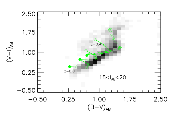
Figure 18: $(B-V)_{AB}$ vs $(V-I)_{AB}$ colour-colour diagram for galaxies with $18<I_{AB}<20$. The greyscale levels are proportional to the numbers of galaxies at each combination of $(V-I)_{AB}$ and $(B-V)_{AB}$ colour. The lines shows model tracks for five galaxy types (two early types, shown by the dotted lines, and three late-types, represented by the solid lines). Tracks are computed in the redshift range $0.0<z<0.4$ in intervals of $0.1$. Solid symbols show the location of the $z=0$ point for each track.

For the intermediate magnitude slice at $20<I_{AB}<22$, illustrated in Figure 19, the (predominantly late-type) galaxy population occupies two distinct locii, and in colour-colour space there is a comparatively well-defined separation between high ($z>0.4$) and low ($z<0.4$) redshift galaxies. For the very faintest magnitude slice, $22<I_{AB}<24$, the sharp distinction has been removed, and all parts of the colour-colour diagram are equally populated. In general, our extended source colours are in agreement with the existing model tracks.

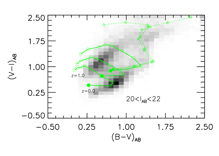
Figure 19: Colour-colour diagram for galaxies with $20<I_{AB}<22$. For this Figure, model tracks span the redshifts range $0.0<z<1.0$.

Figure 20: Colour-colour diagram for galaxies with $22<I_{AB}<24$. Model tracks are computed from $0.0<z<3.0$.

4.6 Clustering of point-like sources

In this Section and the following one we investigate the clustering properties of point-like and extended sources in our catalogues. To do this, we use the well-known projected two-point angular correlation function, $\omega(\theta)$, which measures the excess of pairs separated by an angle $\theta,\theta+\delta\theta$ with respect to a random distribution. This statistic is useful for our purposes because it is particularly sensitive to any residual variations of the magnitude zero-point across our stacked images.

We first measure the angular correlation function $\omega(\theta)$ of the stellar sources. As stars are unclustered, we expect that if our magnitude zero-points and detection thresholds are uniform over our field then $\omega(\theta)$ should be zero at all angular scales. For this test, we consider two magnitude limited samples: point-like sources with $18.0<I_{AB}<20.0$ and those with $20.0<I_{AB}<21.5$. We measure $\omega(\theta)$ using the standard Landy & Szalay (1993) estimator, i.e.,

$$\omega(\theta)={\mbox{DD}-2\mbox{DR}+\mbox{RR}\over\mbox{RR}}$$ (9)

with the $DD$, $DR$ and $RR$ terms referring to the number of data–data, data–random and random–random galaxy pairs between $\theta$ and $\theta+\delta\theta$. We use logarithmically spaced bins with $\Delta\log(\theta)=0.2$.

Our results are displayed in Figure 21. For both magnitude cuts, at scales $-2.5<\log(\theta)<0.0$ the measured correlation amplitudes are consistent with zero.

Figure 21: Angular clustering of stellar sources, $\omega(\theta)$ as a function of the logarithm of the angular separation in degrees. Filled squares represent objects with $18.0<I_{AB}<20$; open circles show sources with $20.0<I_{AB}<21.5$. For clarity, the fainter magnitude slice has been slightly offset in $\log(\theta)$ from the brighter one.

4.7 Clustering of extended sources

The angular clustering of field galaxies, parametrised by $\omega(\theta)$ provides important information concerning the galaxy distribution. Many studies have measured $\omega(\theta)$ for progressively larger samples of galaxies reaching to fainter and fainter magnitudes (see, for example, Brainerd et al. (1994); Roche et al. (1993); Efstathiou et al. (1991)). The advent of mosaic detector arrays means it is now possible to measure the angular clustering of field galaxies on degree scales at $z\sim 1$ with samples reaching magnitude limits of $I_{AB}\sim 24$. Both McCracken et al. (2001) and Wilson (2003) have both measured $\omega(\theta)$ using deep catalogues constructed using the UH8K camera. In this Section we present comparisons between $\omega(\theta)$ measurements in this survey with other published works as a further check on the reliability of our data reduction procedure.

In Figure 22 we show the angular correlation function $\omega(\theta)$ as a function of angular separation, $\log(\theta)$ for $19.5<I_{AB-med}<23.5$ measured from our catalogues. We compute $\omega(\theta)$ for $-2.8<\log(\theta)<0.0$ . The solid lines show the fitted correlation amplitudes assuming a functional form $\omega(\theta)=A\theta^{-0.8}-C$ parametrisation. The “C” term represents the integral constraint correction (see, for example, Roche et al. (1993)). For our field, we find that $C=3.0$. Measurements in our catalogue follow the expected power-law behaviour at least until angular scales where the integral constraint correction becomes important.

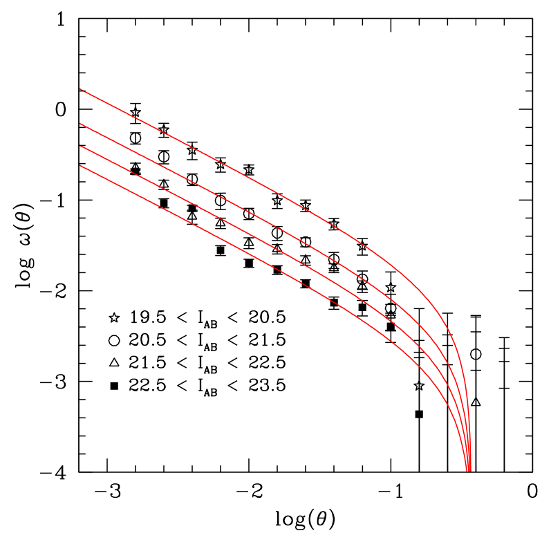
Figure 22: $I_{AB}$-selected galaxy clustering. For each magnitude slice, we show the amplitude of the angular correlation function, $\omega(\theta)$ as a function of the logarithm of the angular separation in degrees, $\log(\theta)$. At each magnitude slice, we show the fitted correlation amplitude, including a correction for the integral constraint term.

In Figure 23 we show the amplitude of $\omega(\theta)$ at $1\arcmin$ (assuming a slope $\delta=-0.8$) a function $I_{AB}$ sample median magnitude for the same magnitude slices presented in Figure 22. The open symbols and stars show the measurements from the CFDF survey and Wilson (2003) respectively. The amplitude of $\omega(\theta)$ at $1\arcmin$ steadily decreases with limiting magnitude: moreover, all magnitude bins agree quite well with the literature measurements.

Figure 23: The amplitude of the angular correlation function at arcminute scales. The filled symbols show $\log A_{\omega}(1\arcmin)$ as a function of $I_{AB}$ limiting magnitude as measured in the CFH12K-VIRMOS deep field, assuming a power-law form for the galaxy angular correlation function $\omega(\theta)$ with slope of $\delta=-0.8$ (error bars shown represent only the error bars from the fitting program and do not indicate the true cosmic errors, which are likely to be larger). The open circles and stars show measurements from other recent wide-field surveys.

It has recently reported that CFH12K observations may be affected by scattered light. This effect originates from light reflecting from structures inside the camera/telescope assembly. It produces an additive correction which is not removed by flat-fielding, as the flat-fields themselves are not uniformly illuminated. Measurements made at CFHT (and described extensively on the ELIXIR web pages) show that object magnitudes measured in the outer edges of the field of view can be as much 0.1 magnitudes fainter than in the central region.

We have looked for possible signatures of this problem in our catalogues. At large angular scales, the stellar correlation function we measure (Section 4.6) is consistent with zero (Figure 21). However, because the slope of the stellar number counts is relatively shallow compared to the galaxy counts (Section 4.3) the radial dependence of stellar counts will be comparatively weaker (corresponding to density changes of around a few percent). For galaxies, the steeper count slope means that the radial density dependence is higher, and so would be easier to detect this with a correlation function analysis as outlined above.

We used a scattered light image supplied by CFHT to investigate if the magnitude variation can have a significant effect on the measured $\omega(\theta)$. Because of the small dither offsets used in our observation strategy we are able to separate a single pointing from the four-pointing combined mosaic, and from this extracted sub-area we ’correct’ magnitudes in our catalogues based on the radial dependence derived at CFHT, and then re-apply our selected magnitude cuts. For galaxies with $18.5<I_{AB}<24.5$ we find that application of the scattered light map produces a difference of around $\sim 3.5\%$ in the total numbers of galaxies (below the systematic errors quoted in the previous sections). Furthermore, the measured $\omega(\theta)$ values computed at each angular separation do not differ significantly before and after the application of the scattered light correction (the difference is smaller than the Poissonian error bar in each bin). From these considerations, we conclude that the effects of residual scattered light in our catalogues is not detectable, at least to $I_{AB}<24.0$.

5 Summary

In this paper we have presented $BVRI$ optical data for the CFH12K-VIRMOS F02 deep field. Our observations reach limiting magnitudes of $B_{AB}\sim 26.5$, $V_{AB}\sim 26.2$, $R_{AB}\sim 25.9$ and $I_{AB}\sim 25.0$ (measured from our simulations). This field consists of a single contiguous area covering $1.2$ deg². In the magnitude range $18.0<I_{AB}<24.0$ there are 90,729 extended sources in our survey.

We have presented a detailed explanation of the reduction and preparation of the object catalogues and described how our astrometric and photometric solutions were computed. In summary, $68\%$ of catalogue sources have an absolute per co-ordinate residual less than $|\Delta\alpha|\sim 0.38\arcsec$ and $|\Delta\delta|\sim 0.32\arcsec$ in right ascension and declination respectively. Expressed in the same sense, our internal (filter-to-filter) per co-ordinate astrometric uncertainties are $|\Delta\alpha|\sim 0.08\arcsec$ and $|\Delta\delta|\sim 0.08\arcsec$. Our absolute photometric calibration, estimated from standard star data, and from galaxy number counts, is accurate to $\sim 0.1$ magnitudes. A series of Monte-Carlo simulations have been used to assess the reliability of catalogues in planes defined by peak surface brightness, position, and total magnitude. These show that our catalogues are reliable, uniform and fully complete to $I_{AB}<24.0$ .

Galaxy number counts in $BVRI$ bandpasses have been presented. We describe a method of star-galaxy separation which correctly accounts for the position-dependent seeing present in our final stacked images. Our galaxy counts are in good agreement with literature compilations, and our stellar counts are well matched by a theoretical model of the galaxy. Qualitatively, at each magnitude bin, $I_{AB}$ selected galaxy number counts in our survey agree to within $10\%$ with measurements made in the CFDF survey. Additionally, the slope of the galaxy counts in both $B$ and $I$ are consistent with previous determinations from other deep surveys. Furthermore, field galaxy colours in $(V-I)$ and $(B-V)$ measured in our survey are also in agreement (better than $0.1\leavevmode\nobreak\$mag) with measurements made in the Canada-France deep fields survey. The location of galaxies in colour-colour space, and its evolution with magnitude, is broadly consistent with expectations based on simple populations synthesis models.

We have also measured the angular correlation function of both stars and galaxies in our dataset. Stellar correlations are consistent with zero at all angular scales. Clustering of galaxies measured to $I_{AB-med}\sim 23$ in the angular range $-3<\log(\theta)<-1$ follows well the expected power law behaviour, and the observed scaling of the amplitude of $\omega(\theta)$ with $I_{AB-med}$ is in agreement with previous surveys. We have also investigated the possible effect that scattered light could have on the galaxy angular correlation function, and concluded that to $I_{AB}<24.0$ this effect does not pose a significant problem to our measurements.

Future papers will describe numerous extensions in wavelength to the survey field described here. Furthermore the catalogues presented in this paper are currently being used to select a very large magnitude-limited sample of objects for the VIRMOS-VLT deep survey. Together, both surveys will provide a unique picture of the Universe at intermediate and high redshifts.