New Dimensions in Cosmic Lensing

Andy Taylor

Institute for Astronomy, School of Physics, University of Edinburgh,

Royal Observatory Edinburgh, Blackford Hill,

Edinburgh, EH9 3HJ, U.K.

email: ant@roe.ac.uk

I review the current status of combing weak gravitational lensing with depth information from redshifts as a direct probe of dark matter and dark energy in the Universe. In particular I highlight: (1) The first maximum likelihood measurement of the cosmic shear power spectrum, with the COMBO17 dataset (Brown et al 2003); (2) A new method for mapping the 3-D dark matter distribution from weak shear, and its first application to the COMBO17 dataset (Taylor et al 2003); (3) A new method for measuring the Dark Energy of the Universe using purely the geometry of gravitational lensing, based on cross-correlation tomography (Jain & Taylor 2003). I show that this method can constrain the equation of state of the universe and its evolution to a few percent accuracy.

1 Introduction

Gravitational lensing provides us with the most direct and cleanest of methods for probing the distribution of matter in the universe (Mellier 1999, Bartelmann & Schneider 2001). The lensing effect arises due to the scattering of light by perturbations in the metric, stretching and contracting bundles of light rays, causing the distortion of background galaxy images. Hence gravitational lensing does not depend on any assumptions about the state of the intervening matter. These distortions manifest themselves as a shear distortion of the source galaxy image (see e.g. Tyson et al 1990; Kaiser & Squires 1993), or a change in the surface number density of source galaxies due to magnification (see e.g. Broadhurst, Taylor & Peacock 1995; Fort, Mellier & Dantel-Fort 1997; Taylor et al 1998) and can be used to map the two dimensional projected matter distribution of cosmological structure. As the matter content of the universe is dominated by non-baryonic and non-luminous matter, gravitational lensing is the most accurate method for probing the distribution of this dark matter.

Weak lensing studies have been carried out for a wide range of galaxy clusters, allowing precision measurements of cluster masses and mass distributions (see e.g. Tyson et al 1990, Kaiser & Squires 1993, Bonnet et al 1994, Squires et al 1996, Hoekstra et al 1998, Luppino & Kaiser 1997, Gray et al 2002). On larger scales, the shear due to large-scale structure has been accurately measured by several groups (see e.g. van Waerbeke et al 2001, Hoekstra et al 2002, Bacon et al 2002, Jarvis et al 2003, Brown et al 2003).

Depth information, from galaxy redshifts, has already been used in weak lensing studies to determine the median redshifts of the lens and background populations. This can be a limiting factor in the analysis, leaving uncertainty in the overall mass normalisation. In this review I describe an application using accurate shear and redshift information from the COMBO17 dataset (Wolf et al, 2003) to estimate the first maximum likelihood shear power spectrum analysis (Section 2), including all of the uncertainties associated with source distances (see Brown et al 2003). While the shear power contains much important information on the statistics of the dark matter distribution and cosmological parameters, a lot of information is projected out. However this is not a necessary step. In Section 3 I outline how the full 3-D dark matter distribution can be recovered from shear and redshift information, and make the first application to the COMBO17 data (see Taylor 2001, Bacon & Taylor 2003, Taylor et al 2003). Finally, in Section 4, I describe a new method for using shear and redshifts in a purely geometrical test to accurately measure the equation of state of the dark energy in the universe and its evolution (See Jain & Taylor 2003).

It is clear that the combination of shear and redshift information provides a powerful tool for cosmology, allowing us to not only image the dark matter directly, but also see its evolution over cosmic time. Hence future lensing surveys should consider being coupled to photometric redshift surveys, opening up new dimensions in gravitational lensing studies.

1.1 Basic weak lensing equations

The metric of a perturbed Robertson-Walker universe in the conformal Newtonian gauge is

$$ds^{2}=-(1+2\Phi)dt^{2}+a^{2}(t)(1-2\Phi)dr_{i}dr^{i},$$ (1)

where $\Phi$ is the Newtonian potential, $a$ is the cosmological scale factor, and we have assumed a spatially flat universe. The Newtonian potential is related to the matter density field by Poisson’s equation

$$\nabla^{2}\Phi=4\pi G\rho_{m}\delta a^{2}=\frac{3}{2}\lambda_{H}^{-2}\Omega_{m}a^{-1}\delta,$$ (2)

where $\delta=\delta\rho_{m}/\rho_{m}$ is the matter density perturbation, $\lambda_{H}=1/H_{0}\approx 3000\,h^{-1}{\rm Mpc}$ is the Hubble length, and $\Omega_{m}$ is the present-day mass-density parameter. The lensing potential, $\phi$, for a source in a spatially flat universe at a radial distance $r$ is given by (e.g. Bartelmann & Schneider 2001)

$$\phi(r,r\mbox{\boldmath$\theta$})=2\int_{0}^{r}\!\!dr^{\prime}\,\left(\frac{r-r^{\prime}}{rr^{\prime}}\right)\Phi(r^{\prime},r^{\prime}\mbox{\boldmath$\theta$}),$$ (3)

at an angular position $\theta$ on the sky. Hence the lensing potential is just a weighted radial projection of the 3-D gravitational potential.

In lensing the symmetric, tracefree shear matrix, $\gamma_{ij}$, which describes the distortion of the lensed image, and the magnification, $\mu$, which describes the change in area, are observables. The shear matrix is

$$\gamma_{ij}=\left(\partial_{i}\partial_{j}-\frac{1}{2}\delta^{K}_{ij}\partial^{2}\right)\phi,$$ (4)

where $\partial_{i}\equiv r(\delta_{ij}-\theta_{i}\theta_{j})\nabla_{j}=r(\nabla_{i}-\theta_{i}\partial_{r})$ is a dimensionless, transverse differential operator, and $\partial^{2}\equiv\partial_{i}\partial^{i}$ is the transverse Laplacian. The indices $(i,j)$ take the values $(1,2)$, assuming a flat sky. The lens convergence, $\kappa$, is defined by

$$\kappa=\frac{1}{2}\partial^{2}\phi.$$ (5)

An estimate of the lensing potential, $\widehat{\phi}$, can be found from the shear field by the Kaiser-Squires (1993) relation;

$$\widehat{\phi}(r,r\mbox{\boldmath$\theta$})=2\partial^{-4}\partial_{i}\partial_{j}\,\gamma_{ij}(r,r\mbox{\boldmath$\theta$}),$$ (6)

where $\partial^{-2}\equiv\int\!d^{2}\theta^{\prime}\,\ln|\mbox{\boldmath$\theta$}-\mbox{\boldmath$\theta$}^{\prime}|/2\pi$ is the inverse 2-D Laplacian operator. In practice the shear field is only discretely sampled by galaxies so we must smooth the shear field to perform the differentiation. This also serves to make the uncertainty on the measured shear field finite, since each source galaxy has an unknown intrinsic ellipticity. The scalar convergence field, $\kappa$, can be estimated from the shear field by combining equations (6) and (5), up to a constant of integration.

In principle there is another odd-party pseudoscalar which can be formed from a shear field;

$$\beta=\varepsilon^{m}_{i}\partial_{j}\partial_{m}\partial^{-2}\gamma_{ij},$$ (7)

where $\varepsilon^{i}_{j}$ is the 2-D antisymmetric Levi-Civita tensor. This field cannot correspond to the even-parity lens convergence field and can be used to investigate noise, boundary effects and intrinsic alignments of galaxies (Catelan, Kamionkowski & Blandford, 2001; Crittenden, et al 2001; Croft & Metzler, 2001; Heavens, Refregier & Heymans, 2000), which will appear in both $\kappa$ and $\beta$ modes. However, alignments appear to be a small effect at large redshift (Brown et al 2002, Heymans et al 2003).

2 The Shear Power Spectrum

2.1 Statistical properties

We may define a shear covariance matrix by

$$C_{ab}(\mbox{\boldmath$\theta$})=\langle\gamma_{a}(\mbox{\boldmath$0$})\gamma_{b}(\mbox{\boldmath$\theta$})\rangle,$$ (8)

where the indices $(a,b)$ each take the values (1,2). Fourier transforming the shear field,

$$\gamma_{ij}(\mbox{\boldmath$\ell$})=\int\!d^{2}\theta\,\gamma_{ij}(\mbox{\boldmath$\theta$})e^{-i\mbox{\boldmath$\ell$}.\mbox{\boldmath$\theta$}},$$ (9)

and decomposing it into $\kappa$ and $\beta$ we may generate the shear power spectra:

$$\langle\kappa(\mbox{\boldmath$\ell$})\kappa^{*}(\mbox{\boldmath$\ell$}^{\prime})\rangle = (2\pi)^{2}C^{\kappa\kappa}_{\ell}\delta_{D}(\mbox{\boldmath$\ell$}-\mbox{\boldmath$\ell$}^{\prime}),$$

$$\langle\beta(\mbox{\boldmath$\ell$})\beta^{*}(\mbox{\boldmath$\ell$}^{\prime})\rangle = (2\pi)^{2}C^{\beta\beta}_{\ell}\delta_{D}(\mbox{\boldmath$\ell$}-\mbox{\boldmath$\ell$}^{\prime}),$$

$$\langle\kappa(\mbox{\boldmath$\ell$})\beta^{*}(\mbox{\boldmath$\ell$}^{\prime})\rangle = (2\pi)^{2}C^{\kappa\beta}_{\ell}\delta_{D}(\mbox{\boldmath$\ell$}-\mbox{\boldmath$\ell$}^{\prime}).$$ (10)

The parity invariance of weak lensing suggests that $C^{\beta\beta}_{\ell}=C^{\kappa\beta}_{\ell}=0$. However other effects, such as noise and systematics, as well as intrinsic galaxy alignments may give rise to a non-zero $C^{\beta\beta}_{\ell}$. The cross-correlation of $\kappa(\ell)$ and $\beta(\ell)$ is expected to be zero but it allows a second check on noise and systematics in the shear field. In particular finite field and boundary effects can lead to leakage of power between these three spectra. The shear power spectrum and the convergence power are related by $C^{\gamma\gamma}_{\ell}=C^{\kappa\kappa}_{\ell}$ in the flat-sky approximation. For a spatially flat Universe, these are in turn related to the matter power spectrum, $P_{\delta}(k,r)$ by the integral relation (see e.g. Bartelmann & Schneider 2001):

$$C^{\kappa\kappa}_{\ell}=\frac{9}{4}\left(\frac{H_{0}}{c}\right)^{4}\Omega_{m}^{2}\,\int_{0}^{r_{\mathrm{H}}}\!dr\,P_{\delta}\left(\frac{\ell}{r},r\right)\left(\frac{\overline{W}(r)}{a(r)}\right)^{2},$$ (11)

where $a$ is the expansion factor and $r$ is comoving distance. $r_{\rm H}$ is the comoving distance to the horizon: $r_{\rm H}=c\int_{0}^{\infty}dz/H(z),$ where the Hubble parameter is given in terms of the matter density, $\Omega_{m}$, the vacuum energy density, $\Omega_{V}$ and the spatial curvature, $\Omega_{K}$ as $H(z)=H_{0}[(1+z)^{3}\Omega_{m}+(1+z)^{2}\Omega_{K}+\Omega_{V}]^{1/2}.$ The weighting, $\overline{W}$, is given in terms of the normalised source distribution, $G(r)dr=p(z)dz$:

$$\overline{W}(r)\equiv\int_{r}^{r_{\mathrm{H}}}\!dr^{\prime}\,G(r^{\prime})\,\frac{r^{\prime}-r}{r^{\prime}}.$$ (12)

The covariances of the shear field, equation (8), are related to the power spectra by (Hu & White 2001)

$$C_{11}(\hat{\mbox{\boldmath$r$}}) = \int\!\frac{d^{2}\ell}{(2\pi)^{2}}\,\big{(}C^{\kappa\kappa}_{\ell}\cos^{2}2\varphi_{\ell}+C^{\beta\beta}_{\ell}\sin^{2}2\varphi_{\ell}-C^{\kappa\beta}_{\ell}\sin 4\varphi_{\ell}\big{)}|W(\ell)|^{2}e^{i\mbox{\boldmath$\ell$}.\hat{\mbox{\boldmath$r$}}},$$

$$C_{22}(\hat{\mbox{\boldmath$r$}}) = \int\!\frac{d^{2}\ell}{(2\pi)^{2}}\,\big{(}C^{\kappa\kappa}_{\ell}\sin^{2}2\varphi_{\ell}+C^{\beta\beta}_{\ell}\cos^{2}2\varphi_{\ell}+C^{\kappa\beta}_{\ell}\sin 4\varphi_{\ell}\big{)}|W(\ell)|^{2}e^{i\mbox{\boldmath$\ell$}.\hat{\mbox{\boldmath$r$}}},$$

$$C_{12}(\hat{\mbox{\boldmath$r$}}) = \int\!\frac{d^{2}\ell}{(2\pi)^{2}}\,\big{(}\frac{1}{2}(C^{\kappa\kappa}_{\ell}-C^{\beta\beta}_{\ell})\sin 4\varphi_{\ell}+C^{\kappa\beta}_{\ell}\cos 4\varphi_{\ell}\big{)}|W(\ell)|^{2}e^{i\mbox{\boldmath$\ell$}.\hat{\mbox{\boldmath$r$}}},$$ (13)

where $\cos\varphi_{\ell}=\mbox{\boldmath$\hat{\ell}$}.\mbox{\boldmath$\hat{\ell}$}_{x}$ and $\mbox{\boldmath$\hat{\ell}$}_{x}$ is a fiducial wavenumber projected along the x-axis. We have included here a smoothing or pixelisation window function; $W(\mbox{\boldmath$\ell$})=j_{0}(\ell_{x}\theta_{\rm pix}/2)j_{0}(\ell_{y}\theta_{\rm pix}/2),$ where $j_{0}=\sin(x)/x$ is the zeroth order spherical Bessel function and $\theta_{\rm pix}$ is the smoothing/pixel scale.

With these relations, the three shear power spectra $C^{\kappa\kappa}_{\ell}$, $C^{\beta\beta}_{\ell}$ and $C^{\kappa\beta}_{\ell}$ can be estimated directly from shear data via a Maximum Likelihood approach (Hu & White 2001, Brown et al 2003). The dataset we have applied it to is the COMBO17 survey.

2.2 The COMBO17 Dataset

The data analysed is part of the COMBO-17 survey (Wolf et al. 2001), carried out with the Wide-Field Imager (WFI) at the MPG/ESO 2.2m telescope on La Silla, Chile. The survey currently consists of five $0.5^{\circ}\times 0.5^{\circ}$ fields totaling 1.25 square degrees with observations taken in five broad-band filters ($UBVRI$) and 12 narrow-band filters ranging from $420$ to $914$ nm. The chosen filter set facilitates accurate photometric redshift estimation ($\sigma_{z}\approx 0.05$) reliable down to an $R$-band magnitude of 24. During the observing runs the best seeing conditions were reserved for obtaining deep $R$-band images of the five fields to allow accurate weak lensing studies. It is these $R$-band images, along with the photometric redshift tables, that we make use of in this analysis. Gray et al (2002) discuss the procedure used to reduce the $R$ band imaging data, which totalled 6.3 hours. The imcat shear analysis package was applied to our reduced image (see Gray et al 2002 for details). This resulted in a catalogue of galaxies with centroids and shear estimates throughout our field, corrected for the effects of PSF circularization and anisotropic smearing. We appended to this catalogue the photometric redshifts estimated for each galaxy from the standard COMBO-17 analysis of the full multicolour dataset. Wolf et al (2002) describe in detail the photometric redshift estimation methods used to obtain typical accuracies of $\sigma_{z}=0.05$ for galaxies throughout $0<z<1$.

2.3 The COMBO17 shear power spectra

Figure 1: LHS: The total correlation function, $C(\theta)$, as measured from COMBO-17, along with the most recent cosmic shear measurements from the four other groups indicated. Beyond a scale of 1 arcmin, the measurements are in broad agreement. The correlation function predictions for a flat $\Lambda$CDM cosmology, for three values of the power spectrum normalisation (from top to bottom: $\sigma_{8}=1.0,0.9,0.8$) are also plotted. RHS: The cosmic shear power spectra from COMBO-17. Plotted on a linear-log scale are $C^{\kappa\kappa}_{\ell}$ (circles), $C^{\beta\beta}_{\ell}$ (crosses) and $C^{\kappa\beta}_{\ell}$ (triangles) in 5 band-averaged band powers, as a function of multipole, $\ell$, estimated from the optimal combination of a maximum likelihood analysis of the four COMBO-17 fields, CDFS, SGP, FDF, and S11. The error bars are estimated from the Fisher matrix. The solid curve is the shear power spectrum expected for a $\sigma_{8}=0.8$ normalised $\Lambda$CDM model. Once again, the $C^{\beta\beta}_{\ell}$ and $C^{\kappa\beta}_{\ell}$ points have been slightly horizontally displaced for clarity (from Brown et al 2003)

To compare our data with other surveys we have estimated the shear correlation function, $C(\theta)$, from COMBO17 and compared these with the results of other surveys. The results are shown in Figure 1 (LHS), where we see broad agreement with other surveys.

Fig. 1 (RHS) shows the COMBO17 shear power from a Maximum Likelihood analysis of the fields. Details of the analysis are given in Brown et al (2003). Three of our five band power measurements agree within their error bars with the $\sigma_{8}=0.8$ normalised $\Lambda$CDM model plotted. The high level of power measured at $\ell\sim 4000$ seems to be present in each of the fields we have analysed. The largest discrepancy between the model and the measurements occurs at $\ell=2000$ where less than half the power is found. We can check our results for systematic effects by estimating the power in the $\beta$-$\beta$ modes, as well as the $\kappa$-$\beta$ cross correlation. In all of our band powers the $\beta$-$\beta$ correlation is below the detected signal in $\kappa$ and is consistent with zero in all but one band power at $\ell\sim 4000$. Similarly the $\kappa$-$\beta$ cross correlation is well below our measurement of shear power, and is consistent with zero except at $\ell\sim 1000$ where a significant detection appears. We conclude from the minimal power found in these spectra that our results are not strongly contaminated by systematic effects. Subsequently we have used the photometric redshift information to remove close galaxy pairs to remove any intrinsic alignment effects (Heyman et al 2003). This had a negligible effect on our results, indicating that for current shear surveys this is not a major source of systematic.

2.3.1 Estimating $\Omega_{m}$ and $\sigma_{8}$

We are now in a position to use our measured shear power spectrum estimates to obtain a joint measurement of the normalisation of the mass power spectrum $\sigma_{8}$, and the matter density $\Omega_{m}$, by fitting theoretical shear correlation functions and power spectra, calculated for particular values of these parameters, to our measurements. Details are given in Brown et al (2003). Figure 2 shows the results of our parameter analysis in the $\sigma_{8}-\Omega_{m}$ plane (dark thin solid lines) for COMB017. A best-fit gives $\sigma_{8}=(0.72\pm 0.09)(\Omega_{m}/0.3)^{-0.49}$.

Figure 2: The likelihood surface of $\sigma_{8}$ and $\Omega_{m}$ from combining the COMBO-17 dataset with the 2dFGRS and pre-WMAP CMB constraints. The dark thin solid contours are the constraints obtained from our shear power spectrum analysis described in the previous section. The lighter vertical contours are the constraints on $\Omega_{m}$ obtained from the 2dFGRS where we have applied the priors described in the text to the 2dF data. The dashed set of contours are the constraints from a compilation of six pre-WMAP CMB experiments where we have assumed an optical depth to reionization of $\tau=0.10$. The dark heavy contours are the 1,2 and 3$\sigma$ combined constraints from the three methods. The best fit values of $\Omega_{m}$ and $\sigma_{8}$ are also indicated (from Brown et al 2003).

2.3.2 Combination with the 2dFGRS and Pre-WMAP CMB experiments

We can combine this confidence region with parameter estimations from other sources such as the 2dF Galaxy Redshift Survey (2dFGRS, Percival et al. 2002) and the various pre-WMAP CMB experiments (Lewis & Bridle 2002 & references therein). See Brown et al (2003) again for details of this combination. The results of this combination are shown in Figure 2 for an optical depth of $\tau=0.10$. Note that the 2dFGRS data we have used for this estimation constrains $\Omega_{m}$ only and so the constraints shown on $\sigma_{8}$ come wholly from the cosmic shear and CMB measurements. We measure best-fit values of $\Omega_{m}=0.27^{+0.02}_{-0.01}$ and $\sigma_{8}=0.73^{+0.06}_{-0.03}$ from the combined data. This compares well with the WMAP (+CBI, ACBAR, 2dFGRS and Lyman-$\alpha$ surveys) results of $\Omega_{m}=0.27\pm 0.04$ and $\sigma_{8}=0.84\pm 0.04$. Although there is some overlap in these surveys there does seem to be good convergence in these results. However to push to the even high accuracies we can expect in future lensing surveys, the main sources of systematics must be identified and removed.

3 Mapping the 3-D dark matter

While the cosmic shear signal, with an accurate knowledge of the source redshift distribution, provides an accurate probe of the projected dark matter component and cosmological parameters, the combination of shear and source redshifts contains much more information. Wittman et al (2001, 2002) have demonstrated the utility of using source redshifts by inferring a cluster redshift from shear and photometric redshift information for galaxies in their sample. The importance of redshift information to remove intrinsic galaxy alignments from shear studies has also been discussed by Heymans & Heavens (2002) and King & Schneider (2002a,b). Beyond this one would still like to image the full 3-D dark matter distribution over a large fraction of the Hubble volume. In particular this would aid seeing the cosmological growth of structure over cosmic time – something that can be calculated in the linear regime to high accuracy. In addition, while surveys such as WMAP have helped pin down cosmological parameter at high redshift, one would like to see them evolve. This is particularly important for parameters such as the equation of state of the universe, where its evolution can be used to distinguish between models for the dark energy. In fact it turns out that the 3-D mapping of dark matter is entirely feasible with good data. Here we outline the method proposed by Taylor (2001) and then an application to the COMBO17 data (see Taylor et al 2003). See also Hu & Keaton (2002) for a pixelised implementation to simulated data.

3.1 3-D reconstruction

Figure 3: Example of gravitational potential. Here we simulate the gravitational potential for two NFW clusters at ${\mathbf{r}}=(0.5,0.5,0.25)$ and $(0.5,0.7,0.4)$; the upper panel is a 3-D representation of ($y,z,\Phi$) resulting from an $x$ slice at $x=0.5^{\circ}$; the lower panel displays the $\Phi$ values for ($y,z$) in greyscale.

The inverse relation to equation (3) is

$$\Phi(r,r\mbox{\boldmath$\theta$})=\frac{1}{2}\partial_{r}r^{2}\partial_{r}\,\phi(r,r\mbox{\boldmath$\theta$}),$$ (14)

which can be verified by substitution into equation (3) and integrating by parts. Here the Newtonian potential is evaluated at the source position, and I assume the lensing potential is smooth enough to allow differentiation by the radial derivative $\partial_{r}=\mbox{\boldmath$\theta$}.\nabla$. The shear field provides an estimate of the lensing potential up to an arbitrary quadratic function;

$$\widehat{\phi}(r,r\mbox{\boldmath$\theta$})=\phi(r,r\mbox{\boldmath$\theta$})+\chi(r,\mbox{\boldmath$\theta$}),$$ (15)

where

$$\chi(r,\mbox{\boldmath$\theta$})=\psi(r)+\eta(r)\theta_{x}+\mu(r)\theta_{y}+\nu(r)(\theta_{x}^{2}+\theta_{y}^{2}),$$ (16)

is a solution to

$$\left(\partial_{i}\partial_{j}-\frac{1}{2}\delta^{K}_{ij}\partial^{2}\right)\chi(r,\mbox{\boldmath$\theta$})=0,$$ (17)

and $\psi$, $\eta$, $\mu$ and $\nu$ are arbitrary radial functions. This degeneracy is related to the so-called sheet-mass degeneracy which appears as a constant of integration, $4\nu$, when estimating the convergence from the shear field (Falco, Gorenstein & Shapiro 1985). However note that the degeneracy we find here will still appear, with $\nu=0$, even if the convergence field is used to estimate the lensing potential. These terms can be removed by taking moments of the measured lens potential over the area of a survey. Defining

$$\chi_{p,q}(r)=\frac{1}{A}\int_{A}\!d^{2}\theta\,\widehat{\phi}(r,r\mbox{\boldmath$\theta$})(\theta_{x}^{p}+\theta_{y}^{q}),$$ (18)

where $A$ is the area of a survey, an estimate of the lensing potential, with the mean, gradient and paraboloid contributions removed, is

$$\phi=\widehat{\phi}-\widehat{\chi}$$ (19)

where for a circular survey with radius $\Theta$,

$$\widehat{\chi}=4\chi_{0,0}\left(1-\frac{3\theta^{2}}{2\Theta^{2}}\right)-\frac{6\chi_{2,2}}{\Theta^{2}}\left(1-\frac{2\theta^{2}}{\Theta^{2}}\right)+\frac{2}{\Theta^{2}}\left(\chi_{1,0}\theta_{x}+\chi_{0,1}\theta_{y}\right),$$ (20)

assuming that the true potential averages to zero. Hence

$$\Phi(r,r\mbox{\boldmath$\theta$})=\frac{1}{2}\partial_{r}r^{2}\partial_{r}\left(\widehat{\phi}(r,r\mbox{\boldmath$\theta$})-\widehat{\chi}(r,\mbox{\boldmath$\theta$})\right)$$ (21)

is an estimate of the Newtonian gravitational potential, while

$$\delta(r,r\mbox{\boldmath$\theta$})=\frac{\lambda_{H}^{2}a}{3\Omega_{m}}\nabla^{2}\partial_{r}r^{2}\partial_{r}\left(\widehat{\phi}(r,r\mbox{\boldmath$\theta$}))-\widehat{\chi}(r,\mbox{\boldmath$\theta$})\right)$$ (22)

is an estimate of the density field. The derivation of equations (21) and (22) are the main results of this paper, and demonstrate that the full, 3-D Newtonian potential and density fields can be reconstructed from weak lensing observations. In practice $\chi$ will not be a major problem for large surveys where the moments of the true lensing potential will average to zero. However for small fields this may not be so true, and one may instead wish to set the edge of the field to $\phi=0$.

3.2 Simulations

Having set out the formal method for a 3-D reconstruction of the dark matter distribution, we now test it on simulations. Our simulation consists of a double cluster with a Navarro-Frenk-White profile (Figure 3). Further details can be found in Bacon and Taylor (2003).

3.3 Perfect dark matter reconstruction

Figure 4: Top panel: reconstructed gravitational potential using the full shear field of Figure 6, in a $100^{3}$ grid. This is a $(y,z)$ plane at $x=0.5^{\circ}$. Bottom panel: difference between input and recovered gravitational potential fields.

First we examine the accuracy of our method when the shear field is perfectly known everywhere. Figure 4 displays the reconstructed $\Phi$ and the difference between input and reconstructed fields. It can be seen that, with perfect knowledge of the shear field, a good reconstruction is achieved with our method. For the cluster at $z=0.25$, the error is $<0.4$% of the signal within a radius of 0.2 degrees of the cluster, except for the core pixel where the error is 11.5%. For the cluster at $z=0.5$, the error is $<5\%$ of the signal within a radius of 0.1 degrees of the cluster, except for the core pixel where the error is 17.6%. This is again due to the cusp at the cluster centre, which cannot be followed well by our averaged shear field. Nevertheless, it is clear that our method is successful in reconstructing cluster gravitational potentials in the absence of noise.

3.4 Realistic Dark Matter Reconstructions

Having demonstrated that the inversions of the shear field to obtain the gravitational potential is viable in the absence of noise, we now wish to add the two primary sources of noise present in lensing experiments: Poisson noise due to only sampling the field at a finite set of galaxy positions, and additional noise due to galaxies’ non-zero ellipticities. As an example we use number densities for plausible space-based experiments (100 per sq arcmin), and an appropriate number of objects at each redshift slice.

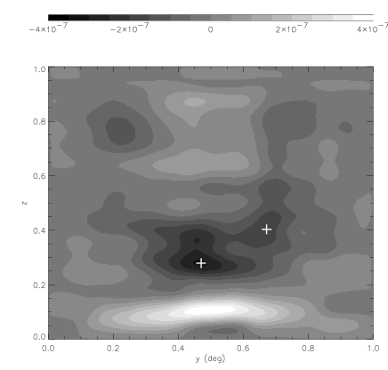
Figure 5: LHS Reconstructed dark matter potential for our space-based experiment, using galaxy properties as in Figure 9, after Wiener filtering. Note the detections of clusters at $(y,z)=(0.5,0.2)$ and $(0.7,0.4)$ with $\nu=4.2$ and 2.1 respectively (crosses show trough minima). RHS Cross-section in redshift and angles of the 3-D dark matter potential for the COMBO17 A901/2 supercluster field. Note that the lower large potential wells, at $z=0.2$, correspond to the A901/2 supercluster, and the higher potential well, at $z=0.4$, corresponds to an unknown background cluster.

Figure 5 (LHS) shows the dark matter potential measurements for our notional space-based survey after Wiener filtering. We measure the $z=0.25$ cluster with $\nu=4.2$ at the peak (trough) pixel of its gravitational potential well, with $\nu=2.1$ at the gravitational potential trough of the $z=0.4$ cluster. We also find a substantial noise peak in the foreground at $z=0.1$. While the recovery of the cluster gravitational potentials therefore constitutes a challenging measurement, we are indeed able to reconstruct useful information in the gravitational potential field itself. (The detection significance of these clusters is much higher than the measurement $\nu$ at a given point in the cluster).

3.5 Reconstructing the Dark Matter Potential in COMBO17

In this section, we will use these methods to calculate the dark matter potential for the COMBO17 supercluster A901/2 (See Gray et al 2002 for a 2-D shear analysis). For more details of the 3-D dark matter reconstruction see Taylor et al (2003).

Fig. 5 (RHS) shows a cross-section through the final $\Phi$ field. Note several significant features of this field. Firstly, we see that the gravitational potential trough associated with supercluster at $z=0.16$ is clearly recovered at the bottom of the plot, with a peak pixel S/N of 2.9. Secondly, further analysis shows that the gravitational potential displays troughs at approximately the positions of the three component clusters of A901/2. Thirdly, we note that a second mass concentration is measured at $z\simeq 0.4$, higher up in the plot. This has a peak pixel S/N of 2.8, so is certainly significant.

While the signal-to-noise on this ground-based application of the 3-D reconstruction is low, this clearly demonstrates the method. With higher numbers of sources in space-based surveys, we can expect to map out the dark matter distribution in 3-D over a significant fraction of the Hubble volume. Such 3-D dark matter catalogues can then be used as the basis for constructing mass-selected cluster catalogues with no projection effects.

4 Dark Energy from Lens Tomography

While the combination of shear and redshift information can be use to directly map the 3-D dark matter, an orthogonal application can also be made to probe the dark energy component of the Universe. The dark energy makes itself felt via its effect on the evolution of the universe and in particular the Hubble parameter, $H(a)$. This effects both the evolution of dark matter, and the geometry of the Universe. This effect has been utilised by, for example, Hu (2002), Huterer (2002), Abazajian & Dodelson (2002), Heavens (2003), Refregier et al (2003), Knox (2003) and Linder & Jenkins (2003).

Recently Jain & Taylor (2003) have proposed a new method based purely on the geometric effect of dark energy on gravitational lensing. This involves a particularly simple cross-correlation statistic: the average tangential shear around massive foreground halos associated with galaxy groups and galaxy clusters. We show that cross-correlation tomography measures ratios of angular diameter distances over a range of redshifts. The distances are given by integrals of the expansion rate, which in turn depends on the equation of state of the dark energy. Thus the lensing tomography we propose can constrain the evolution of dark energy. Lens tomography has also been studied as a valuable means of introducing redshift information into shear power spectra as a general method for improving parameter estimation (see e.g. Seljak 1998, Hu 1999, 2002, Huterer 2002, King & Schneider 2002b).

4.1 Method

The dark energy has equation of state $p=w\rho$, with $w=-1$ corresponding to a cosmological constant. The Hubble parameter $H(a)$ is given by

$$H(a)=H_{0}\left[\Omega_{m}a^{-3}+\Omega_{\rm de}e^{-3\int_{1}^{a}d\ln a^{\prime}(1+w(a^{\prime}))}\right]^{1\over 2},$$ (23)

where $H_{0}$ is the Hubble parameter today. The comoving distance is $r(a)=\int_{0}^{a}da^{\prime}/a^{\prime 2}H(a^{\prime})$.

We consider the lensing induced cross-correlation between massive foreground halos, which are traced by galaxies, and the tangential shear with respect to the halo center (denoted here $\gamma$): $\omega_{\times}(\theta)\equiv\left<\delta n_{\rm f}(\mbox{\boldmath$\theta$})\gamma(\mbox{\boldmath$\theta$}^{\prime})\right>$ where $n_{\rm f}(\mbox{\boldmath$\theta$})$ is the number density of foreground galaxies with mean redshift $\langle z_{\rm f}\rangle$, observed in the direction $\theta$ in the sky and $\delta n_{\rm f}(\mbox{\boldmath$\theta$})\equiv(n_{\rm f}(\mbox{\boldmath$\theta$})-{\bar{n}_{\rm f}})/{\bar{n}_{\rm f}}$. The angle between directions $\theta$ and $\mbox{\boldmath$\theta$}^{\prime}$ is $\theta$. The cross-correlation is given by (Moessner & Jain 1998, Guzik & Seljak 2002):

$$\omega_{\times}(\theta)=6\pi^{2}\Omega_{m}\int_{0}^{r_{H}}drW_{\rm f}(r)\frac{g(r,r_{b})}{a(r)}\int_{0}^{\infty}dk\,k\,P_{\rm hm}(r,k)\,J_{\mu}\left[kr\theta\right]\;,$$ (24)

where $g(r)$ is the lensing geometry averaged over the normalized distribution of background galaxies $W_{\rm b}(\chi)$

$$g(r)=r\int_{r}^{r_{H}}\!dr^{\prime}\,{r^{\prime}-r\over r^{\prime}}W_{\rm b}(r^{\prime})\ ,$$ (25)

$P_{\rm hm}(r,k)$ is the halo-mass cross-power spectrum, and $W_{\rm f}$ is the foreground halo redshift distribution. The Bessel function $J_{\mu}$ has subscript $\mu=2$ for the tangential shear and $\mu=0$ for the convergence. The measurement of the mean tangential shear around foreground galaxies is called galaxy-galaxy lensing. We will consider a generalization of this to massive halos that span galaxy groups and clusters. If the foreground sample has a narrow redshift distribution centered at $r=r_{\rm f}$, then we can take $W_{\rm f}$ to be a Dirac-delta function and evaluate the integral over $r$. All terms except $g(r_{\rm f},r_{\rm b})$ are then functions of $r_{\rm f}$, the redshift of the lensing mass. The coupling of the foreground and background distributions is contained solely in $g(r_{\rm f},r_{\rm b})$. Hence if we take the ratio of the cross-correlation for two background populations with mean redshifts $z_{1}$ and $z_{2}$, we get

$$\frac{\omega_{\times,1}(\theta)}{\omega_{\times,2}(\theta)}=\frac{g_{1}(r_{\rm f})}{g_{2}(r_{\rm f})}\approx\frac{(r_{1}-r_{\rm f})/r_{1}}{(r_{2}-r_{\rm f})/r_{2}},$$ (26)

where $w_{1},g_{1}$ denote the values of the functions for the background population with mean redshift $z_{1}$, and the second approximation is in the limit that the background galaxies also have a delta-function distribution. The above equations show that the change in the cross-correlation with background redshift does not depend on the galaxy-mass power spectrum, nor on $\theta$. We can simply use measurements over a range of $\theta$ to estimate the distance ratio of equation (26) for each pair of foreground-background redshifts. The distance ratio in turn depends on the cosmological parameters $\Omega_{\rm de}$, $w$, and its evolution $w^{\prime}$.

4.2 Signal-to-noise estimate

A simple way to estimate the signal-to-noise for the cross-correlation approach is to regard the foreground galaxies as providing a template for the shear fields of the background galaxies. For a perfect template (i.e. for high density of foreground galaxies and no biasing), the errors are solely due to the finite intrinsic ellipticities of background galaxies. Thus the fractional error in our measurement of the background shears is simply

$$\frac{\delta\gamma}{\gamma}\sim\frac{\sigma_{\epsilon}}{\sqrt{N_{\rm total}}\langle\gamma\rangle_{\rm rms}}\sim 0.2\times 10^{-3}\left(\frac{100}{n_{g}}\right)^{1/2}\left(\frac{0.1}{f_{\rm sky}}\right)^{1/2},$$ (27)

where the total number of background galaxies is $N_{\rm total}=n_{g}A=n_{g}f_{\rm sky}A_{\rm sky}$, $A$ is the survey area, the lensing induced rms shear $\langle\gamma\rangle_{\rm rms}\simeq 0.04$, the intrinsic ellipticity dispersion $\sigma_{\epsilon}=0.3$, and where the number density $n_{g}$ has units per square arcminute. Thus for the fiducial parameters $f_{\rm sky}=0.1$ and $n_{g}=100$, one can expect to measure the background shear to 0.1% accuracy at about 5-$\sigma$. We find that such a signal corresponds to changes in $w$ of a few percent; hence this is the approximate sensitivity we expect in the absence of systematic errors.

4.3 Dark energy parameters

Figure 6: Contours in the $\Omega_{\rm de}-w$ plane for the fiducial lensing survey with $f_{\rm sky}=0.1$. The inner contour assumes no evolution of dark energy, $w_{a}=0$, while the two outer contours marginalize over $w_{a}$, with external constraints on $\Omega_{v}$ corresponding to $\sigma(\Omega_{v})=0.01,0.03$ (see text). The $68\%$ confidence interval is shown in each of the contours. Contours in the $w-w^{\prime}$ plane for the fiducial lensing survey with $f_{\rm sky}=0.1$, as in Figure 6. The inner contour assumes $\Omega_{v}=0.7$, while the outer two contours marginalize over $\Omega_{v}$ as in Figure 6. Note that the parameter $w_{a}=2\ w^{\prime}$ at $z=1$ (from Jain & Taylor 2003).

We perform a $\chi^{2}$ minimization over the mean shear amplitudes at the two background distributions for each foreground slice to fit for the dark energy parameters. The time dependence of $w$ is parameterized as $w=w_{0}+w_{a}(1-a)$ (Linder 2002). For comparison with other work we will compare $w_{a}$ to $w^{\prime}$ defined by $w=w_{0}+w^{\prime}z$. Since the $w^{\prime}$ parameterization is unsuitable for the large redshift range we use, any comparison with it can be made only for a choice of redshift. For example, at $z=1$, which is well probed by our method and is of interest in discriminating dark energy models (Linder 2002), $w_{a}=2w^{\prime}$. For foreground slices labeled by index $l$ and two background samples by $1$ and $2$, the $\chi^{2}$ is given by

$$\chi^{2}=\sum_{l}\left[1-\frac{R^{0}(z_{l},z_{1},z_{2})}{R(z_{l},z_{1},z_{2})}\right]^{2}U_{l},$$ (28)

where $R$ is the distance ratio of equation (26) for given values of $\Omega_{v},w$ and $w_{a}$, and $R^{0}$ is the fiducial model with $\Omega_{v}=0.7,w=-1,w_{a}=0$. The weights $U_{l}$ are given by

$$U^{-1}_{l}=\frac{\sigma_{\epsilon}^{2}}{2n_{1}f_{l}A\ \langle\gamma\rangle^{2}_{l1}}+\frac{\sigma_{\epsilon}^{2}}{2n_{2}f_{l}A\ \langle\gamma\rangle^{2}_{l2}},$$ (29)

where $f_{l}$ is the fraction of the survey area $A$ covered by halo apertures in the $l$-th lens slice. The factor of $2$ in the denominator arises because we are using only one component of the measured ellipticity whereas $\sigma_{\epsilon}^{2}$ denotes the sum of the variances of both components.

The results are shown in Figures 6. Figure 6 (LHS) shows the constraints in the $\Omega_{v}-w$ plane. The ellipses show the $68\%$ confidence region given by $\Delta\chi^{2}=2.3$. The elongated inner contour is for fixed $w_{a}=0$. The two outer contours marginalize over $w_{a}$ assuming external constraints on $\Omega_{v}$ from the CMB and other probes, corresponding to $\sigma(\Omega_{v})=0.01,0.03$.

Figure 6 (RHS) shows the constraints in the $w-w_{a}$ plane if $\Omega_{v}$ is fixed, or marginalized over with $\sigma(\Omega_{v})=0.01,0.03$. The corresponding accuracy on $w$ and $w^{\prime}$ can be scaled as $f_{\rm sky}^{-1/2}$. For the case with $\sigma(\Omega_{v})=0.03$, we obtain $\sigma(w)\simeq 0.01f_{\rm sky}^{-1/2}$ and $\sigma(w_{a})\simeq 0.06f_{\rm sky}^{-1/2}$ (at $z=1$ this is equivalent to $\sigma(w^{\prime})\simeq 0.03f_{\rm sky}^{-1/2}$). Note that the value of $\sigma$ on a parameter is given by projecting the $\Delta\chi^{2}=1$ contour on the parameter axis, which is smaller than the projection of the inner contour in Figure 6 (RHS) with $\Delta\chi^{2}=2.3$. The scaling with $f_{\rm sky}$ in the parameter errors comes from the number of background galaxies (not sample variance), hence for given $f_{\rm sky}$ varying the depth of the survey scales the errors roughly as $n_{g}^{-1/2}$. The results we have shown are for the fiducial redshift $z=0$. A different choice of the fiducial redshift changes the relative accuracy on $w$ and $w_{a}$ somewhat, because the degeneracy direction in the three parameters changes. A detailed exploration of different models of $w(a)$ with finer bins in the background redshift distribution would be of interest.

5 Summary

In this paper I have presented three ways of combining weak lens shear data with source depth information. Firstly, one can use shear and redshifts to tie down the positions of source galaxies and remove this as a source of uncertainty in the measurement of the shear power spectrum. We have demonstrated this with an application to the COMBO17 dataset (Brown et al 2003). Secondly, with source redshifts I have demonstrated on simulations and with the COMBO17data, that the full 3-D dark matter distribution can be mapped (Taylor et al 2003). And finally with source redshifts the effect of the dark energy component of the universe can be explored via its effect on the geometry of gravitational lensing by taking ratios of cross-correlations of lens and source galaxies (Jain & Taylor 2003). Clearly, from these applications and many more, the availability of source redshifts has opened up a whole new dimension for gravitational lensing.

References

Abazajian K.N., Dodelson S., 2002, astro-ph/0212216.

Bacon D., Massey R., Refregier A., Ellis R.S., 2002, submitted to MNRAS, astro-ph 0203134.

Bacon D., Taylor A.N., 2003, MNRAS in press (astro-ph/0212266)

Bartelmann M., Schneider P., 2001, Phys. Rep., 340, 291.

Bonnet H., Mellier Y., Fort B., 1994, ApJL, 427, 83.

Broadhurst T., Taylor A.N., Peacock J., 1995, ApJ, 438, 49.

Brown M. L., Taylor A. N., Hambly N. C., Dye S., 2002, MNRAS, 333, 501

Brown M.L., Taylor A.N., Bacon D., Gray M., Dye S., Meisenheimer K., Wolf C., 2003, MNRAS, 341, 100

Catelan P., Kamionkowski M., Blandford R. D., 2001, MNRAS, 323, 713

Crittenden R., Natarajan P., Pen U., Theuns, T., 2001, ApJ, 545, 561

Croft. R. A. C., Metzler C. A., 2001, ApJ, 545, 561

Falco E.E., Gorenstein M.V. & Shapiro I.I., 1985, ApJLett, 289, L1

Fort B., Mellier Y., Dantel-Fort M., 1997, A&A, 321, 353

Gray M. E., Taylor A. N., Meisenheimer K., Dye S., Wolf C., Thommes E., 2002, ApJ, 568, 141.

Guzik J., Seljak U., 2002, MNRAS, 335, 311.

Heavens A. F., 2003, submitted to MNRAS, astro-ph/0304151

Heavens A. F., Refregier A., Heymans C., 2000, MNRAS, 319, 649

Heymans C., Heavens A. F., 2003, MNRAS, 339, 711

Heymans C., Brown M., Heavens A.F., Meisenheimer K., Taylor A.N., C. Wolf, 2003, submitted MNRAS

Hoekstra H., Franx M., Kuijken K., Squires G., 1998, ApJ, 504, 636.

Hoekstra H., Yee H., Gladders M., Barrientos L. F., Hall P., Infante L., 2002, ApJ, 575, 55.

Hu W., 1999, ApJL, 522, 21.

Hu W., 2002, Phys.Rev.D, 66, 083515

Hu W., White M., 2001, ApJ, 554, 67 (HW)

Hu W., Keeton C. R., 2002, submitted to PRD, astro-ph 0205412.

Huterer D., 2002, PRD, 65, 063001

Jain B., Taylor A.N., 2003, submitted to PRL, astro-ph/0306046

Jarvis M., Bernstein G., Jain B., Fischer P., Smith D., Tyson J.A., Wittman D., 2003, ApJ, 125, 1014

Kaiser N., Squires G., 1993, ApJ, 404, 441.

King L., Schneider P., 2002a, accepted by A&A, astro-ph 0208256.

King L., Schneider P., 2002b, A&A in press, astro-ph 0209474.

Knox L., 2003, astro-ph/0304370.

Lewis A., Bridle S., 2002, Phys. Rev. D., 66, 103511

Linder E.V., arXiv:astro-ph/0210217.

Linder E.V. & Jenkins A., 2003, astro-ph/0305286.

Luppino G. A., Kaiser N., 1997, ApJ, 475, 20.

Mellier Y., 1999, ARA&A, 37, 127

Moessner R., Jain B., 1998, MNRAS, 294, L18

Percival W. J. et al., 2002, MNRAS, 337, 1068

Refregier A., et al., 2003, astro-ph/0304419.

Squires G., Kaiser N., Fahlman G., Babul A., Woods D., 1996, ApJ, 469, 73.

Seljak U., 1998, ApJ, 506, 64.

Taylor A.N., et al, 1998, ApJ, 501, 539

Taylor A.N., 2001, Phys. Rev. Lett, submitted (astro-ph 0111605)

Taylor A.N., Bacon D.J., Gray M.E., Wolf C., Meisenheimer K., Dye S., 2003, submitted MNRAS

Tyson J.A., Valdes F., Wenk R.A., 1990, ApJLett, 349, L1

van Waerbeke L., Mellier Y., Radovich M., Bertin E., Dantel-Fort M., McCracken H. J., Le Fevre O., Foucaud S., Cuillandre J.-C., Erben T., Jain B., Schneider P., Bernardeau F., Fort B., 2001, A&A, 374, 757. y

Wittman D.M., et al, 2001, ApJ, 557, 89

Wolf C., Dye S., Kleinheinrich M., Rix H.-W., Meisenheimer K., Wisotzki L., 2001, A&A, 377, 442

Wolf C., Meisenheimer K., Rix H.-W., Borch A., Dye S., Kleinheinrich M., 2003, A&A, 401, 73