Structure of Dark Matter Halos From Hierarchical Clustering.
III. Shallowing of The Inner Cusp

Abstract

We investigate the structure of the dark matter halo formed in the cold dark matter scenarios by N-body simulations with parallel treecode on GRAPE cluster systems. We simulated 8 halos with the mass of $4.4\times 10^{14}M_{\odot}$ to $1.6\times 10^{15}M_{\odot}$ in the SCDM and LCDM model using up to 30 million particles. With the resolution of our simulations, the density profile is reliable down to 0.2 percent of the virial radius. Our results show that the slope of inner cusp within 1 percent virial radius is shallower than $-1.5$, and the radius where the shallowing starts exhibits run-to-run variation, which means the innermost profile is not universal.

1 Introduction

Since the ”finding” of the universal profile by Navarro, Frenk, and White (1996, 1997, hereafter NFW), the structure of dark matter halos formed through dissipationless hierarchical clustering from cosmological initial setting has been explored by many researchers. NFW performed a number of $N$-body simulations of the halo formation using 10-20k particles and found that the profile of dark matter halo could be fitted to a simple formula (hereafter, NFW profile)

$$\rho={\rho_{0}\over(r/r_{0})(1+r/r_{0})^{2}}$$ (1)

where $\rho_{0}$ is a characteristic density and $r_{0}$ is a scale radius. They also argued that the profile has the same shape, independent of the halo mass, the power spectrum of the initial density fluctuation or other cosmological parameters.

Several groups reported the results of similar simulations with much higher resolutions. However, disagreement concerning the inner structure still remains. Some researchers claimed that the slope of the inner cusp is steeper than that in the NFW’s results. Fukushige and Makino (1997) performed a similar simulation with 768k particles and found that the galaxy-sized halo has a cusp steeper than $\rho\propto r^{-1}$. Moore et al. (1998, 1999 hereafter M99) and Ghigna et al. (2000) performed simulations with up to 4M particles and obtained the results that the profile has a cusp proportional to $r^{-1.5}$ both in galaxy-sized and cluster-sized halos. M99 proposed the modified universal profile (hereafter, M99 profile),

$$\rho={\rho_{0}\over(r/r_{\rm 0})^{1.5}[1+(r/r_{\rm 0})^{1.5}]}.$$ (2)

Fukushige and Makino (2001, Paper I; 2003, Paper II) performed two series of $N$-body simulations, and found that the halos have density cusps proportional to $r^{-1.5}$, independent of the halo mass and cosmological models.

On the other hands, other researchers obtained the slope of inner cusp shallower than $-1.5$ and close to that in the NFW profile. Jing and Suto (2000, 2002) performed a series of $N$-body simulations and concluded that the power of the cusp depends on mass. It varies from $-1.5$ for galaxy mass halo to $-1.1$ for cluster mass halo. Klypin et al. (2001) obtained the slope at the center that could be approximated by $r^{-1.5}$. They, however, argued that the NFW fit is still good up to their resolution limit. Power et al. (2003) simulated an LCDM galaxy-sized halo with 3M particles and claimed that their circular velocity profile obtained is in better agreement with the NFW profile than with the M99 profile.

The purpose of this paper is to explore the inner structure of the dark matter halo by means of $N$-body simulations with about 10 times higher mass resolution than that of previous simulations. We simulated the formation of 8 cluster-sized halos in the SCDM and LCDM models using parallel Barnes-Hut treecode on parallel GRAPE cluster.

The structure of this paper is as follows. In section 2, we describe the model of our $N$-body simulation. In section 3, we present the results of simulation. Section 4 is for conclusion and discussion.

2 Simulation Method

We consider two cosmological models, SCDM model ($\Omega_{0}=1.0$, $h=0.5$, $\sigma_{8}=0.6$) and LCDM model ($\Omega_{0}=0.3$, $\lambda_{0}=0.7$, $h=0.7$, $\sigma_{8}=1.0$). Here, $\Omega_{0}$ is the density parameter, $\lambda_{0}$ is the dimensionless cosmological constant, and $H_{0}=100h\,{\rm km/s}\cdot{\rm Mpc}^{-1}$ at the present epoch. The amplitudes of the power spectrum in CDM models are normalized using the top-hat filtered mass variance at $8h^{-1}$ Mpc according to the cluster abundance (Kitayama & Suto 1997).

We simulate the formation of the dark matter halos using the ”re-simulation” method, which has been a standard method for the simulation of halo formation since NFW (1996). The procedure for setting the initial condition of halos are the same as that used in Paper II.

We first performed large scale cosmological simulations with $3.7\times 10^{6}$ particles in a sphere of 300$h$Mpc comoving radius. We regard spherical overdensity regions around local potential minima within $r_{\rm v}$ as candidate halos. We define the radius $r_{\rm v}$ such that the spherical overdensity inside is 178$\Omega_{0}^{0.3}$ times the critical density for SCDM and 178$\Omega_{0}^{0.4}$ times for LCDM model (Eke, Cole, Frenk 1998).

We selected 8 halos from the catalog of candidate halos. The selected halos are summarized in Table 1. We selected the three most massive halos and one halo randomly from halo candidates lying within 200$h$Mpc from the center in both models (so that the external tidal field can be included). We express a region within $5r_{v}$ from the center of the halo at $z=0$ in the cosmological simulation with larger number of particles. We place particles whose mass is as same as that in the cosmological simulation in a sphere of $\sim$ 100$h$Mpc comoving radius surrounding the high resolution region, in order to express the external tidal field. The total number of particles, $N$, is listed in Table 1. The generation of initial density fluctuation were done on HITACHI SR8000 (1 node) in Information Technology Center, University of Tokyo using COSMICS2 package (Bertschinger 2001).

Table 1: Run Properties

Model	Run	$M_{\rm v}$($M_{\odot}$)	$r_{\rm v}$ (Mpc)	$N_{\rm v}(\times 10^{6})$	$N(\times 10^{6})$	$m$ ($10^{7}M_{\odot}$)	$1+z_{i}$
SCDM	S1	$1.58\times 10^{15}$	3.08	29.2	60.3	5.39	44.2
	S2	$1.21\times 10^{15}$	2.84	31.2	60.7	3.86	45.5
	S3	$1.21\times 10^{15}$	2.84	4.5	10.0	26.5	37.9
	S4	$4.47\times 10^{14}$	2.03	6.9	13.9	6.46	43.4
LCDM	L1	$9.61\times 10^{14}$	2.43	25.2	62.8	3.80	51.1
	L2	$6.96\times 10^{14}$	2.20	26.0	59.9	2.67	52.7
	L3	$6.49\times 10^{14}$	2.15	7.2	16.7	9.01	47.5
	L4	$4.45\times 10^{14}$	1.88	7.8	13.5	5.67	49.4

We integrate the system directly in the physical coordinates for both the cosmological and halo simulations. We used a leap-flog integrator with shared and constant timestep. The step size for the cosmological simulation is $\Delta t/(t_{\rm H}-t_{\rm i})=1/1024$ and that for the halo simulation is $1/4096$. Here, $t_{\rm H}$ is the Hubble time and $t_{\rm i}$ is the time at which the simulation starts. The gravitational softening is constant in the physical coordinates and the length $\varepsilon_{\rm grav}$ is 5kpc for the cosmological simulation, and 1kpc for Runs S1, S2, L1, and L2, and 2kpc for other runs of halo simulations.

The force calculation is done with the parallel Barnes-Hut tree code on GRAPE clusters (Kawai, Makino 2003). GRAPE is a special-purpose computer designed to accelerate $N$-body simulations. The parallelization scheme we used are basically the same as Warren & Salmon’s (1993) Hashed Oct-Tree algorithm, except that we incorporated Barnes’ (1990) modified algorithm. The modification is necessary in order to make GRAPE work efficiently (Makino 1991). We use only the dipole expansion and the opening parameter $\theta=0.4$ for the cosmological simulation and $\theta=0.5$ for the halo simulation.

For high-resolution halo simulations, we used both a parallel GRAPE-5 cluster at University of Tokyo and a parallel MDGRAPE-2 cluster at RIKEN. The parallel GRAPE-5 cluster consists of 8 host computers (Pentium 4/1.9GHz, i845) each of which has one GRAPE-5 (Kawai et al. 2000) board. The parallel MDGRAPE-2 cluster consists of 8 host computers (Pentium4/2.2GHz, i850) each of which has one MDGRAPE-2 (Susukita et al. 2003) board. For cosmological simulations we used one board GRAPE-5. The simulation presented below needs, for example in Run S2, $\sim 300$ seconds per timestep, and thus one run (4096 timesteps) is completed in 350 hours (wallclock time) with the GRAPE-5 cluster.

3 Results

3.1 Snapshots

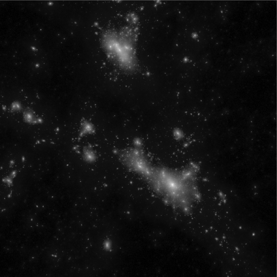
Figure 1: Snapplots from Run S2 at $z=0.58$. The length of the side is equal to 6.67Mpc.

Figure 1 shows the particle distribution for Run S2 at $z=0.58$ and $0$. The length of the side for each panel is 6.67 Mpc. For these plots, we shifted the origin of coordinates to the position of the potential minimum. In Table 1, we summarized the radius $r_{\rm v}$, the mass $M_{\rm v}$, and the number of particles $N_{\rm v}$ within $r_{\rm v}$ at $z=0$.

3.2 Density Profile

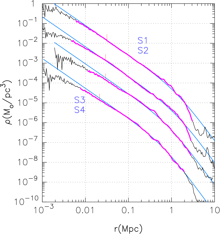
Figure 3: Density profile of the halos for all runs of the SCDM model at $z=0$. Only the densities plotted in the thick lines (colored magenta in online edition) satisfy criterion (3) in section 3.2 at $r<r_{\rm v}$. The labels indicate the run name. The profiles except for Run S1 are vertically shifted downward by 1, 2, 3 dex for Runs S2, S3, and S4, respectively. The vertical bar above the profiles indicate $0.01r_{\rm v}$. The solid curves (colored blue) indicate the density profile given by equation (2) (M99 profile).

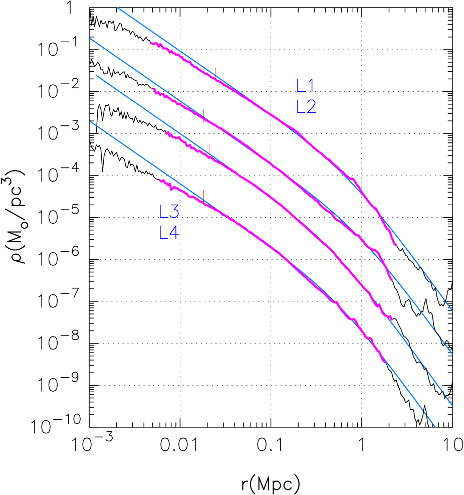
Figure 4: Same as Figure 3, but for the LCDM model.

Figures 3 and 4 show the density profiles of all runs at $z=0$ for SCDM and LCDM models, respectively. The exception is Run L4, for which we plot the density profile at $z=0.06$ because the merging process occurs just near the center of halos at $z=0$. The position of the center of the halo was determined using the potential minimum and the density was averaged over each spherical shell whose width is $\log_{10}(\Delta r)=0.0172$. For the illustrative purpose, the densities are shifted vertically.

We plot the densities by the thick (colored magenta in online edition) lines only if the criteria for two-body relaxation introduced in Paper I, $t_{\rm rel}(r)/t>3$, is satisfied, where $t_{\rm rel}(r)$ is the local two-body relaxation time given by

$$t_{\rm rel}={0.065v^{3}\over G^{2}\rho m\ln(R_{\rm max}/\varepsilon)},$$ (3)

(cf. Spitzer 1987) and $R_{\rm max}$ is a maximum impact parameter. Here we set $R_{\rm max}$ to 1 Mpc as a system size. We also confirmed that other numerical artifacts due to the time integration did not influence the density profile as will be discussed in section 3.3.2. The potential softening does not influence the profile since the reliability limit obtained by the above criterion is more than three times larger than the softening length for all runs.

At $r>0.02$ Mpc or $r>0.01r_{\rm v}$, the density profiles are in good agreement to the profile given by equation (2) (the M99 profile) in all runs. This result is consistent with the previous simulations performed with a few million particles (M99, Ghigna et al. 2000, Paper I, Paper II). The fitting here was done using $M_{\rm v}$ and the least square fit of $(\rho-\rho_{\rm M99})/\rho_{\rm M99}$ at $0.03<r<0.5$ Mpc. The scale radii $r_{0}$ obtained by the fitting are summarized in Table 2.

Table 2: Fitting Parameters

Run	$r_{0}$ (Mpc)	$r_{0}$ (Mpc)	$r_{0}$ (Mpc)	$r_{\rm c}$ (Mpc)	$r_{\rm v}$ (Mpc)
	for $\rho_{\rm M99}$	for $\rho_{\rm NFW}$	for $\rho_{\rm n1}$	for $\rho_{\rm n2}$
S1	1.36	0.41	0.70	0.0014	3.05
S2	1.31	0.40	0.68	0.0014	2.82
S3	0.88	0.42	0.60	0.0036	2.82
S4	0.66	0.29	0.44	0.0023	1.97
L1	0.75	0.31	0.50	0.0023	2.40
L2	0.95	0.33	0.52	0.0015	2.13
L3	0.48	0.23	0.34	0.0027	2.13
L4	0.57	0.26	0.38	0.0024	1.82

On the other hands, at $r<0.01r_{\rm v}$, we can see the shallowing of the cusp from the power $-1.5$ for all run. The degree of the shallowing seems to increase as the radius decreases, which seemingly suggests that the inner cusp profile does not converge to a single slope. Moreover, the point where the profile starts to depart from the $r^{-1.5}$ cusp is different for different runs. For example, in Run S1 the departure starts at $\sim 0.005r_{\rm v}$, while at $\sim 0.02r_{\rm v}$ in Run L3. This means that the density profile is not universal.

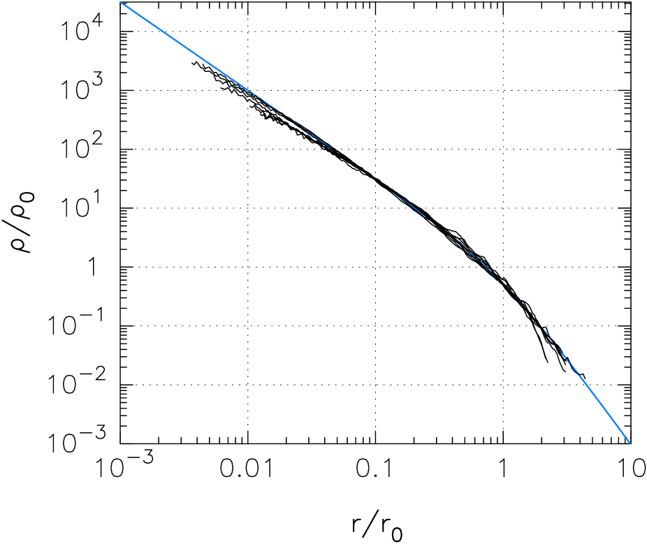
Figure 5: Density profiles for all runs scaled by $r_{0}$ and $\rho_{0}$ (Table 2). The solid (colored blue in online edition) curves indicates the density profile given by equation (2) (M99 profile).

In Figure 5 we plot the density profiles for all runs scaled by $r_{0}$ and $\rho_{0}$, together with the M99 profile. We can see that at $r/r_{0}<0.05$ all profiles are systematically shallower than the $r^{-1.5}$ cusp, and that in this region run-to-run variation of the profile is significant. On the other hands, at $r/r_{0}>0.05$ the profiles are in good agreement with M99 profile. Although there are some dispersion from M99 profile at $r/r_{0}>0.3$, they are not systematic.

3.3 Reliability

3.3.1 Two-body relaxation

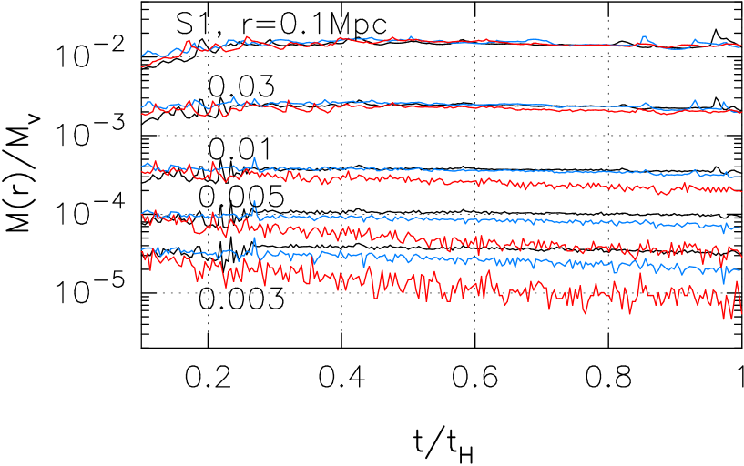
Figure 6: Cumulative mass within radii, 0.1, 0.03, 0.01, 0.005, and 0.003 Mpc, as a function of time, for three simulations with 29(Run S1, thick lines), 14(intermediate thick, colored blue in online edition) and 1 (thin, colored red) million particles.

Figure 7: Density profiles for three simulations with 29(Run S1, thick lines), 14(intermediate thick, colored blue in online edition) and 1 (thin, colored red) million particles. The vertical bars indicate the reliability limits obtained by criterion (3) in section 3.2.

We test the reliability of the criterion (3)using the simulations of the same initial condition as used in Run S1 but with several different values for the total number of particles ($N$). Except for $N$, we used the same simulation parameters as in Run S1. Figure 7 show the cumulative mass $M_{\rm r}(r)$ within the radii, 0.1, 0.03, 0.01, 0.005, and 0.003 Mpc, as a function of time, for three simulations with 29(Run S1), 14 and 1 million particles within $r_{\rm v}$. Figure 7 shows the final density profiles for three simulations. The vertical bars indicates the reliability limit obtained by the criterion (3).

In Figure 7, we can see that the cumulative mass evolution obtained in the simulations with 29 and 14 millions particle are in good agreement for $r>0.01$ Mpc. This agreement indicates that our criterion (0.009 Mpc for 14 millions particle run) gives a good reliability limit. In Figure 7 we can also see that the density $\rho$ obtained in the simulations with 29 and 14 millions particle are in good agreement outside the reliability limit of 14 millions particle run (0.009 Mpc). The agreement of the averaged density is somewhat worse than that of the density. This is because the averaged density is integrated quantity. Any error of the density inside the sphere of radius $r$ affects the average density at radius $r$.

Recently, Power et al. (2003) proposed another reliability criterion for the two-body relaxation, given by

$${t_{\rm rel}(r)\over t}=\displaystyle{{N(r)\over 8\ln{N(r)}}\left({\rho_{\rm ave}\over 200\rho_{\rm crit}}\right)^{-1/2}}>0.6.$$ (4)

Although their function form is different from ours and ignores the dependence on potential softening (see, Fig 3 of Paper I), it gives reliability limits similar to ours. For example, in Run S1, the reliability limit given by their criterion is 0.007, 0.009 and 0.025 Mpc for simulations with 29, 14 and 1 millions particles. These values are within 15% of our limit shown in Figure 7.

3.3.2 Time integration

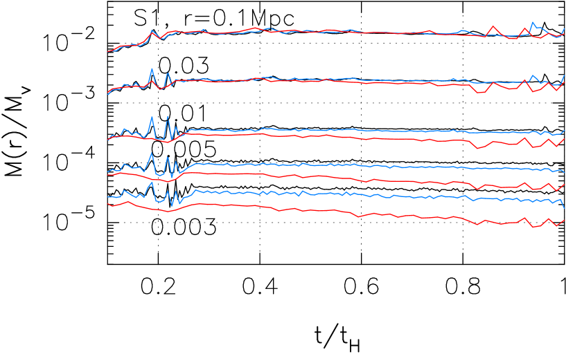
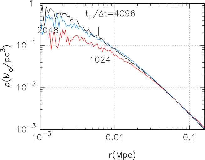
Figure 8: Same as Figure 7, but for for three simulations with $\Delta t/(t_{\rm H}-t_{\rm i})=$1/4096(Run S1, thick lines) , 1/2048(intermediate thick, colored blue in online edition) and 1/1024(thin, colored red).

Figure 9: Density profiles for three simulations with $\Delta t/(t_{\rm H}-t_{\rm i})=$1/4096 (Run S1, thick lines), 1/2048(intermediate thick, colored blue in online edition) and 1/1024(colored red). The vertical bars indicate the reliability limits obtained by criterion (3) in section 3.2.

If the stepsize for the time integration is too large, it also influences the profile. We check whether the stepsize of time integration used in our simulations is small enough by performing the simulations from the same initial model as Run S1 but with several different stepsize ($\Delta t$). Except for $\Delta t$, we used the same simulation parameters as in Run S1. Figure 9 show the cumulative mass within the radii, 0.1, 0.03, 0.01, 0.005, and 0.003 Mpc, as a function of time for three simulations with $\Delta t/(t_{\rm H}-t_{\rm i})=$1/4096(Run S1), 1/2048 and 1/1024. Figure 9 show the profile of the density $\rho$ for three simulations at $t/(t_{\rm H}-t_{\rm i})=0.78125$. We plot the profile at this time since, in the simulation with $\Delta t/(t_{\rm H}-t_{\rm i})=$1/2048, merging process occurs near the center of halos at around $z=0$.

In these figures we can see that larger stepsize makes the central profile shallower. The density profile outside of 0.007 Mpc converges even by adapting 1/2048. Therefore, we can conclude that the stepsize of $\Delta t/(t_{\rm H}-t_{\rm i})=$1/4096 did not introduce any numerical artifact.

Power et al. (2003) investigated influences of the large stepsize on the profile, and showed that the influence depends also on the softening length. They found that if potential softening length is larger than an optimal length, $\varepsilon\simeq 4r_{\rm v}/\sqrt{N_{\rm v}}$, a reliability limit is given by

$${t_{\rm c}(r)\over t_{\rm c}(r_{\rm v})}=15\displaystyle{\left({\Delta t\over t_{0}}\right)^{5/6}},$$ (5)

and if softening length is smaller than the optical length more timesteps are required than that given by criterion (5).

However, an application of Power et al. (2003)’s criterion to our simulation results seems to give unphysically reliability limits. For example, in Run S1, the reliability limit given by criterion (5) is 0.016, 0.038 and 0.083 Mpc for simulations with 1/4096, 1/2048 and 1/1024, respectively. From Figure 9, it is clear that these values are far too large. Although we do not fully understand the origin of the difference, such difference is possible. The error in time integration is very complicated because it depends not only on the stepsize and softening length, as Power et al. (2003) showed, but also on the integration scheme selected (ex. variable timestep or not, in comoving space or in physical space).

3.4 Fitting by NFW profile

In Figure 10, we fit the density profiles for all runs to the NFW profile. The fitting here was done using $M_{\rm v}$ and the least square fit of $(\rho-\rho_{\rm NFW})/\rho_{\rm NFW}$ at $r<0.5$ Mpc (down to the reliability limit). The scale radii $r_{0}$ obtained by the fitting are summarized in Table 2. We can see that the NFW profile is not in good agreement with simulation results, except for Run L3. Figure 11 show the residual, $(\rho-\rho_{\rm NFW})/\rho_{\rm NFW}$, together with that for the M99 profile. The agreement with the NFW profile is not good in all radii, while that with the M99 profile is not good only in inner region ($r<0.03$Mpc). Moreover, we can see that the sign of the residuals for NFW profile systematically change, which means the central slope of the NFW profile is too shallower.

3.5 Evolution

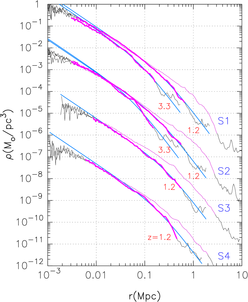
Figure 12: Evolution of density profile for all runs of the SCDM model. The numbers near profiles indicate the redshift. The profiles at $z=0$ are plotted by the thin lines. Only the densities plotted in the thick (colored magenta in online edition) lines satisfy criterion (3) in section 3.2 at $r<r_{\rm v}$. The solid curves (colored blue) indicate the density profile given by equation (2) (M99 profile).

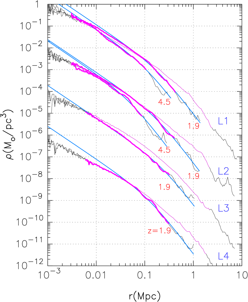
Figure 13: Same as Figure 12, but for the LCDM model.

Figures 12 and 13 show the growth of the density profile for all runs. The virial radii and the masses within the virial radius at the redshift plotted are summarized in Table 3. We fit these profiles to the M99 profile. The fitting procedure is as same as that for Figure 3. The scale radii $r_{0}$ obtained by the fitting are summarized in Table 3.

Table 3: Parameters at higher redshift

Run	$z$	$r_{\rm v}$ (Mpc)	$M_{\rm v}$ ($M_{\odot}$)	$r_{0}$(Mpc)
S1	3.3	0.16	$1.9\times 10^{13}$	0.085
	1.2	0.65	$1.6\times 10^{14}$	0.25
S2	3.3	0.15	$1.6\times 10^{13}$	0.056
	1.2	0.55	$9.7\times 10^{13}$	0.20
S3	1.2	0.55	$9.8\times 10^{13}$	0.29
S4	1.2	0.46	$5.5\times 10^{13}$	0.20
L1	4.5	0.11	$1.4\times 10^{13}$	0.11
	1.9	0.42	$1.2\times 10^{14}$	0.20
L2	4.5	0.086	$7.3\times 10^{12}$	0.05
	1.9	0.40	$7.0\times 10^{13}$	0.18
L3	1.9	0.32	$5.4\times 10^{13}$	0.24
L4	1.9	0.31	$4.7\times 10^{13}$	0.13

At the inner region ($r<0.03$ Mpc), we can see the density keeps almost unchanged from relatively higher redshift for all runs. This fact also can be seen in the evolution of the cumulative mass shown in Figure 7. This means that the density at the inner region is determined by that of the smaller halo that collapsed at higher redshift.

The density profile of the outer region is formed as the halo grows and shows universality. Moreover, the agreement with the M99 profile at higher redshift is very well down to the radius at which the cusp shallowing can be seen at $z=0$, independent of the cosmological model we simulated in this paper. Figure 14 shows the relation between the scale radius $r_{0}$ and density $\rho_{0}$ obtained by the fitting. We can see clearly an evolutionary pass along a line, $\rho_{0}\propto r_{0}^{-1.5}$, also independent of the cosmological model.

3.6 Different Fitting

In section 3.2, we see that the agreement with the M99 profile is not good at the inner region ($r<0.02$Mpc), and also that with the NFW profile is worse in the whole range of profile in section 3.4. Therefore, it is worthwhile to fit the results to other profiles. Here, we try to fit the results to two different profiles.

Firstly, we fit the results to a profile that has an inner cusp shallower than that of the M99 profile and steeper than the NFW profile [fitting (1)], given as

$$\rho_{\rm n1}=\displaystyle{\rho_{0}\over(r/r_{\rm 0})^{\alpha}\left[1+(r/r_{\rm 0})^{3-\alpha}\right]}$$ (6)

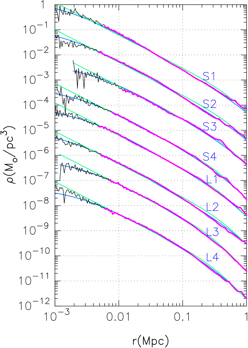
Figure 15: Density profiles for all runs at the inner region. The solid curves indicate the density profiles given by equations (6) (colored green in online edition) and (7) (colored blue).

where $\alpha$ is the power of the inner cusp and we set $\alpha=1.3$. In Figure 15, we fit the density profiles to the profile given by equation (6). The fitting here was done using $M_{\rm v}$ and the least square fit of $(\rho-\rho_{\rm n1})/\rho_{\rm n1}$ for $r<0.5$ Mpc (down to the reliability limit). The scale radii $r_{\rm 0}$ obtained by the fitting are summarized in Table 2. Figure 16 shows the residual $(\rho-\rho_{\rm n1})/\rho_{\rm n1}$. The agreement is better than both the M99 and NFW profiles.

We also tried to add another power law region ($\propto r^{\beta}$) to the M99 profile [fitting (2)], given as

$$\rho_{\rm n2}=\displaystyle{\rho_{0}\over C_{0}(r/r_{\rm c})^{\beta}\left[1+(r/r_{\rm c})\right]^{1.5-\beta}\left[1+(r/r_{\rm 0})^{1.5}\right]}$$ (7)

where

$${1/C_{0}}=(r_{0}/r_{\rm c})^{\beta}\left[1+r_{0}/r_{\rm c}\right]^{1.5-\beta},$$ (8)

$r_{\rm c}$ is another scale radius. Although this profile includes more parameters to fit, it is based on the observation that two different mechanisms might be working in the growth of the halo as suggested by the analyses in section 3.5.

In Figure 15, we fit the density profiles to the profile given by equation (7). Here, for simplicity, we set $\beta=0$ for all runs and, therefore, the equation (7) becomes

$$\rho_{\rm n2}=\displaystyle{\rho_{0}\over C_{0}\left[1+(r/r_{\rm c})\right]^{1.5}\left[1+(r/r_{\rm 0})^{1.5}\right]}$$ (9)

where

$${1/C_{0}}=\left[1+(r_{0}/r_{\rm c})\right]^{1.5}$$ (10)

The fitting here was done using $r_{0}$ obtained in the fitting to the M99 profile and the least square fit of $(\rho-\rho_{\rm n2})/\rho_{\rm n2}$ at $r<0.5$ Mpc. The scale radii $r_{\rm c}$ obtained are summarized in Table 2. Figure 16 shows the residual, $(\rho-\rho_{\rm n2})/\rho_{\rm n2}$. As a matter of course, agreement is better than that for any other profile, since we increased the number of fitting parameters.

Unfortunately, in the present simulations, the region that we can use to determine which fitting formula is more appropriate is not so large. Further studies with simulations with higher resolution and larger number of samples would be necessary.

4 Conclusion and Discussion

We performed $N$-body simulations of dark matter halo formation in SCDM and LCDM models. We simulated 8 halos whose mass range is $4.4\times 10^{14}M_{\odot}$ to $1.6\times 10^{15}M_{\odot}$ using up to 30 millions particles.

Our main conclusions are:

• We found that, in all runs, the slope of inner cusp within $0.01r_{\rm v}$ is shallower than $-1.5$, and the radius where the shallowing starts exhibits run-to-run variation, which means the profile is not universal.

• We found that the profile is in agreement with the M99 profile for $r>0.01r_{\rm v}$, and are not in agreement with the NFW profile. We present different fitting formulae to describe the whole range of the simulation results.

Although we found interesting features in the inner structure of dark matter halo by new simulations with much higher resolution, we could not achieve the final understanding of the structure. One question remained is whether the CDM halo has a flat core or not. Another question is whether the same shallowing can be seen in the halo of galaxy or dwarf galaxy size. The origin of the inner structure is also still unclear. In order to answer these questions, we are now planning to perform larger simulations using new GRAPE cluster system.

Figure 2: Same as Figure 1, but at $z=0$.

Figure 10: Density profiles for all runs. The solid curves (colored blue in online edition) indicate the density profile given by equation (1) (NFW profile).

Figure 11: Residuals $(\rho-\rho_{\rm M99})/\rho_{\rm M99}$ and $(\rho-\rho_{\rm NFW})/\rho_{\rm NFW}$ as a function of radius.

Figure 14: The scale density $\rho_{0}$ as a function of the scale radius $r_{0}$ (Table 3) at the redshift plotted in Figures 12 and 13. The dashed line indicates $\rho_{0}\propto r_{0}^{-1.5}$.

Figure 16: Residuals $(\rho-\rho_{\rm n1})/\rho_{\rm n1}$ and $(\rho-\rho_{\rm n2})/\rho_{\rm n2}$ as a function of radius.