INFLATION FROM BRANES AT ANGLES

Abstract

In this lecture I will review the present status of inflation within string-based brane-world scenarios. The idea is to start from a supersymmetric configuration with two parallel static Dp-branes, and slightly break the supersymmetry conditions to produce a very flat potential for the field that parametrises the distance between the branes, i.e. the inflaton field. This breaking can be achieved in various ways. I will describe one of the simplest examples described in Ref. [1]: two almost parallel D4-branes in a flat compactified space, with a small relative angle between the branes, softly breaking supersymmetry. If the breaking parameter is sufficiently small, a large number of $e$-folds can be produced within the D-brane, for small changes of the configuration in the compactified directions. Such a process is local, i.e. it does not depend very strongly on the compactification space nor on the initial conditions. Moreover, the breaking induces a very small velocity and acceleration, which ensures very small slow-roll parameters and thus an almost scale invariant spectrum of metric fluctuations, responsible for the observed temperature and polarization anisotropies in the microwave background. Another prediction of the model is the small amplitude of the gravitational wave spectrum, which could be undetectable in the near future. Inflation ends as in hybrid inflation, triggered by the negative curvature of the string tachyon potential.

1 Introduction

Inflation is a paradigm in search of a unique model, that may eventually be described within a complete theory of particle physics [2]. For the moment we just have the basics or fundamentals of inflation, and do not just have a single (definitive) realization of inflation, but many. So, how do we construct a consistent model of inflation within particle physics? First, we have to provide an effective scalar field, the inflaton; but what is the nature of this inflaton field? Then we have to give a dynamics for this field, some effective potential that is sufficiently flat for inflation to proceed; but how do we attain such flatness? Furthermore, the amplitude and tilt of (scalar and tensor) metric fluctuations should agree with the observed CMB temperature and polarization anisotropies, as well as the LSS matter distribution seen by deep galaxy redshift surveys. These observations suggest an approximately scale invariant spectrum of adiabatic Gaussian curvature perturbations with an amplitude of a few parts in $10^{5}$.

Over the years there have been a handful of particle physics candidates of inflation [3] based on a variety of concepts: a) symmetry breaking (to trigger the end of inflation), in models of hybrid inflation [4]; b) supersymmetry (in order to cancel dangerous polynomial loop corrections) which gives rise to reasonably flat directions like in D- or F-term inflation [3]; and c) string theory (in search of a consistent theory of gravity at the quantum level [5]), which generically gives slow-roll parameters of order one, and thus makes sufficient inflation difficult to realize.

Recently, the proposals of Refs. [6, 7, 8, 9, 10, 11, 12, 13] have managed to derive some of the inflationary properties from concrete non-supersymmetric stringy (brane) configurations. A new development started in the mid-nineties, within $d=10$ superstring theory, with the “discovery” of the D(p)-branes, i.e. non-perturbative extended (p+1)-dimensional objects on which fundamental strings could live and/or attach their ends to. In the presence of branes, strings can satisfy two distinct boundary conditions [5]:

$$\begin{array}[]{lr}{\rm Neumann:}&\left.X^{\mu}(\tau,\sigma)\right|_{\rm brane}=0\,,\\[5.69054pt] {\rm Dirichlet:}&\left.\partial_{\sigma}X^{\mu}(\tau,\sigma)\right|_{\rm brane}=0\,.\\ \end{array}$$ (1)

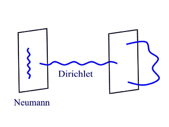
Figure 1: This figure represents two Dp-branes with strings living along the brane, satisfying Neumann boundary conditions, as well as open strings with both ends attached to one or two branes, satisfying Dirichlet boundary conditions.

These D-branes are dynamic objects, whose forces arise from the exchange of open and closed string modes between them. One can compute exactly (within string theory) the potential corresponding to the interaction between Dp-Dp or Dp-$\overline{\rm Dp}$ branes [5]. There are two possible types of modes exchanged between branes: Ramond-Ramond (R-R) modes (fermions, $C_{p}$-potentials) and Neveu-Schwarz-Neveu-Schwarz (NS-NS) modes (graviton, dilaton). When supersymmetry is preserved, the NS-NS and R-R charges cancel and there is no net force between the branes.

In that case, the 1-loop amplitude due to exchange of string modes cancels exactly, ${\cal A}_{\rm 1-loop}={\cal A}_{\rm NS-NS}-{\cal A}_{\rm R-R}=0$, where [5]

$${\cal A}_{\rm 1-loop}=2V_{p+1}\int_{0}^{\infty}{dt\over 2t}\int{d^{p+1}k\over(2\pi)^{p+1}}\left[\rm Tr{1+(-1)^{F}\over 2}\,e^{-2\pi t\,{\rm L}_{0}^{\rm(NS)}}-\rm Tr{1+(-1)^{F}\over 2}\,e^{-2\pi t\,{\rm L}_{0}^{\rm(R)}}\right]\,.$$ (2)

Thus, two parallel Dp-branes constitute a stable BPS state. The tree-level potential is solely determined by the sum of the branes’ tensions, $V_{0}=2T_{p}=$ constant, and therefore generates no force.

In this context, it was proposed by Dvali and Tye [6] the idea of brane inflation, in which the role of the inflaton field is played by the interbrane separation $y$. They treated the potential phenomenologically, without actually deriving it from string theory. Just assuming Gauss law for the massless modes propagating between branes, they wrote the potential at large distances as

$$V(y)\approx V_{0}-{B\over y^{d_{\bot}-2}}\,,$$ (3)

where $d_{\bot}=10-(p+1)$ is the number of compact dimensions transverse to the branes and $B$ is a certain coefficient, in principle derivable from string theory. With this potential, inflation occurs, but requires unnatural fine tuning of $B\ll 1$ in order to have sufficient number of $e$-folds .

One of the main interests of dealing with these non-perturbative objects in string theory is that they are extended objects of dimension (p+1) and, in principle, our (3+1) world could be embedded in them. If the forces between these objects give rise to effective potentials for certain scalars, one could then produce inflation within the branes, in the context of string theory, and thus explain our present homogeneity and flatness. This is what makes the scenario very attractive.

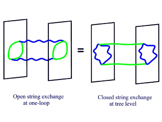
Figure 2: The interaction between two Dp-branes arise from the exchange of closed string modes at tree level, which is equivalent to the 1-loop exchange of open string modes.

2 Brane-antibrane inflation

Soon after the proposal of Dvali and Tye, two groups obtained independently an exact expression for $V(y)$ in the case of maximal supersymmetry breaking of the BPS, i.e. with a brane and an antibrane [8, 7]. Since the antibrane has opposite RR charges than the brane, the 1-loop amplitude does not vanish, ${\cal A}_{\rm 1-loop}={\cal A}_{\rm NS-NS}-{\cal A}_{\rm R-R}=2{\cal A}_{\rm NS-NS}\neq 0$, and thus there appears a force at 1-loop between the brane and the antibrane. Let us suppose for concreteness that the brane has dimension (3+1) like our own world, and thus consider a system of D3-$\overline{\rm D3}$ branes. Such branes have (3+1) dimensions which are Neumann with respect to the propagation of the strings embedded in them, and $d_{\bot}=6$ transverse compactified dimensions, which are assumed to be fixed somehow,  along which the bulk strings satisfy Dirichlet boundary conditions. An schematic view of this brane-antibrane system can be seen in Fig. 3. The branes are separated a certain distance apart in the compactified space, as represented by the crosses in the planes $(X_{4},\,X_{5}),\ (X_{6},\,X_{7}),\ (X_{8},\,X_{9})$.

Figure 3: This figure represents two D3-branes. The usual 4-dimensional spacetime is along directions $\{x^{0},...,x^{3}\}$. The branes are located at particular points on the remaining six compact directions $\{x^{4},...,x^{9}\}$.

At large distances, the 1-loop amplitude is dominated by the term

$${\cal A}_{\rm NS-NS}\propto G_{9-p}(y)\propto{1\over y^{d_{\bot}-2}}={1\over y^{4}}\,,$$ (4)

where $G_{9-p}(y)$ is the massless propagator in $(9-p)$ dimensions. As we will see, the proportionality constant depends on the string theory couplings and can be calculated explicitly.

On the other hand, at short distances, it is well known [5] that the low energy effective theory of the brane-antibrane system contains a tachyon whose mass squared becomes negative,

$$m_{T}^{2}={y^{2}\over 4\pi^{2}{\alpha^{\prime}}^{2}}-{1\over 2\alpha^{\prime}}\,,$$ (5)

below a certain distance $y\leq y_{c}=\sqrt{2\pi^{2}\alpha^{\prime}}\equiv\sqrt{2\pi^{2}}\ l_{s}$, of order the string scale. A tachyon signals the instability of the system and therefore the end of inflation. In fact, the behavior of the system is very similar to that of hybrid inflation [4]. It is probably the first example of the generic model of hybrid inflation in the context of string theory.

This simple model, however, has a fundamental flaw: after inflation, the brane-antibrane disappear completely (they mutually annihilate), radiating into the bulk, not along the brane, and thus would not produce the required reheating of the universe after inflation responsible for the subsequent stages of Big Bang cosmology. There are a few ways out, by including different types of branes of higher dimension which decay into lower-dimensional branes, see [8], or by adding extra degrees of freedom like electric or magnetic fluxes on the branes, which will prevent their complete annihilation.

In any case, this model does not produce enough inflation to solve the flatness and homogeneity problems. The reason is quite simple: superstring theory give coefficients and couplings that are of order one in string units, and therefore, the brane and antibrane attract eachother too strongly and collide before the brane-world has time to expand sufficiently to solve those problems. Let us see this explicitly for the case of D3-$\overline{\rm D3}$ branes [7, 8].

The 4-dimensional effective action for the interbrane separation $y$ is given by

$$S=\int d^{4}x\,\sqrt{-g}\left[{1\over 2}M_{P}^{2}\,R-{1\over 2}T_{3}\,(\partial y)^{2}-V(y)\right]\,,$$ (6)

where $T_{3}=M_{s}^{4}g_{s}^{-1}/(2\pi)^{3}$ is the D3-brane tension, and the 4-dimensional Planck mass is given by $M_{P}^{2}=M_{s}^{2}(M_{s}^{6}V_{6})g_{s}^{-2}$, with $V_{6}\equiv(2\pi R)^{6}$ the volume of the 6-dimensional compactified space (here assumed to be a 6-torus of common radius $R$). The effective potential for the inflaton can be obtained from string theory (for $p=3$), assuming that the distance between branes is large compared with the string scale but small compared with the compactified space ($l_{s}\ll y\ll 2\pi R$), as

$$V(y)=2T_{p}+4\pi(4\pi^{2}\alpha^{\prime})^{3-p}\,G_{9-p}(y)\equiv M^{4}\left(1-{\alpha\over\phi^{4}}\right)\,,$$ (7)

where $\phi\equiv T_{3}^{1/2}y$  is the canonically normalized inflaton field, and  $\alpha=M^{4}/32\pi^{2}$.

It is easy to compute the number of $e$-folds from this potential,

$$N={1\over M_{P}^{2}}\int{V\,d\phi\over V^{\prime}(\phi)}={2\pi^{2}\over 3(2\pi)^{6}}\,\left({y\over 2\pi R}\right)^{6}\,.$$ (8)

In the approximation in which this potential was computed, $y\ll 2\pi R$, the number of $e$-folds is much smaller than one and thus insufficient for solving the homogeneity and flatness problems. Put another way, in order to have enough number of $e$-folds , $N\simeq 60$, one would require $y>2\pi R$, and therefore, one would have to take into account the infinite series of images of the branes (and antibranes) in the compactified space. This was considered in Ref. [8] and found to give rise to an effective potential which could marginally provide enough number of $e$-folds , as long as the initial conditions of inflation were chosen very close to a symmetric configuration. We will not pursue this issue here, but will now describe an alternative and quite robust solution for brane inflation that we came up with in Ref. [1].

3 Inflation from branes at angles

In order to overcome the difficulties of constructing successful inflationary models from brane-antibrane interactions, where supersymmetry is maximally broken, we considered in Ref. [1] the possibility of generating the inflaton potential from the spontaneous breaking of supersymmetry, so that one can smoothly turn on an interaction between the branes. There are many ways in which this general idea can be implemented: by a slight rotation of the branes intersecting at small angles (equivalent, in the T-dual picture, to adding small magnetic fluxes through the branes), by considering small relative velocities between the branes, by introducing orientifolds, etc. In Ref. [1] we considered the interactions that arise between intersecting branes at a small angle. If the angle is small then supersymmetry is only slightly broken, so that the force between the branes is relatively small. It is this flat potential which will drive inflation, as the branes are attracted to each other, until a tachyonic instability develops when the branes are at short distances compared with the string scale. This is a signal that a more stable configuration with the same R-R total charge is available, which triggers the end of inflation.

In the following we elaborate on one of the simplest examples: a pair of D4-branes intersecting at a small angle in some compact directions [1]. The interaction can be arbitrarily weak by choosing the appropriate angle to be sufficiently small. The brane-antibrane system is the extreme supersymmetry breaking case, where the angle is maximised such that the orientation for one brane is opposite to the other. The interaction is so strong in this case, that inflation seems hard to realise [7]. One should take very particular initial conditions on the system for inflation to proceed [8]. On the other hand, if the supersymmetry breaking parameter is small, a huge number of $e$-folds are available within a small change of the internal configuration of the system, due to the almost flatness of the potential; in this way the initial conditions do not play an important role. Thus, we find that inflation is robust in systems that are not so far from supersymmetry preserving ones.

The following table gives us some perspective on the model building possibilities for inflation in the context of stringy brane constructions.

$\theta=0$	Brane-Brane (parallel)	SUSY preserved	No force (static) BPS
$\theta=\pi$	Brane-Antibrane (antiparallel)	maximal SUSY breaking	Large attractive force
$\theta\ll\pi$	Brane-Brane (small angle)	spontaneous SUSY breaking	Weak attractive force

The aim is to obtain an almost flat potential for the moduli field describing the interbrane separation. One of the interesting features of branes in string theory is that they can wrap around certain cycles in the compactified space. The wrapping has associated with it an angle $\theta$ and a length $L$, see Fig. 5. These parameters will characterize the inflaton potential.

4 Description of the model

In our paper [1], we considerd type IIA string theory on ${\cal R}^{3,1}\times T^{6}$, with $T^{6}$ a (squared) six torus. We put two D4-branes expanding 3+1 world-volume dimensions in ${\cal R}^{3,1}$, with their fourth spatial dimension wrapping some given 1-cycles of length $L$ on one of the $T^{2}$ in $T^{6}$. In Fig. 4 we have drawn a concrete configuration.

Figure 4: This figure represents two D4-branes at an angle $\theta$. The usual 4-dimensional spacetime is along directions $\{x^{0},...,x^{3}\}$. The branes are located at particular points on the four compact directions $\{x^{4},...,x^{7}\}$. Finally, they wrap different cycles on the last two compact directions, $x^{8}$ and $x^{9}$, and intersect at a given angle $\theta$.

If both branes are wrapped on the same cycle and with the same orientation, we have a completely parallel configuration that preserves sixteen supercharges, i.e. ${\cal N}=4$ from the 4-dimensional point of view. If they wrap the same cycle but with opposite orientations, we have a brane-antibrane configuration, where supersymmetry is completely broken at the string scale [23]. But for a generic configuration with topologically different cycles, there is a non-zero relative angle, let us call it $\theta$, in the range $0\leq\theta\leq\pi$, and the squared supersymmetry-breaking mass scale becomes proportional to $2\theta/(2\pi\alpha^{\prime})$, for small angles. The case we are considering can be understood as an intermediate case between the supersymmetric parallel branes ($\theta=0$) and the extreme brane-antibrane pair ($\theta=\pi$), with the angle playing the role of the smooth supersymmetry breaking parameter in units of the string length.

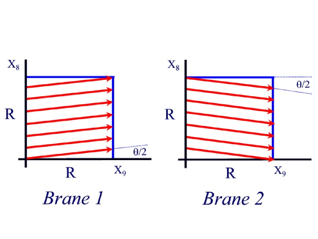
Figure 5: The wraping of the two D4-branes around the compactified space at an angle $\theta/2$ with opposite orientations. The relative angle between the two branes is $\theta$. If the branes wrap many times along one direction, the angle $\theta$ can be quite small.

Notice that this configuration does not satisfy the R-R tadpole conditions [24]. These conditions state that the sum of the homology cycles where the D-branes wrap must add up to zero. In our case these conditions do not play an important role, since we can take a brane, with the opposite total charge, far away in the transverse directions. This brane will act as an expectator during the dynamical evolution of the other two branes. Also, since the configuration is non-supersymmetric, there are uncancelled NS-NS tadpoles that should be taken into account [25, 26, 27, 5]. They act as a potential for the internal metric of the manifold, e.g. the complex structure of the last two torus in the 8-9 plane, and for the dilaton. Along this paper we will consider that the evolution of these closed string modes is much slower than the evolution of the open string modes.

Each brane is located at a given point in the two planes determined by the compact directions $\{x^{4},...,x^{7}\}$; let us call these points $y_{i}$, $i=1,2$. In the supersymmetric ($\theta=0$) configuration there is no force between the branes and they remain at rest. When $\theta\not=0$, a non-zero interacting force develops, attracting the branes towards each other. From the open string point of view, this force is due to a one-loop exchange of open strings between the two branes. The coordinate distance between the two branes in the compact space, $y^{2}=|y_{1}-y_{2}|^{2}$, plays the role of the inflaton field, whose vacuum energy drives inflation. At tree level, the vacuum energy is provided by the D4-brane tension $T_{4}$ and the brane length $L$ around the 1-cycle, $V_{0}=2\,T_{4}\,L$. At one loop, the potential is given by the zero-point vacuum energy,

$$V_{\rm 1-loop} = \sum_{i}\int{d^{3}k\over(2\pi)^{3}}\,{\hbar\omega_{k}^{i}\over 2}$$ (9)

$$= {1\over 64\pi^{2}}\sum_{i}(-1)^{F_{i}}\,m_{i}^{4}\,\ln m_{i}^{2}$$

$$= {-1\over(4\pi)^{2}}\int_{0}^{\infty}{dt\over t^{3}}\,\sum_{i}(-1)^{F_{i}}e^{-t\,m_{i}^{2}}$$ (10)

where the sum goes over all string states of mass $m_{i}$. This expression is nothing but the Coleman-Weinberg potential for the low energy effective field theory. The fact that $\sum_{i}(-1)^{F_{i}}\,m_{i}^{2n}=0,\ (n=1,2,3)$, ensures that (9) is finite, as it should be, since supersymmetry is being spontaneously broken.

We can now compute the full potential at 1-loop order, following Ref. [5]

$$V_{\rm 1-loop}(y_{i},\theta)=-\int_{0}^{\infty}{dt\over t}(8\pi^{2}\alpha^{\prime}\,t)^{-2}\sum_{n_{i}}e^{-{t\over 2\pi\alpha^{\prime}}\sum_{i}(y_{i}+n_{i}2\pi R_{i})^{2}}Z(\theta,t)\,,$$ (11)

which splits into three terms: The first term contains the integration over momenta in the (3+1) non-compact dimensions. The second term is the sum over winding modes in the compact transverse dimensions. For small distances $y$ compared with the size of the compactified space, it becomes

$$\sum_{n_{i}}e^{-{t\over 2\pi\alpha^{\prime}}\sum_{i}(y_{i}+n_{i}2\pi R_{i})^{2}}\ \stackrel{{\scriptstyle y_{i}\ll 2\pi R}}{{-\!\!\!-\!\!\!-\!\!\!\longrightarrow}}\ e^{-{t\,y^{2}\over 2\pi\alpha^{\prime}}}\,,$$ (12)

with $y^{2}=\sum_{i}y_{i}^{2}$ the coordinate distance between the branes in the compact space. Branes know about this space only through their winding modes. If the initial condition satisfies $y_{i}\ll 2\pi R$, the winding modes are so massive that they decouple. Once the branes start to fall towards eachother we can ignore the presence of the compact space thereafter. Of course, we will be assuming that the actual size ($R$) of the compact space becomes fixed by some yet unknown mechanism, and that the branes are thus free to move within this space.

The last term is the string partition function,

$$Z(\theta,t)={\Theta^{4}_{11}(i\theta t/2\pi,it)\over i\,\Theta_{11}(i\theta t/\pi,it)\,\eta^{9}(it)}\,,$$ (13)

which contains a sum over all open string modes propagating between the branes. The $\eta(\tau)$ and $\Theta_{11}$ are the Dedekind and the Jacobi elliptic functions that come from the bosonic and fermionic string modes, respectively.

At large distances compared with the string scale, $l_{s}\ll y\ll 2\pi R$, the terms dominating the integral in Eq. (11) come from the limit $t\to 0$,

$$Z(\theta,t)\ \stackrel{{\scriptstyle t\to 0}}{{\longrightarrow}}\ 4\,t^{3}\,\sin^{2}{\theta\over 2}\,\tan{\theta\over 2}\,.$$ (14)

The interbrane potential thus becomes

$$V(y,\theta)=V_{0}+V_{\rm 1-loop}=2\,T_{4}\,L-{\sin^{2}{\theta\over 2}\,\tan{\theta\over 2}\over 8\pi^{3}\alpha^{\prime}\,y^{2}}\,,$$ (15)

with $\theta\ll 1$ fixed. Therefore, the 4-dimensional action is given by

$$S=\int d^{4}x\,\sqrt{-g}\left[{1\over 2}M_{P}^{2}\,R-{1\over 2}T_{4}\,L\,(\partial y)^{2}-V(y)\right]\,,$$ (16)

with a Planck mass  $M_{P}^{2}=M_{s}^{2}(2\pi R\,M_{s})^{6}\,g_{s}^{-2}$. The canonically normalized field we will call the inflaton is  $\phi=(T_{4}\,L)^{1/2}\,y$, which has an effective potential at large distances given by

$$V(\phi) = M^{4}\left(1-\beta\,{M_{s}^{2}\over\phi^{2}}\right)\,,$$ (17)

$$M^{4} \equiv 2T_{4}\,L={M_{s}^{4}(M_{s}\,L)\,g_{s}^{-1}\over 32\pi^{4}}\,,$$ (18)

$$\beta \equiv {\sin^{2}{\theta\over 2}\,\tan{\theta\over 2}\over 16\pi^{3}}\simeq{\theta^{3}\over 128\pi^{3}}\ll 1\,.$$ (19)

This potential has the expected form, with the right power of the distance, as would arise from Gauss law.

At short distances, $y\leq l_{s}$, there is a string mode that acquires a negative mass squared, signalling the end of inflation through the tachyon condensation. If $\theta\neq 0$, there exists a non-trivial cycle that minimizes the volume, and hence the energy, of the system and the two branes become unstable, see Fig. 6.

Figure 6: Two D4-branes attract each other to decay in the last step to a bound state. Inflation will take place when the two branes are far away if the angle between the two branes is small enough. We have chosen here $\theta=\pi/2$ for pictorical purposes. In fact the branes are at an angle $\theta\ll 1$, so we would expect the final brane to be wrapped around the corresponding cycle.

From the low energy effective theory, it signals the appearance of the string tachyon, with mass

$$m_{T}^{2}={y^{2}\over 4\pi^{2}{\alpha^{\prime}}^{2}}-{\theta\over 2\pi\alpha^{\prime}}\,,$$ (20)

which defines the bifurcation point, $y=y_{c}=\sqrt{2\pi\theta}\ l_{s}$, below which the mass squared is negative $m_{T}^{2}<0$, and the tachyon triggers the end of inflation, in a way completely analogous to that which occurs in hybrid inflation [4], see Fig. 7.

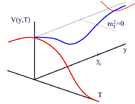
Figure 7: A sketch of the inflaton-tachyon potential $V(T,y)$. The flat region corresponds to the inflationary regime. The red lines correspond to the tachyon potential at large distances $y\gg y_{c}$, and at $y=0$. Note that it approaches asymptotically the tachyon vev at infinity.

5 Brane inflation

Let us now use the inflaton potential (17) to derive phenomenological bounds on the parameters of the model. Note that a small angle $\theta\ll\pi$ ensures $\beta\ll 1$ and therefore a flat potential. Also, $\theta\ll\pi$ implies $y_{c}\ll l_{s}$, so that we may have enough number of $e$-folds before the string tachyon triggers the end of inflation.

The number of $e$-folds and the slow-roll parameters can be computed as [2, 3, 32]

$$N = {1\over M_{P}^{2}}\,\int{V\,d\phi\over V^{\prime}(\phi)}={1\over 8\beta}\left({M_{s}^{2}\over M_{P}^{2}}\right)^{2}\,{\phi^{4}\over M_{s}^{4}}\gg 1\hskip 28.45274pt{\rm for}\ \beta\ll 1\,,$$ (21)

$$\epsilon = {M_{P}^{2}\over 2}\left({V^{\prime}(\phi)\over V(\phi)}\right)^{2}\simeq{1\over 32\,N^{2}}\,{\phi^{2}\over M_{s}^{2}}\ll 1\,,$$ (22)

$$\eta = M_{P}^{2}\,{V^{\prime\prime}(\phi)\over V(\phi)}=-\,{3\over 4N}\,,$$ (23)

$$\xi = M_{P}^{4}\,{V^{\prime}\,V^{\prime\prime\prime}(\phi)\over V^{2}(\phi)}={3\over 4N^{2}}\,.$$ (24)

Substituting $N\simeq 58$, we find the scalar tilt and its running as

$$n_{s} = 1+2\eta-6\epsilon\ \simeq\ 1-\,{3\over 2N}\simeq 0.974\,,$$ (25)

$${d\,n_{s}\over d\ln k} = -2\xi-{2\over 3}\Big{[}(n_{s}-1)^{2}-4\,\eta^{2}\Big{]}\ \simeq-\,{3\over 2N^{2}}\simeq-4\times 10^{-4}\,,$$ (26)

which constitute specific predictions, that should be compared with observations of the anisotropies of the microwave background. For the moment, COBE [33] and Boomerang [34], as well as the recent results of WMAP [35] seem to be in agreement with these predictions, at the 2$\sigma$ level. Furtheremore, the observed amplitude of temperature fluctuations fixes the size of the intersecting angle between branes,

$$\delta_{H} = {1\over 5\pi\sqrt{3}}{V^{3/2}\over V^{\prime}\,M_{P}^{3}}={N^{3/4}2^{-1/4}\over 5\sqrt{3}\pi^{3}}{g_{s}\,(M_{s}\,L)^{1/2}\over\beta^{1/4}(2\pi\,R\,M_{s})^{9/2}}=1.9\times 10^{-5}\,,$$ (27)

$$\beta^{1/4} = 3.3\times 10^{3}\,{g_{s}\,(M_{s}\,L)^{1/2}\over(2\pi\,R\,M_{s})^{9/2}}\,.$$ (28)

These constrain fix a few scales. For instance, the value of the inflaton field becomes

$${\phi_{*}\over M_{s}}=(2\beta N)^{1/4}\,(M_{s}\,2\pi R)^{3/2}\,g_{s}^{-1/2}=1.5\times 10^{4}\,{(M_{s}Lg_{s})^{1/2}\over(M_{s}\,2\pi R)^{3}}\,,$$ (29)

where the asterisc denotes the time when the present horizon-scale perturbation crossed the Hubble scale during inflation, 58 $e$-folds before the end on inflation. In terms of the distance between branes,

$${y_{*}\over l_{s}} = 4\pi^{2}\left({g_{s}\over M_{s}\,L}\right)^{1/2}{\phi_{*}\over M_{s}}=6\times 10^{5}\,{g_{s}\over(M_{s}\,2\pi R)^{3}}\,,$$ (30)

$${y_{*}\over 2\pi R} = {1\over M_{s}\,2\pi R}\,{y_{*}\over l_{s}}=6\times 10^{5}\,{g_{s}\over(M_{s}\,2\pi R)^{4}}\,,$$ (31)

independent of $M_{s}\,L$. For a possible choice of compactification radius of order $2\pi R\,M_{s}=60$, string coupling within perturbation theory, $g_{s}=0.1$, and a reasonable wrapping of the brane around the $T^{2}$ torus, $M_{s}\,L\simeq 200$ or $L\simeq 40R$, we obtain $\theta=1.6\times 10^{-3}$, which determines $y_{*}=3\,l_{s}=(2\pi R)/14$ for the initial stage of inflation, while $y_{c}=0.1\,l_{s}$ at the bifurcation point. Note that the model is thus very robust with respect to initial conditions: the condition $l_{s}\ll y\ll 2\pi R$ for a wide range of models ensures that inflation can take place with enough number of $e$-folds to solve the horizon and flatness problems.

For this particular value of $2\pi R\,M_{s}=60$, we obtain a string scale, a Hubble rate and a radius of compactification

$$M_{s} = {M_{P}\,\,g_{s}\over(2\pi R\,M_{s})^{3}}\simeq 9\times 10^{19}\ {\rm GeV}\,,$$ (32)

$$M = (2M_{s}L\,g_{s}^{-1})^{1/4}{M_{s}\over 2\pi}\simeq 1\times 10^{13}\ {\rm GeV}\,,$$ (33)

$$H = {M^{2}\over\sqrt{3}M_{P}}\simeq 3\times 10^{7}\ {\rm GeV}\,,$$ (34)

$$R^{-1} = 2\times 10^{12}\ {\rm GeV}\,.$$ (35)

We may ask whether our approximation of using a 4-dimensional effective theory is correct. For that we need to check that the size of the compactified space is much smaller than the Hubble radius $H^{-1}$ of the 4D theory during inflation,

$$R/H^{-1}={\sqrt{2}\over(2\pi)^{3}}\,{(M_{s}Lg_{s}^{-1})^{1/2}\over(M_{s}\,2\pi R)^{2}}=1.5\times 10^{-5}\ll 1\,,$$ (36)

so we are safely within an effective 4D theory.

Finally, let us study the constraints coming from the stochastic background of gravitational waves produced during inflation, with amplitude and tilt,

$${\cal P}_{g}^{1/2} = {\sqrt{2}\over\pi}{H\over M_{P}}<10^{-5}\hskip 56.9055pt{\rm CMB\ bound}\,,$$ (37)

$$n_{t} = {d\ln{\cal P}_{g}(k)\over d\ln k}\simeq-2\epsilon\ll 1\hskip 28.45274pt{\rm(not\ yet\ observed).}$$ (38)

Substituting the corresponding expressions, we obtain

$${\cal P}_{g}^{1/2}={4\over\sqrt{3}(2\pi)^{3}}\,{(M_{s}L\,g_{s}^{-1})^{1/2}\over(M_{s}\,2\pi R)^{6}}=2\times 10^{-12}\,,$$ (39)

which is indeed well below the present bound (37), and we can safely ignore the gravitational wave background.

6 Geometrical interpretation of brane inflation parameters

Here we will briefly give a geometrical interpretation of the number of $e$-folds and the slow-roll parameters in our model. The epsilon parameter (22) is in fact the relative velocity ($v=\dot{y}$) of the branes in the compact dimensions. Since $\dot{\phi}^{2}=M^{4}v^{2}/2$ and $3H^{2}=M^{4}/M_{\rm P}^{2}$, we have

$$\epsilon=-{\dot{H}\over H^{2}}={\dot{\phi}^{2}\over 2M_{\rm P}^{2}H^{2}}={3\over 4}\,v^{2}\,.$$ (40)

The number of $e$-folds (21) can then be interpreted as the geometric distance between the branes in the compactified space,

$$N=\int{d\phi\over M_{\rm P}\sqrt{2\epsilon}}=\int H\,{dy\over v}\,.$$ (41)

Finally, the eta parameter (23) is the acceleration of the branes with respect to each other due to an attractive potential of the type $V(y)\propto y^{2-d_{\bot}}$, coming from Gauss law in $d_{\bot}$ transverse dimensions,

$$\eta=-{d_{\bot}-1\over d_{\bot}\,N}\,,$$ (42)

which only depends on the dimensionality of the compact space $d_{\bot}$. Note that the spectral tilt of the scalar perturbations (25) therefore depends on both the velocity and acceleration within the compact space, and is very small for only a spontaneous supersymmetry breaking, which makes the branes approach eachother very slowly, driving inflation and giving rise to a scale invariant spectrum of fluctuations.

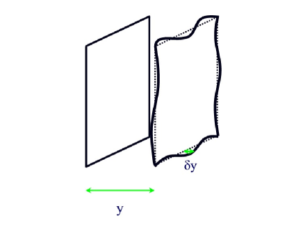
Figure 8: The inflaton field $y$ is interpreted as the distance between the two branes. Quantum fluctuations of this field will give rise upon collision to density perturbations on comoving hypersurfaces. These fluctuations will be later observed as temperature anisotropies in the microwave background.

In fact, the induced metric perturbations in our (3+1)-dimensional universe can be understood as arising from the fact that, due to fluctuations in the approaching D4-branes, inflation does not end at the same time in all points of our 3-dimensional space, see Fig. 8, and the gauge invariant curvature perturbation on comoving hypersurfaces, ${\cal R}_{k}=\delta N_{k}=H\,\delta y_{k}/v$, is non-vanishing, being later responsible for the observed spectrum of temperature anisotropies in the microwave background [33, 34, 35].

7 Reheating the Universe after inflation

Reheating is the most difficult part in inflationary model building since we don’t know to what the inflaton couples to. Eventually one hopes the vacuum energy during inflation will go into relativistic degrees of freedom and everything will finally thermalise so that the hot Big Bang follows. One thing we know for sure is that the universe must have reheated before primordial nucleosynthesis ($T_{\rm rh}>1$ MeV), otherwise the light element abundances would be in conflict with observations. However, since the scale of inflation is not yet determined observationally, we are allowed to consider reheating the universe just above an MeV.

We will briefly describe reheating after brane inflation. The details have not been worked out yet, but we can give here a succint account of what should be expected. Brane inflation ends like hybrid inflation, still in the slow-roll regime, when the string-tachyon becomes massless and the tachyon condenses at the true minimum. In Ref. [37] it was shown that this typically occurs very fast, within a time scale of order the inverse curvature of the tachyon potential, $t_{*}\sim m_{T}^{-1}\equiv(\theta/2\pi\alpha^{\prime})^{-1/2}$. From the point of view of the low energy effective field theory description, this is seen as the decay rate (per unit time and unit volume) or the imaginary part of the one-loop energy density (46).

Figure 9: Splitting of the mass spectrum of the ${\cal N}=4$ Yang-Mills supermultiplet when the angles are non-vanishing or, in the T-dual picture, degenerancy splitting for the first Landau level. $\psi^{\pm}$ are the chiral fermions and $\phi$ are the scalars.

Let us calculate the low energy degrees of freedom in the brane after the collision. This can be extracted from the partition function (13),written here in terms of infinite products,

$$Z(\theta,t) = {(z-1)^{4}\over z}\,\Big{(}\sum_{n=0}^{\infty}z^{2n}\Big{)}\,\prod_{m=1}^{\infty}{(1-q^{m}z)^{4}(1-q^{m}z^{-1})^{4}\over(1-q^{m})^{6}(1-q^{m}z^{2})(1-q^{m}z^{-2})}\,,$$ (43)

$$q = e^{-2\pi t}\,,\hskip 28.45274ptz=e^{-\theta t}\,.$$ (44)

The first factor, $(1-z)^{4}/z=z^{-1}-4+6z-4z^{2}+z^{3}$, gives precisely the lowest lying ${\cal N}=4$ supermultiplet, including the tachyon, see Table 1 and Fig. 9, with the correct multiplicity and (bosonic/fermionic) sign. The fact that $\sum_{i}(-1)^{F_{i}}\,m_{i}^{2n}=0,\ (n=1,2,3)$, ensures that (9) is finite, as it should be, since supersymmetry is only broken spontaneously by the angle $\theta$.

Field	$2\pi\alpha^{\prime}m^{2}$
1 scalar	$y^{2}/(2\pi\alpha^{\prime})+3\theta$
2 massive fermions	$y^{2}/(2\pi\alpha^{\prime})+2\theta$
3 scalars	$y^{2}/(2\pi\alpha^{\prime})+\theta$
1 massive gauge field	$y^{2}/(2\pi\alpha^{\prime})+\theta$
2 massive fermions (massless for $y=0$)	$y^{2}/(2\pi\alpha^{\prime})$
1 scalar (tachyonic for $y=0$)	$y^{2}/(2\pi\alpha^{\prime})-\theta$

Table 1: The mass spectrum of the ${\cal N}=4$ supermultiplet. Notice that the first scalar will be tachyonic if the distance between the two branes is smaller than $y_{c}^{2}=2\pi\alpha^{\prime}\theta$, i.e. the two-brane system becomes unstable.

The next factor in (43) is the sum $\sum_{n=0}^{\infty}z^{2n}=1+z^{2}+z^{4}+z^{6}+\dots$, which corresponds to the Landau levels induced, in the dual picture, by the supersymmetry breaking flux associated to the angle $\theta$. They give, at any order $N$, a supermultiplet with $\sum_{i}(-1)^{F}\,m_{i}^{2n}=0,\ (n=1,2,3)$, so they still provide a finite one-loop potential (9). For a given supersymmetry-breaking angle $\theta$, one should include in the low energy effective theory the whole tower of Landau levels up to $N=1/\theta$.

Finally, one could include also the first low-lying string states, whose masses are determined by the expansion of the infinite products in (43),

$$Z(\theta,t)={(z-1)^{4}\over z}\,\Big{(}\sum_{n=0}^{\infty}z^{2n}\Big{)}\,\Big{[}1+{(1-z)^{4}\over z^{2}}\,q^{2}+{(1-z)^{4}(1+7z^{2}+z^{4})\over z^{4}}\,q^{4}+\dots\Big{]}\,.$$ (45)

Their structure still comes in ${\cal N}=4$ supermultiplets, so they again give a finite Coleman-Weinberg potential.

We will use the whole tower of Landau levels in the effective field theory to connect the one-loop potential at short distances, with the full string theory one-loop potential coming from exchanges of the massless string modes at large distances, responsible for inflation. This connection will be essential for the latter stage of preheating and reheating, because it will provide the low energy effective masses, and the couplings between the inflaton field $y$ and the effective fields living on the D4-brane.

The potential (10) is finite if there are no massless or tachyonic fields. When the tachyon appears, i.e. at distances smaller tham $y_{c}$, there is an exponentially divergent amplitude for $m_{i}=0$. A possible strategy to attach physical meaning to this divergence is to analytically continue the potential (11) in the complex $y$-plane. After the continuation, there is a logarithmic branch point at $y=y_{c}$. In this way, we get rid of the divergence and the potential develops a non-vanishing imaginary part for $y<y_{c}$, which signals the instability of the vacuum.

Figure 10: The attractive inflaton potential between two D4-branes. The red line corresponds to the string-derived potential (11); in blue is the Real part of the Coleman-Weinberg field-theory limit of the same potential (10), and in green is the Imaginary part, which is non-zero only when the tachyon condenses, at $y^{2}<2\pi\alpha^{\prime}\theta$. We have chosen here $\theta=\pi/12$. The potential $V(y)$ and the distance $y$ are both in units of $\alpha^{\prime}=1$.

We have plotted in Fig. 10 the attractive potential $V(y)$ between two D4-branes at an angle $\theta=\pi/12$. The large distance behaviour $y^{2}\gg\alpha^{\prime}$ is determined from the supergravity amplitude (11), in red, while the short distance potential is obtained from the Coleman-Weinberg potential corresponding to the lowest-lying effective fields, which fall into ${\cal N}=4$ supermultiplets. The real part of the Coleman-Weinberg potential is drawn in blue in Fig. 10, while the imaginary part is in green.

In the field theory limit ($q\to 0$ and $z\neq 0$) we can consider the infinite tower of Landau levels, while ignoring the string levels, i.e. $Z(\theta,t)=(z-1)^{4}\,\sum_{n=0}^{\infty}z^{2n-1}$. The finite low energy effective potential at zero separation $y=0$ becomes [1]

$$V(0,\theta)={i\pi-1.70638\over 32\pi^{2}}\,\left({\theta\over 2\pi\alpha^{\prime}}\right)^{2}\,.$$ (46)

The imaginary part can be related, through the optical theorem, with the rate of decay of the false vacuum towards the minimum of the tachyon potential,

$$\Gamma_{\phi}=(2\pi R)^{3}\,{\rm Im}\,V_{\rm 1-loop}\simeq 3\times 10^{-5}\,M_{s}\simeq 2.7\times 10^{8}\ {\rm GeV}\,.$$ (47)

This implies a (perturbative) reheating temperature

$$T_{\rm rh}\simeq 0.1\,\sqrt{\Gamma_{\phi}\,M_{p}}\simeq 3\times 10^{12}\ {\rm GeV}\,,$$ (48)

which coincides with the reheating temperature that would have resulted if all the false vacuum energy would have been converted into radiation soon after symmetry breaking. Note that since the rate of expansion during inflation $H=M^{2}/\sqrt{3}M_{\rm P}$ is much smaller than the mass scale $m_{T}$, the false vacuum energy density $E_{0}=2T_{p}L=M^{4}$ is not diluted by the expansion before reheating, as typically occurs in chaotic inflation, and all of it is converted into radiation, reheating the universe to a temperature

$$T_{\rm rh}=\Big{(}{30\over\pi^{2}g_{*}}\Big{)}^{1/4}\,M\simeq 1\times 10^{12}\ {\rm GeV}\,,$$ (49)

where we have assumed $g_{*}\sim 10^{3}$ for the number of relativistic degrees of freedom at reheating.

However, the actual process of reheating is probably very complicated and there is always the possibility that some fields may have their occupation numbers increased exponentially due to parametric resonance [38] or tachyonic preheating [37]. Moreover, a significant fraction of the initial potential energy may be released in the form of gravitational waves, which will go both to the bulk and into the brane. One must be sure that the bulk gravitons do not reheat at too high a temperature, because their energy does not redshift inside the large compact dimensions (contrary to our (3+1)-dimensional world, where radiation redshifts with the scale factor like $a^{-4}$), and they could interact again with our (presently cold) brane world and inject energy in the form of gamma rays, in conflict with present bounds from observations of the diffuse gamma ray background [36]. Fortunately, since the fundamental gravitational scale, $M_{\rm P}$, in this model is large enough compared with all the other scales, the coupling of those bulk graviton modes to the brane is suppressed, and thus we do not expect in principle any danger with the diffuse gamma ray background [36], but a detailed study remains to be done.

8 Conclusions

We have shown how string theory provides an interesting realization of hybrid inflation, in the context of D-branes wrapped around the compactification scale, where the inflaton is the interbrane separation. The small parameter needed for sufficient inflation and a small amplitude of fluctuations in the CMB is due here to the spontaneous breaking of supersymmetry via a small angle between the branes, which induces a very flat potential for the inflaton.

This model gives a geometrical realization of inflation which is very robust with respect to initial conditions in the compact space. Moreover, the slow-roll conditions can be interpreted as (geometrical) conditions on the relative velocity and acceleration of the branes towards eachother. The number of $e$-folds is directly related to the distance between branes, and metric perturbations, that later give rise to temperature anisotropies, are nothing but fluctuations on the interbrane distance.

The model makes very specific predictions: For a concrete compactification radius in units of the string scale, $2\pi R=60\,l_{s}$, we find a mass scale $M\sim M_{s}\sim 10^{13}$ GeV. Moreover, the radius of compactification turns out to be $R^{-1}\sim 10^{12}$ GeV. The scalar tilt is $n_{s}=0.974$, with negligible scale dependence, $dn_{s}/d\ln k=-3\times 10^{-4}$, and there is an insignificant amount of tensor modes or gravitational waves.

The reheating of the universe occurs through the conversion of all the false vacuum energy during inflation into radiation, as the tachyon condenses and is driven towards its vev. A detailed account of this process is still lacking.

References

- [1] J. García-Bellido, R. Rabadán and F. Zamora, JHEP 0201, 036 (2002) [hep-th/0112147].
- [2] A. D. Linde, Particle Physics and Inflationary Cosmology, Harwood Academic Press (1990); A. R. Liddle and D. H. Lyth, Cosmological inflation and large-scale structure, Cambridge University Press (2000).
- [3] D. H. Lyth and A. Riotto, Phys. Rept. 314, 1 (1999) [hep-ph/9807278].
- [4] A. D. Linde, Phys. Lett. B259, 38 (1991); Phys. Rev. D 49, 748 (1994) [astro-ph/9307002]; E. J. Copeland, A. R. Liddle, D. H. Lyth, E. D. Stewart and D. Wands, Phys. Rev. D 49, 6410 (1994) [astro-ph/9401011]; J. Garcia-Bellido, A. D. Linde and D. Wands, Phys. Rev. D 54, 6040 (1996) [astro-ph/9605094].
- [5] J. Polchinski, String theory. Vols. 1 and 2: Superstring theory and beyond, Cambridge University Press, Cambridge, UK (1998).
- [6] G. Dvali, S.-H. H. Tye, Phys. Lett. B 450, 72 (1999) [hep-ph/9812483].
- [7] G. Dvali, Q. Shafi and S. Solganik, D-brane Inflation, [hep-th/0105203].
- [8] C. P. Burgess, M. Majumdar, D. Nolte, F. Quevedo, G. Rajesh and R.-J. Zhang, JHEP 0107, 047 (2001) [hep-th/0105204].
- [9] C. Herdeiro, S. Hirano and R. Kallosh, JHEP 0112, 027 (2001) [hep-th/0110271].
- [10] K. Dasgupta, C. Herdeiro, S. Hirano and R. Kallosh, Phys. Rev. D 65, 126002 (2002) [hep-th/0203019].
- [11] R. Kallosh, A. D. Linde, S. Prokushkin and M. Shmakova, Phys. Rev. D 65, 105016 (2002) [hep-th/0110089].
- [12] B.-S. Kyae and Q. Shafi, Phys. Lett. B 526, 379 (2002) [hep-ph/0111101].
- [13] G. Shiu and S.-H. Henry Tye, Phys. Lett. B 516, 421 (2001) [hep-th/0106274].
- [14] M. Berkooz, M. R. Douglas and R. G. Leigh, Nucl. Phys. B 480, 265 (1996) [hep-th/9606139].
-
[15]
H. Arfaei, M. M. Sheikh-Jabbari,
Phys. Lett. B 394, 288 (1997) [hep-th/9608167].
M.M. Sheikh-Jabbari, Phys. Lett. B 420, 279 (1998) [hep-th/9710121].
R. Blumenhagen, L. Goerlich and B. Kors, Nucl. Phys. B 569, 209 (2000) [hep-th/9908130].
HEP 0001, 040 (2000) [hep-th/9912204].
S. Forste, G. Honecker and R. Schreyer, Nucl. Phys. B 593, 127 (2001) [hep-th/0008250]. - [16] C. Bachas, A way to break supersymmetry, [hep-th/9503030].
- [17] N. Jones, H. Stoica and S. H. Tye, JHEP 0207, 051 (2002) [hep-th/0203163].
- [18] M. Gomez-Reino and I. Zavala, JHEP 0209, 020 (2002) [hep-th/0207278].
- [19] C. P. Burgess, P. Martineau, F. Quevedo, G. Rajesh and R. J. Zhang, JHEP 0203, 052 (2002) [hep-th/0111025].
- [20] R. Blumenhagen, B. Kors, D. Lust and T. Ott, Nucl. Phys. B 641, 235 (2002) [hep-th/0202124].
- [21] S. Kachru, R. Kallosh, A. Linde and S. P. Trivedi, hep-th/0301240.
- [22] For a review, see F. Quevedo, Class. Quant. Grav. 19, 5721 (2002) [hep-th/0210292].
- [23] T. Banks and L. Susskind, Brane - Anti-Brane Forces, [hep-th/9511194].
- [24] J. Polchinski, Y. Cai, Nucl. Phys. B296, 91 (1988).
- [25] W. Fischler and L. Susskind, Phys. Lett. B 171, 383 (1986); Phys. Lett. B 173, 262 (1986).
- [26] E. Dudas and J. Mourad, Phys. Lett. B 486, 172 (2000) [hep-th/0004165].
- [27] R. Blumenhagen and A. Font, Nucl. Phys. B 599, 241 (2001) [hep-th/0011269].
- [28] A. Sen, Non-BPS states and Branes in string theory, [hep-th/9904207].
- [29] M. R. Douglas, Class. Quant. Grav. 17, 1057 (2000) [hep-th/9910170].
- [30] R. Rabadan, Nucl. Phys. B 620, 152 (2002) [hep-th/0107036].
- [31] J. Garcia-Bellido and R. Rabadan, JHEP 0205, 042 (2002) [hep-th/0203247].
- [32] J. García-Bellido, Astrophysics and Cosmology, European School of High-Energy Physics (ESHEP 99), CERN report 2000-007, p. 109-186 [hep-ph/0004188].
- [33] G. F. Smoot et al. [COBE Collaboration], Astrophys. J. 396, L1 (1992); C. L. Bennett et al. [COBE Collaboration], Astrophys. J. 464, L1 (1996) [astro-ph/9601067].
- [34] C. B. Netterfield et al. [Boomerang Collaboration], Astrophys. J. 571, 604 (2002) [astro-ph/0104460].
- [35] H. V. Peiris et al. (WMAP Collaboration), “First year Wilkinson Microwave Anisotropy Probe (WMAP) observations: Implications for inflation,” astro-ph/0302225.
- [36] N. Arkani-Hamed, S. Dimopoulos and G. R. Dvali, Phys. Rev. D 59, 086004 (1999) [hep-ph/9807344].
- [37] G. N. Felder, J. García-Bellido, P. B. Greene, L. Kofman, A. D. Linde and I. I. Tkachev, Phys. Rev. Lett. 87, 011601 (2001) [hep-ph/0012142]; G. N. Felder, L. Kofman and A. D. Linde, Phys. Rev. D 64, 123517 (2001) [hep-th/0106179].
- [38] L. Kofman, A. D. Linde and A. A. Starobinsky, Phys. Rev. Lett. 73, 3195 (1994) [hep-th/9405187]; Phys. Rev. D 56, 3258 (1997) [hep-ph/9704452].