The Response of Model and Astrophysical Thermonuclear Flames to Curvature and Stretch

Abstract

Critically understanding the ‘standard candle’-like behavior of Type Ia supernovae requires understanding their explosion mechanism. One family of models for Type Ia Supernovae begins with a deflagration in a Carbon-Oxygen white dwarf which greatly accelerates through wrinkling and flame instabilities. While the planar speed and behavior of astrophysically-relevant flames is increasingly well understood, more complex behavior, such as the flame’s response to stretch and curvature, has not been extensively explored in the astrophysical literature; this behavior can greatly enhance or suppress instabilities and local flame-wrinkling, which in turn can increase or decrease the bulk burning rate. In this paper, we explore the effects of curvature on both nuclear flames and simpler model flames to understand the effect of curvature on the flame structure and speed.

1. INTRODUCTION

Type Ia supernovae are used as ‘standard candles’ for cosmology (see the review by Hillebrandt & Niemeyer 2000 and references therein). The standard model for a Type Ia supernova involves a flame that begins deep in the interior of a Carbon-Oxygen Chandrasekhar mass white dwarf, but the full mechanism for explosion is not yet understood. One-dimensional simulations (Woosley et al. 1984; Nomoto et al. 1984) of flame-powered Type Ia can match the energetics of the observations if the flame reaches $\sim$1/3 of the speed of sound as it burns through the star, although the precise mechanism for this flame acceleration is still poorly understood. Other models begin with a flame that accelerates to $\sim$1/30 of the sound speed (Domínguez & Höflich, 2000) and undergoes an as-yet unexplained transition to a detonation (Khokhlov, 1991a, b; Arnett & Livne, 1994a, b). Either mode requires that the flame accelerate considerably beyond its laminar speed, and flame instabilities are generally cited as potential mechanisms. When burning begins, pockets of buoyant, hot ash are formed as the flame propagates outward. This flame is unstable to the Landau-Darrieus and Rayleigh-Taylor instabilities (Bychkov & Liberman, 1995a). These instabilities wrinkle the flame front, increasing the surface area, and therefore, the bulk burning rate.

Both strain from curvature and flow-induced stretch of a flame are known to affect a flame’s speed and structure (Markstein, 1964). These strains change both the local burning rate, and the bulk burning behavior in complex large scale flows (Helenbrook & Law, 1998) through multidimensional flame instabilities. Curvature effects in terrestrial flames have received a great amount of attention (see, for instance, the review by Law & Sung 2000), but the astrophysical flame literature on these effects has been sparse.

The instabilities that might increase the total burning by a flame do so by stretching and curving the flame. Because these strains themselves can significantly change a flame’s local burning rate, the onset and growth rate of flame instabilities are directly affected by curvature. Thus, in the context of the standard Type Ia model, understanding the detailed explosion mechanism requires understanding the micro-physics of the flame propagation in the white dwarf. One way of doing this would be to extend large supernova simulations (eg, Reinecke et al. 2002b, 1999; Niemeyer et al. 1996; Gamezo et al. 2003) to incorporate a fully resolved flame. However, at the onset of the burning, the flame is only $\sim 10^{-5}\ \mathrm{cm}$ thick, inside a star of radius $\sim 10^{8}\ \mathrm{cm}$. At lower densities, the flame becomes broader, but remains tiny compared to the radius of the whole star. Thus any realistic study of multidimensional Type Ia scenarios that follow a significant portion of the star requires understanding of the behavior of the flames, and must use a model on unresolved scales to describe the burning physics, such as flame-stretch interactions and the corresponding effects on instabilities. Some such models exist (Khokhlov, 1995; Reinecke et al., 2002a), but they are based on the properties of large scale flows and terrestrial scalings, rather than on the local physical properties of astrophysical flames. A detailed understanding of the flame’s response to curvature is necessary input to a subgrid scale flame model.

In this paper, we describe numerical experiments of propagating, spherical flames, similar to recent experiments and calculations performed by the chemical combustion community (Bradley et al., 1996; Karpov et al., 1997; Aung et al., 1997; Hassan et al., 1998; Bradley et al., 1998; Sun et al., 1999; Gu et al., 2000), designed to measure the flame structure and speed response to geometric curvature. All of the flame simulations presented are 1-d (either in planar or spherical geometry), to get clean and unambiguous measurements of the flame’s response to curvature. As the flame propagates to different radii, it experiences different strain due to the geometry, parameterized by a dimensionless strain rate, $\mathrm{Ka}$, defined in later sections. Quantitatively, we seek the modified flame velocity

$$S_{l}=S_{l}^{0}\cdot f(\mathrm{Ka}),$$ (1)

where $S_{l}$ is the laminar flame speed, and $S_{l}^{0}$ is the uncurved laminar flame speed. (Throughout this paper, a superscript 0 will refer to planar, unstretched flame quantities.)

Markstein (1964) postulated a flame-speed law of the above form for small curvatures based on empirical results. Expressed in dimensionless numbers, this is written:

$$S_{l}=S_{l}^{0}\cdot\left(1+\mathrm{Ma}\,\mathrm{Ka}\right),$$ (2)

where $\mathrm{Ma}$ is the dimensionless Markstein number, which depends on parameters of the flame. We refer to this as the Markstein relation. The Markstein number can be negative or positive for any given flame. A negative Markstein number indicates that the flame would burn more slowly in regions of positive curvature ($\mathrm{Ka}>0$) and more quickly in regions of negative curvature ($\mathrm{Ka}<0$), and the reverse is true for a flame with positive Markstein number.

The Markstein relation has proven very robust for describing flame behavior in terrestrial flames. In that context, work has been done to calculate Markstein numbers from first principles (for example, Clavin & Williams 1982; Matalon & Matkowsky 1982; Chung & Law 1988) and from numerical or physical experiments (for example, Karpov et al. 1997; Müller et al. 1997; Kwon & Faeth 2001; Aung et al. 1998; Gu et al. 2000; Hassan et al. 1998; Bradley et al. 1996, 1998; Sun et al. 1999). In this paper, we discuss its applicability to astrophysical thermonuclear flames and examine the flame-curvature relation both for these flames and for simpler model flames with parameters that may be varied to understand their effects.

We outline some theory relevant to our study in §2. In §3 we discuss the methods used in the numerical experiments. These experiments, which are described in §4, were performed to understand how the flame speed changes with curvature. In §5 we present the results of these experiments, and we conclude in §6. The appendix provides some simple tests that provide verification of our code for the present simulations.

2. THEORY

2.1. Planar Astrophysical Flame Structure

The structure of an astrophysical flame is sketched in Fig. 1. Between the unburned state (which throughout this paper we will label with a subscript $u$) and the burned state (subscript $b$), there are two distinct regions. There is a ‘preheat’ zone, where energy from the reactions and the already-hot ash diffuses outwards and heats the incoming (in the frame of the flame) fuel, and there is a reaction zone where the bulk of the thermonuclear reactions occur. The interface between these two zones — the state at which burning begins — we will denote with subscript $i$. Because the flame moves very slowly compared to the sound speed in the domain (Timmes & Woosley, 1992), the pressure is nearly constant throughout the unburned fuel and burned ash, $P_{b}\approx P_{u}=P$. It is possible, however, for the pressure to differ significantly from this value in the flame structure itself, because of the exothermic reactions taking place there.

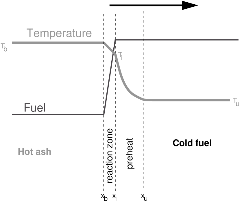
Figure 1.— A schematic of an astrophysical thermonuclear flame, propagating to the right. The exothermic reactions are largely concentrated in a very thin reaction zone, and energy from that region diffuses into the cold fuel over a large preheat zone.

The astrophysical flames of interest to us here are ‘pre-mixed’ — that is, the combustible fuel is waiting only for sufficient heat to ignite. Thus, the speed of propagation of the flame is determined completely by two rates — the rate of energy input by the reaction, and the rate at which enough heat is diffused outwards to ignite the as-yet unburned fuel.

Astrophysical premixed flames differ from their terrestrial counterparts in several respects. If we were to sketch a terrestrial flame in Fig. 1, we would have, overlapping with the thermal diffusion zone, a material diffusion zone where fuel diffuses inwards towards the fuel-depleted burned zone. The Lewis number, $\mathrm{Le}$, describes the relative importance of thermal and species transport across a flame; in terms of the thermal diffusivity $D_{th}$ and the material diffusivity $D_{s}$, $\mathrm{Le}=D_{th}/D_{s}$. In the astrophysical flames we consider here, the Lewis number is of order $10^{7}$ (Timmes & Woosley, 1992), whereas in terrestrial flames, the Lewis number is often of order unity. Since for astrophysical flames, the effect of species diffusion is insignificant compared with thermal diffusion, we neglect species diffusion for astrophysical and some model flames; in those cases, we informally speak of an infinite Lewis number. Note, however, that in these numerical simulations, numerical diffusion will result in some small species diffusion.

Astrophysical flames also have extremely peaked energy-generation rates — that is, rates which are strongly dependent on temperature. This is usually described by a Zeldovich number, $\mathrm{Ze}$, defined as

$$\mathrm{Ze}=\frac{T_{a}}{T_{b}}\frac{T_{b}-T_{u}}{T_{b}}\enskip.$$ (3)

Here, $T_{a}$ is an activation temperature that sets the burning rate by representing an activation energy for the reaction, such as a potential energy barrier that must be overcome for the reaction to proceed, and $T_{b}$ and $T_{u}$ are the temperatures of the burned and unburned gas. In hydrocarbon-air burning, this number is typically of order 10 (Glassman, 1996); most of the flames we will see here will have similar ratios, meaning similarly peaked energy generation rates.

Astrophysical flames also typically occur in electron-degenerate material, meaning that the large amounts of energy input to the flow (much larger compared to the ambient energy density than in terrestrial flames) result in comparatively small density changes at the roughly constant pressure relevant for flame problems. The ratio of the burned-gas density to the unburned-gas density will be parameterized by $\alpha=\rho_{u}/\rho_{b}$. Another factor contributing to a relatively low $\alpha$ in astrophysical flames is that these flames are powered by fusion, so that the mean molecular weight of the ash behind the flame is, unlike many chemical flames, greater than the mean molecular weight of the fuel ahead of it.

The reactions are governed by a strongly-peaked burning rate (ie., large $\mathrm{Ze}$), so that in the preheat zone, the fuel can get quite hot without any significant burning taking place; instead all of the burning occurs only in the hottest region, in a narrow burning zone. In this case, a method for estimating the flame velocity which dates back to Zeldovich & Frank-Kamenetskii (1938) shows the most important physical effects. For a planar, steady flame, one can consider the energy equation in the reference frame of the flame front itself, and match boundary conditions between the non-burning preheat zone where thermal conductivity is important, and a narrow reaction zone. If one uses a canonical peaked temperature dependence for a burning rate used in combustion theory, an Arrhenius law (see, for example, textbooks such as Zeldovich et al. (1985); Glassman (1996); Williams (1985)), which is exponential in the ratio $-T_{a}/T$, and consider our nuclear generation rate to be from a second-order (eg., ${\mathrm{fuel}}+{\mathrm{fuel}}\rightarrow{\mathrm{products}}$, so that the reaction depends on the square of the fuel concentration) then the reaction rate is

$$\dot{\epsilon}_{\mathrm{nuc}}=a\rho X_{f}^{2}e^{-T_{a}/T},$$ (4)

where $X_{f}$ is the fuel mass fraction, then one can find

$$S_{l}^{0}=\sqrt{2\frac{\sigma_{b}}{(C_{p})_{b}^{2}}\frac{a{X_{f}}_{u}^{2}}{T_{a}}e^{-T_{a}/T_{b}}}.$$ (5)

where $\sigma$ is the thermal conductivity and $C_{p}$ is the specific heat at constant pressure.

This approach is sufficient to get velocities for the astrophysical flames we describe here to within a factor of a few, and demonstrates the most important physical effects. A more careful analysis by Bychkov & Liberman (1995b), using asymptotics and explicitly including an equation of state and conductivity suitable for completely degenerate materials, can model the laminar flame speeds to within 25–50%.

2.2. Wrinkling

Above, we have assumed a planar flame. Now consider Fig. 2. In curved regions of the flame, heat transport into the cold fuel can be concentrated or diluted by simple geometry of the wrinkling, affecting the flame speed and structure in those regions. Since astrophysical flames propagate by thermal conduction, when the heat transport is concentrated by negative curvature, we would expect the flame to propagate faster, and when heat transport is diluted by positive curvature, we would expect the flame to propagate more slowly.

Figure 2.— A schematic of a wrinkled flame, with the direction of propagation shown by the large arrow. Heat diffuses from the burning zone to the cool fuel as shown by the little arrows across the flame. At regions of positive (negative) curvature, heat diffusion is ‘diluted’ (concentrated), and flame propagation will slow down (speed up).

Note that this figure does not describe cusping of an interface moving at constant velocity, such as in the Landau-Darrieus instability. Here, we emphasize that the flame speed itself will change along the flame; if the flame speed were to vary strongly enough, cusping need not occur.

The change in geometry can be taken into account by including area terms into the equations of the previous section, and we can derive results that include geometric effects due to curvature. This was done, for instance, in Law & Sung (2000). Defining the strain due to the curvature with a dimensionless Karlovitz number,

$$\mathrm{Ka}_{C}=\frac{dA}{A}=\frac{A(x_{u})-A(x_{b})}{A(x_{u})}\approx l_{f}\frac{1}{A}\frac{dA}{dx},$$ (6)

where $x_{b}$ and $x_{u}$ are the position of the burned and unburned material, respectively, and $l_{f}$ is the thickness of the flame. We then find to linear order in $\mathrm{Ka}_{C}$,

$$S_{l}=S_{l}^{0}\left(1+\left(\frac{1}{\mathrm{Le}}-1\right)\frac{\mathrm{Ze}}{2}\mathrm{Ka}_{C}\right),$$ (7)

and so for our large-Lewis number flames,

$$S_{l}=S_{l}^{0}\left(1-\frac{\mathrm{Ze}}{2}\mathrm{Ka}_{C}\right).$$ (8)

Note that the Karlovitz number is defined so that it is negative if the area at the burned fluid is greater than that at the unburned fluid, ie. for regions of negative curvature. Thus, since $\mathrm{Ze}>0$, we get flame speed enhancement in negatively curved regions, which is as we expect. Also notice that the effect is strongest for flames with very peaked temperature dependencies, where the geometrically-induced difference in temperature diffusion will have a large effect.

2.3. Stretch due to flow

A steady spherical flame will feel the strain described above. Another contribution to strain in the flame comes from the flow — for instance, a flame propagating outward will also be advected outward by the expansion of material behind it. Any such flow will also lead to a strain, characterized by a strain rate $K=(1/A)(dA/dt)$ where $A$ is the area of the flame surface. For the spherical flames we consider here, $A=4\pi r^{2}$, so that

$$K=\frac{2}{r_{f}}u_{\mathrm{gas}},$$ (9)

where $r_{f}$ is the radius of the flame’s position, and $u_{\mathrm{gas}}$ is the flow velocity of the gas at the flame’s location. This strain can be converted to a dimensionless Karlovitz number by considering the strain over a flame crossing time, $l_{f}/S_{l}^{0}$:

$$\mathrm{Ka}_{S}=\frac{2l_{f}}{r}\frac{u_{\mathrm{gas}}}{S_{l}^{0}}.$$ (10)

Note that for a flame in a medium where the flow is zero, this strain vanishes.

One can also consider a total strain rate, $\mathrm{Ka}_{T}=\mathrm{Ka}_{C}+\mathrm{Ka}_{S}$. We can meaningfully do this for the purposes of assessing the effect on flame velocity; Groot et al. (2002) demonstrated that a single Markstein number can be found that is meaningful for the combined effects of stretch and curvature, and in fact considering only the stretch is problematic. We note here that other works in the literature choose different sign conventions for $\mathrm{Ka}$ and $\mathrm{Ma}$.

2.4. Effect on Landau-Darrieus growth rate

The change in flame speed as a function of curvature can modify multidimensional flame instabilities. The Landau-Darrieus instability (Landau & Lifshitz, 1987) is often proposed as a mechanism for accelerating the burning rate of a flame in a white dwarf. In an otherwise planar flame with a density ratio $\alpha=\rho_{u}/\rho_{b}$, a sinusoidal ‘wrinkle’ of wavenumber $k$ will grow in the linear regime with an exponential growth rate

$$\omega=\frac{\alpha kS_{l}^{0}}{\alpha+1}\left(\sqrt{\frac{\alpha^{2}+\alpha-1}{\alpha}}-1\right).$$ (11)

One can re-derive the linear theory of Landau-Darrieus growth rates with the non-constant flame speed given in Equation 2 and arrive at (Zeldovich et al., 1985)

$$\omega=\frac{\alpha kS_{l}^{0}}{\alpha+1}\left(\sqrt{\frac{\alpha^{2}+\alpha-1}{\alpha}+kl_{f}\mathrm{Ma}(kl_{f}\mathrm{Ma}+2\alpha)}-1+kl_{f}\mathrm{Ma}\right),$$ (12)

where $l_{f}$ is the thermal width of the flame. In fact, some authors (for example, Clanet & Searby (1998)) have used this to measure the Markstein number of a flame from an experimentally determined growth rate of the instability.

From our discussion of the effects of positive and negative Markstein number, we expect our astrophysical flames to have $\mathrm{Ma}<0$. In this case, the Landau-Darrieus growth rate is reduced, and indeed modes $k>(\alpha-1)/(2\alpha l_{f}|\mathrm{Ma}|)$ are stable against the Landau-Darrieus instability. In a negative Markstein number flame, the flame-curvature relation works against a wrinkle trying to increase in size; the ‘peaks’ of the flame burn more slowly, because they’re at positive curvature, so they tend to fall back, and the ‘troughs’ of the flame at negative curvature burn faster and catch back up.

For linear perturbations, the increased burning rate caused by a linear curvature term at ‘troughs’ in the wrinkle is exactly offset by a decreased burning rate at the ‘peaks’, so that the total burning rate remains proportional to the surface area of the flame, as in the constant flame velocity case. Thus the total burning rate is decreased by the decreased growth rate of the instability. If cusping occurs when the perturbation becomes nonlinear, then (fast-burning) regions of negative curvature decrease to almost zero in favor of regions of (slow-burning) positive curvature, which further decreases the net burning rate.

Thus, for understanding the behavior of the Landau-Darrieus instability in astrophysical phenomenon, at least the curvature behavior of the flame must be modeled. An alternative is to model the entire flame behavior, as in Bychkov & Liberman (1995a), where a careful analysis of the linear growth rate and linear instability of a degenerate thermonuclear flame to the Landau-Darrieus instability was performed. These authors also find a cut-off beyond which modes are stable. Another work, Niemeyer & Hillebrandt (1995), studied the instability numerically, although that work obtained anomalous results. In both analytic cases, there is a most-unstable mode; there is some evidence (Helenbrook & Law, 1998) that it is this mode which grows fastest in a flame going through a complex or turbulent flow field if there is power on this scale, and indeed there are other suggestions (Denet, 1998) that small scale wrinkling can directly induce larger-scale wrinkling.

3. NUMERICAL METHODS

We consider two classes of flames — ‘model’ flames and ‘astrophysical’ flames. The delineation is reflected in the input physics. In the simpler, ‘model’ case, we use a polynomial or simple exponential expression for the burning and a simple ideal gas equation of state. At the complex, astrophysical end, we use a relativistic, degenerate equation of state (EOS) and a more astrophysically relevant reaction rate. In this section we review the physics used in the astrophysical-flame simulations. Similar details for the model flames are described in Appendix C.

3.1. Hydrodynamics

For the hydrodynamics, we use the PPM (Colella & Woodward, 1984) compressible hydrodynamics module in the Flash code (Fryxell, 2000). PPM is a widely used Godunov method, which solves the Euler equations in conservative form using a finite-volume discretization. Our implementation of PPM is described in depth in Fryxell (2000), and the PPM module in particular has been tested rigorously in Calder (2002). The Riemann solver is capable of dealing with a general equation of state, following the method outlined in Colella & Glaz (1985).

To accurately follow reactive flows, a separate advection equation is solved for each species,

$$\frac{\partial\rho X_{i}}{\partial t}+\nabla\cdot{\rho X_{i}v}=\rho R_{i}\enskip,$$ (13)

where $X_{i}$ is the mass fraction of species $i$, subject to the constraint that they sum to unity, and $R_{i}$ is the net rate of change in the abundance of species $i$ due to the nuclear burning. $\dot{\epsilon}_{\mathrm{nuc}}$ and $R_{i}$ are related by

$$\dot{\epsilon}_{\mathrm{nuc}}=\sum_{i}{\epsilon_{bi}R_{i}}\enskip,$$ (14)

where $\epsilon_{bi}$ is the binding energy per mass of species $i$.

3.2. Equation Of State

Astrophysical flames in degenerate white dwarf material have a complicated equation of state. Contributions from the ions, electrons, and radiation must be accounted for. The ions are assumed to be fully ionized, and we use an ideal gas expression for them, as described above. Finally, the radiation term is simply blackbody. Full details of the implementation of this EOS can be found in Timmes & Swesty (2000).

The equation of state is responsible for much of the character of astrophysical flames. For the conditions that we consider, the pressure is dominated by the degenerate electron contribution. The degeneracy means that pressure responds only weakly to temperature changes, so the resulting density jumps behind the flame are smaller than they would be with a pure ideal gas EOS (and everything else kept the same).

3.3. Diffusion

Diffusion is implemented in Flash with explicit time differencing in an operator-split manner. The heat flux term is added to the energy evolution equation

$$\frac{\partial\rho E}{\partial t}+\nabla\cdot\left(\rho E+P\right){\bf v}=\nabla\cdot(\sigma\nabla T)+\rho\dot{\epsilon}_{\mathrm{nuc}}{(X_{i},\rho,T)}.\enskip$$ (15)

Here, $E$ is the total energy per unit mass, $P$ is the pressure, ${\bf v}$ is the velocity, $T$ is the temperature, $\sigma$ is the conductivity, $\dot{\epsilon}_{\mathrm{nuc}}$ is the energy source term from burning, $X_{i}$ is the mass fraction of species $i$, and $\rho$ is the total density. The heat flux $-\sigma\nabla T$ is computed during the hydrodynamic step and added to the total energy flux computed by the PPM solver. The fluxes are then used to update the energy in each zone. This implementation preserves the conservative nature of the algorithm.

Because the diffusion is calculated explicitly, the diffusion term adds an additional timestep constraint

$$dt\leq\frac{1}{2}\frac{\delta x^{2}}{D_{th}},$$ (16)

where $D_{th}$ is the diffusion coefficient, $D_{th}={\sigma}/({\rho C_{P}})$. The simulation evolves at either the diffusion timestep or the CFL timestep — whichever is smaller.

For our more realistic thermonuclear flames, the thermal diffusion is the only diffusive process modelled. For some of our model flames, we allow finite $\mathrm{Le}$, and so species diffusion is also calculated; the computation proceeds in the same manner. This is described in Appendix C.

Since these diffusion modules were not included in the original Flash code paper (Fryxell, 2000), we include in Appendix A tests of the correctness of the diffusion operators in Cartesian and spherical coordinates.

3.4. Conductivity

For testing purposes and for our model flame propagation problems in Appendix C, we use a simple constant diffusivity to describe the heat transfer. However, the conductivity for astrophysical flames of interest to the Type Ia problem is much more complicated. For degenerate carbon, electron-electron and electron-ion collisions are important processes in heat transport. The conductivity in the post-flame state can be some 3 orders of magnitude higher than that of the pre-flame state, making a constant conductivity a bad approximation. We use a stellar conductivity routine that includes these processes as well as radiative opacities (Timmes, 2000).

3.5. Burning

We experiment with several reaction rates and networks for our flame simulations. In this paper, we use one-step irreversible reactions, with increasingly complex reaction rates. In all cases the energy release from the nuclear burning is computed in an operator split fashion. After the hydrodynamics are evolved, the reaction network computes the energy release and change in nuclear abundances over the course of the hydro timestep. This energy release is then added to the internal energy of that zone, and a new temperature is computed. For these fully-resolved flames, the CFL-limited timestep from the explicit hydrodynamics is much smaller than the timescale to significantly change the temperature by burning, so that explicit coupling is not needed. We describe the burning rates for our astrophysical flames here; model flame burning is described in Appendix C.

3.5.1 One-step Carbon Burning

The astrophysically-motivated reaction we use is a one-step ¹²C + ¹²C reaction. The rate comes from Caughlan & Fowler (1988) (we refer to this as the CF88 reaction network) and converts two ¹²C nuclei into a single ²⁴Mg nuclei, releasing $5.57\times 10^{17}\mathrm{erg}\ \mathrm{g}^{-1}$. Following the notation of Caughlan & Fowler (1988), the reaction rate is

$$\frac{\mathrm{d}X_{C}}{\mathrm{d}t}=-\frac{1}{12}X_{C}^{2}\rho N_{A}\lambda,$$ (17)

where

$$N_{A}\lambda=4.27\times 10^{26}\frac{T_{9,a}^{5/6}}{T_{9}^{3/2}}\exp\left\{{\frac{-84.165}{T_{9,a}^{1/3}}-2.12\times 10^{-3}T_{9}^{3}}\right\},$$ (18)

where $T_{9}=T/10^{9}\ \mathrm{K}$, $T_{9,a}={T_{9}}/{1.0+0.0396T_{9}}$, and $X_{C}$ is the mass fraction of ¹²C. For each ²⁴Mg nucleus created, 13.933 MeV is released.

This is the main reaction involved in a pure carbon flame in a white dwarf. We treat all other species (eg. ¹⁶O) simply as inert dilutants that serve only to reduce the effective burning rate. We assume here that other reactions (eg. ²⁴Mg($\alpha$,$\gamma$)²⁸Si burning), if modeled, would occur well behind the flame and would not be as important in setting the properties of the flame.

With this reaction mechanism, we neglect any ion screening, for simplicity. Screening is not an important effect except at low temperatures or high densities. At high densities, a one-stage reaction as modeled by this rate might have other problems; late stage reactions could be important. Conversely, low temperatures are not of interest to us for these flame-propagation problems. Thus we restrict ourselves to regimes where screening is unimportant.

3.6. Boundary Conditions

Boundary conditions for subsonic flows in a compressible code are non-trivial. The zero-gradient/outflow condition usually used is insufficient, since not all the characteristics at the edge of the computational domain will be leaving the domain. This means that some information can enter the domain from the boundary and introduce noise into the flame solution.

Boundary conditions for a subsonic outflow have been proposed (see for example Thompson 1987; Hedstrom 1979), but no well-accepted general solutions exist. These boundary conditions try to extend the solution into the boundary conditions in such a way that information is not transmitted into the domain from the boundaries. We choose problem-specific boundary conditions that allow most waves to leave the domain. We first use the fact that, to a good approximation, the pressure is constant in the burned and unburned regions, and since the flames are not in a closed vessel, the pressures will be constant in time. This allows us to set the pressure in the boundary conditions as a constant. Furthermore, since we want heat to diffuse out, the temperature boundary condition is simply set to be zero-gradient. The boundary conditions for the mass fractions are also zero-gradient. This gives us enough information to find a thermodynamically consistent density through our equation of state. Finally, the velocity in the boundary conditions is found by enforcing mass conservation,

$$\rho_{i}v_{i}A_{i}=\rho_{i+1}v_{i+1}A_{i+1}$$ (19)

if the velocities are out of the domain, or zero if the velocities are inwards. Here $A_{i}$ is the area of the face through which the material flows; in planar geometry, this cancels out, but it is important in the spherical geometries we consider. A demonstration that this boundary condition functions in the way we’d like is given in Appendix A.

For our spherical runs, we use at $r=0$ a reflecting boundary condition. This boundary condition is required by the geometry; spherical symmetry requires, for any quantity $f(r)$ other than the radial velocity, $f(r)=f(-r)$, and for the radial velocity, $v_{r}(r)=-v_{r}(-r)$. This is exactly the reflecting boundary condition as implemented in the Flash  code (Fryxell, 2000).

3.7. Adaptive Mesh Refinement

Flash employs an adaptive mesh through the PARAMESH package (MacNeice et al., 2000), allowing it to put computational zones where the resolution is needed and to follow smooth flow with less resolution. The Flash mesh adapts by dividing the domain in half in each dimension, creating new blocks (2 in 1-d, 4 in 2-d, 8 in 3-d) that are logically the same as their parent (typically containing 8 computational zones in each direction) but with twice the spatial resolution. Each new block is checked to see if more refinement is needed, and if so, it is further subdivided. When a block is refined, the newly created children need to be initialized with information from their parent. To obtain higher-order accuracy, a quadratic polynomial is fit to the data of the parent zone and the two zones on either side of it. This procedure is described in detail in Appendix B.

When evolving a flame, it is only necessary to put the resolution near the reaction and diffusion zones. We refine when the second derivatives of density or pressure and are large (the former is expected to be large at the fuel/ash interface, and the latter in the burning region). We also refine on the second derivatives of the nuclear energy generation rate and temperature. The methods for evaluating the derivatives and determining their magnitude is discussed elsewhere (Fryxell, 2000). These criteria ensure that the region around the flame is highly resolved.

4. EXPERIMENTS

4.1. Overview

To numerically investigate the effect of curvature on astrophysical flame speed, we conduct numerical experiments of 1-d model and astrophysical flames running out from, and in toward, the center of a spherical domain, as has been done in the terrestrial combustion community experimentally and computationally (eg., Karpov et al. 1997; Müller et al. 1997; Kwon & Faeth 2001; Aung et al. 1998; Gu et al. 2000; Hassan et al. 1998; Bradley et al. 1996, 1998; Sun et al. 1999). Doing so allows us to examine the flame speed and structure for a range of curvatures and strain rates, both positive and negative, by taking snapshots of the flame at varying positions (and thus curvatures) throughout the domain. We simulate the same flames in planar geometry for comparison.

Focusing on 1-d is computationally more efficient and allows us to separate the pure strain and curvature effects from more complicated multidimensional instabilities, which will be the focus of a later paper. In addition, for the present work, we studied the effects of resolution on the experiments and measurements. The details are discussed in Appendix A.4. In the numerical experiments we present, the flames were sufficiently well-resolved to accurately model the flame structure and speed.

We begin with the simpler model flames, adjusting parameters to ensure we understand the effects of each. For each set of input physics (EOS, reaction mechanism, and model parameters), we simulate three flames — a planar flame, a spherical flame propagating out from the center, and a spherical flame propagating toward the center. We then continue on with simulations of a simplified astrophysical reaction rate with a complex EOS.

In each case, we ignite the flame by placing hot ash — at a temperature corresponding to the ambient planar burned temperature of the flame, unless stated otherwise — alongside the cold fuel we wish to burn, in pressure equilibrium. Neglecting to place the fuel and ash in pressure equilibrium will generate strong pressure waves, especially in non- or partially degenerate fluids, giving spurious results — one is no longer studying a flame, but a transient pressure-driven reaction front. We believe this is the reason for the anomalous results found in Niemeyer & Hillebrandt (1995), which have not been reproduced in work since.

For planar flames, and for the outer boundary conditions for our flames in spherical coordinates, we use the constant-pressure boundary conditions described in §3. For the inner boundary conditions in spherical coordinates, we use reflecting (or ‘symmetry’) boundary conditions at $x=0$ to be consistent with the spherical geometry. These boundary conditions are consistent with those used in the terrestrial combustion literature, eg., (Sun et al., 1999).

4.2. Measuring flame position

One of the most fundamental things we need to do is to measure the flame’s position ($r_{f}$) at different times. Since flames have finite thickness, ‘the’ flame position is ambiguous. Following Groot et al. (2002), we take the flame’s position to be that of the reaction zone, which is less sensitive to strain and curvature effects than, for instance, the outside of the preheat zone. Then a consistent Markstein number can be calculated that includes the effects of curvature and stretch. Since even the reaction zone has finite thickness, we consider several measures for the position of the reaction zone. The first is the most obvious, the position of maximum $\dot{\epsilon}_{\mathrm{nuc}}$. This has the advantage of simplicity, but could potentially be noisy, since extrema are generally not numerically well behaved. Another is $\left<\dot{\epsilon}_{\mathrm{nuc}}x\right>/\left<\dot{\epsilon}_{\mathrm{nuc}}\right>$, an $\dot{\epsilon}_{\mathrm{nuc}}$-weighted position. Since $\dot{\epsilon}_{\mathrm{nuc}}$ is very strongly peaked, this should localize the flame. Clearly, in the limit of a delta-function $\dot{\epsilon}_{\mathrm{nuc}}$, this measure reduces to finding the $x$ of maximum $\dot{\epsilon}_{\mathrm{nuc}}$, but as an integral quantity, it will vary more smoothly. A third measure is where the fuel concentration is most rapidly changing — the location of maximum $dX_{f}/dx$. A fourth is a temperature criterion, the location of maximum $d^{2}T/dx^{2}$. In Fig. 3, we show the results of using these measures for a simulation with a KPP flame and an Arrhenius flame. The KPP flame has a reaction zone approximately $6~{}{\mathrm{cm}}$ wide in a domain of $500~{}{\mathrm{cm}}$, and the Arrhenius flame has a reaction zone of approximately $1/2~{}{\mathrm{cm}}$ in a domain of $100~{}{\mathrm{cm}}$.

Figure 3.— Position versus time, measured four different ways, for both a KPP (left) and an Arrhenius (right) flame. Both flames have $\mathrm{Le}=\infty$ and are propagating spherically outwards. Results from all four position measures are plotted on the top. On the bottom are plotted differences from using $\left<\dot{\epsilon}_{\mathrm{nuc}}x\right>/\left<\dot{\epsilon}_{\mathrm{nuc}}\right>$. The three other methods are: maximum $\dot{\epsilon}_{\mathrm{nuc}}$ (+), maximum $d^{2}T/dx^{2}$, (-), and maximum $dX_{f}/dx$ ($\diamond$). The KPP flame has a reaction zone of $6{\ \mathrm{cm}}$, and the Arrhenius flame has a reaction zone of $1/2{\ \mathrm{cm}}$. The Arrhenius reaction takes about 50 seconds to ignite a self-sustaining flame; before then, any measure of ‘flame position’ is necessarily meaningless.

Because the KPP reaction zone is so wide and includes the preheat zone, finding an unambiguous ‘location’ is especially difficult. The reaction rate depends as strongly on fuel as on temperature, so the fuel-change rate is fastest right at the front of the flame. Also, the energy generation rate is large in a wide region, so averaging over $\dot{\epsilon}_{\mathrm{nuc}}$ produces a position that lags well behind the front of the zone.

For the Arrhenius rate, however, once ignition occurs, all of the direct burning measures ($\dot{\epsilon}_{\mathrm{nuc}}$, $\left<x\dot{\epsilon}_{\mathrm{nuc}}\right>/\left<\dot{\epsilon}_{\mathrm{nuc}}\right>$, and $dX_{f}/dx$) fall almost exactly on top of each other, with only the temperature measure leading slightly, as the temperature must start diffusing outward from the burning region to change the temperature’s second derivative.

In light of the above, we use the $\dot{\epsilon}_{\mathrm{nuc}}$-weighted position as a marker for the position of the reaction zone, and thus the flame, for flames with strongly-peaked reaction networks (Arrhenius, CF88) as it generates fairly clean velocities through differencing and is otherwise essentially degenerate with the very intuitive maximum-of-$\dot{\epsilon}_{\mathrm{nuc}}$ measure of position. For KPP, we use the position of maximum $\dot{\epsilon}_{\mathrm{nuc}}$.

4.3. Measuring flame thickness

The thermal thickness of the flame is an important quantity, setting the length scale for relevant microphysical effects. Since this width is set by a diffusive process, however, its precise start and end are poorly defined. We use two measures of the flame thickness, both used in the literature, that span the range of reasonable measures of the thickness. Both are based on the change in temperature from the burned to unburned state, $\Delta T=T_{b}-T_{u}$.

The first way we use to measure flame thickness, method I, is the ‘10/90’ approach used for instance in Timmes & Woosley (1992). It measures the distance from where the temperature crosses 10% above the unburned temperature to 90% of the way to the burned temperature

$$l_{f}^{(I)}\equiv x(T=T_{b}-.1\Delta T)-x(T=T_{u}+.1\Delta T).$$ (20)

This gives quite wide thermal widths, as it measures well into the diffusive tails of the thermal structure.

The second measure, method II, used for instance in Sun et al. (1999), finds the width by dividing the temperature difference by the maximum temperature gradient in the flame

$$l_{f}^{(II)}\equiv\frac{\Delta T}{\max|\nabla T|}.$$ (21)

This measure gives the thinnest meaningful thermal thickness of the flame, as any smaller thickness must imply a larger thermal gradient than any that exists in the flame structure. We report both flame thicknesses and use them to constrain measurement uncertainties in derived quantities that depend on flame thickness.

4.4. Measuring flame velocity

The velocity we are interested in is not the change of flame position over time ($dr_{f}/dt$), but the rate at which the flame is consuming fuel. This means we want to measure the flame speed with respect to the fuel. The expansion of hot burned ash smoothly generates a velocity field as the flame passes through. In the case of spherical geometry, the velocity of the material between the flame and the origin is zero, since the material has no place to go, and thus the only nonzero velocities are exterior to the flame. In the open planar geometry, material can flow freely through both boundaries. In both cases, the continuity condition requires $A\rho u={\mathrm{const}}$ on either side of the flame. Fig. 4 sketches idealized velocity profiles for the three configurations.

Figure 4.— The gas velocity structure of a propagating flame with the flame propagating outward through a spherical domain (top), through a planar domain (middle), and inward in a spherical domain (bottom). In the closed geometries, the left state, either burned or unburned, has a velocity of zero imposed by the boundary and the continuity condition, $A\rho v={\mathrm{const}}$.

To find the propagation velocity into the fuel, one approach is to find the change in the flame’s position over time (by differencing, or by fitting and then differentiating) and to subtract off the gas velocity (which can be directly measured). This can be problematic, however, especially in the outward-expanding flame case. The expanding gas, especially for large density contrasts, will be a large component of $dr_{f}/dt$, and thus any subtraction is likely to be noisy — especially since the flame velocity and the gas velocity are found in different ways. The situation is worse in the spherical case, as gas velocity has a non-constant spatial structure, adding difficulty to measuring ‘the’ gas velocity.

Another approach, used in the chemical literature (eg., Aung et al. 1997; Hassan et al. 1998), is to note that if the flame is a discontinuity, it must separate two regions with the same momentum flux in the frame of the flame. Given that in the lab frame, the velocity interior to the flame is zero, the flame propagation velocity must be $(\rho_{b}/\rho_{u})(dr_{f}/dt)$. However, this is an approximation that assumes an infinitely thin flame, and we are measuring effects explicitly due to the finite structure of the flame. A better approximation, $(A_{b}\rho_{b})/(A_{u}\rho_{u})(dr_{f}/dt)$, includes the effects of geometry but requires locating ‘the’ position of the unburned and burned states, adding uncertainty due to the ambiguity of those locations.

Since what we are really interested in is the burning rate, which is directly measurable, another approach is simply to measure the total burning rate, $\dot{E}=\int\dot{\epsilon}_{\mathrm{nuc}}\rho dV$. If one then assumes that the reaction region is thin (a better approximation than assuming the thermal structure of the flame to be thin), then one can compute a per-area burning rate, $\dot{E}/(4\pi r_{f}^{2})$. Knowing the per-area burning rate and the chemical energy per volume ($\Delta e\rho X_{f}/\mu_{f}$) of the unburned state, where $\Delta e$ is the binding energy per fuel particle and $\mu_{f}$ is its mass, one can find the speed at which the flame must be propagating through the unburned state to generate the measured energy, $\dot{E}\mu_{f}/(4\pi r_{f}^{2}\rho X_{f}\Delta e)$.

A comparison of several methods of measuring velocity is given in Fig. 5. These plots were made for a typical flame with typically noisy velocity data, (the $\mathrm{Le}=5$, $\mathrm{Ze}=5$ outwardly propagating Arrhenius flame) showing the flame’s propagation velocity through the fuel as a function of time; ignition occurs at $t\approx 50\ {\mathrm{sec}}$. To calculate the area-corrected expression $(A_{b}\rho_{b})/(A_{u}\rho_{u})(dr_{f}/dt)$, we (rather crudely) assumed $A_{b}\approx 4\pi(r_{f}-l_{f}^{0(I)}/2)^{2}$ and $A_{u}\approx 4\pi(r_{f}+l_{f}^{0(I)}/2)^{2}$. Note that ignoring the thickness of the flame spuriously increases the measured effect of curvature in the $(\rho_{b}/\rho_{u})(dr_{f}/dt)$ velocity measure.

Figure 5.— The propagation velocity – the speed of the flame into the fuel – of a $\mathrm{Le}=5$, $\mathrm{Ze}\approx 5$ Arrhenius flame propagating outwards in a spherical domain. Shown is $(dr_{f}/dt)(\rho_{b}/\rho_{u})$ (‘$-\,-$’), $(A_{b}\rho_{b})/(A_{u}\rho_{u})(dr_{f}/dt)$ (‘—’), velocity from total $\dot{\epsilon}_{\mathrm{nuc}}$ (‘$\diamond$’), and $(dr_{f}/dt)-v_{\mathrm{gas}}$ (‘+’).

Another thing to note in Fig. 5 is that in the direct velocity measure $dr_{f}/dt$, one can see pulsations due to an essentially translational 1-d instability in a flame with large Lewis number (see, for instance, Zeldovich et al. (1985); Bychkov & Liberman (1995b)). While this slightly affects the instantaneous position of the flame front, and, therefore, velocity measures based on differencing the flame position, it has little effect on the total burning occurring in the flame, and thus in velocity measures based on bulk burning rate.

4.5. Igniting the flame

Our flames are ignited by placing a hot region of ash next to the fuel, and letting the heat diffuse into the fuel until the fuel ignites a propagating wave. To ensure that the details of the ignition process do not affect the later flame propagation (for instance, by inducing significant pressure waves, or by ‘overdriving’ the flame), we ran simple tests of using different temperatures to ignite the flame. Results for a $\mathrm{Le}=\infty$ and $\mathrm{Le}=1$ Arrhenius flame are shown in Fig. 6, where we vary the ignition temperature by a factor of four. The two flames are shown because they have distinct ignition mechanisms — the $\mathrm{Le}=\infty$ flame ignites due to thermal diffusion, eventually heating a fuel layer to the point where significant burning occurs, whereas the $\mathrm{Le}=1$ flame ignites due to combustible fuel diffusing into the already hot ash and igniting. We see that changing the ignition temperature affects the time-to-ignition for these flames, but it does not affect later flame propagation.

Figure 6.— Position versus time, for a spherically-expanding Arrhenius flame with $\mathrm{Le}=\infty$ (left) and $\mathrm{Le}=1$ (right). Ignition for the two Lewis numbers proceeds differently. For each flame, the region $x\in[0,10]$ was hot ash at temperatures (bottom to top) $T=0.64,0.96,1.28,1.92,2.56$, (only $0.64$, $0.96$, and $1.28$ for the $\mathrm{Le}=1$ flame) with densities set to attain pressure equilibrium with the cold fuel at $\rho=1.0,T=0.1$ in the rest of the $100\ \mathrm{cm}$ domain. The adiabatic flame temperature is $T_{b}=0.64$. As can be seen, the ignition times can vary significantly in the $\mathrm{Le}=\infty$ case (with the lowest-temperature case never igniting a propagating flame at all), but once ignition has occurred, the flame propagates with the same velocity. For the $\mathrm{Le}=1$ flame, even the ignition time is nearly constant.

4.6. Measuring curvature strain rate and Markstein number

As discussed in §2, we are interested in the total dimensionless strain, which for our two spherical flames are

$$\mathrm{Ka}_{T}=\mathrm{Ka}_{S}+\mathrm{Ka}_{C}=\frac{2l_{f}}{r_{f}}\frac{u_{\mathrm{gas}}}{S_{l}^{0}}+\frac{2l_{f}}{r_{f}}=l_{f}\frac{2}{r_{f}}\frac{dr_{f}/dt}{S_{l}^{0}}$$ (22)

since $dr_{f}/dt=u_{\mathrm{gas}}+S_{l}^{0}$. We have described measuring $r_{f}$ above, and $dr_{f}/dt$ can be calculated by differencing as long as care is taken to have sufficiently time-sampled data. $S_{l}^{0}$ can be measured from our planar flame simulations after we have settled into a steady state. We have described methods to measure $l_{f}$, but instead we choose to simply calculate $\mathrm{Ka}_{T}/l_{f}$, leaving

$$S_{l} = S_{l}^{0}\left(1+\left(l_{f}\mathrm{Ma}\right)\left(\mathrm{Ka}_{T}/l_{f}\right)\right),$$ (23)

$$= S_{l}^{0}\left(1+{\cal{L}_{M}}\mathrm{Ka}_{T}/l_{f}\right)$$ (24)

so that a physical dimensional quantity, the Markstein length (${\cal{L}_{M}}=l_{f}\mathrm{Ma}$) can be measured directly by fitting, and then a dimensionless Markstein number can be calculated using any chosen thermal width of the flame.

5. RESULTS

The goal of this study is to investigate the effect of curvature on the speed and structure of several types of flames. As described above, the effects define the Markstein relation, so the majority of our results consists of quantifying this relation for each of the flames we consider. Best fits were calculated using a maximum likelihood linear least squares fit, and errors quoted in that fit come from variances of the fit parameters unless stated otherwise (see for instance Bevington 1969). Astrophysical flame results are presented here; model flame results can be found in Appendix C.

The planar flames were run first to determine the flame width and speed accurately. Experimentation showed that we need at least 10 computational zones in the 10/90 thermal width. We ran all of these flames with about 20 points in this thermal width (as determined from the planar flame runs). Several densities were run, both in pure carbon and half carbon/half oxygen, and the flames were run both inward and outward in radius. Data on the planar flames is given in Table 1.

Figure 7.— Flame speed versus $\mathrm{Ka}_{T}/l_{f}$ for a $2.5\times 10^{7}\ \mathrm{g\ cm^{-3}}$ (top left), $5\times 10^{7}\ \mathrm{g\ cm^{-3}}$ (top right), $1\times 10^{8}\ \mathrm{g\ cm^{-3}}$ (bottom left), and $2\times 10^{8}\ \mathrm{g\ cm^{-3}}$ (bottom right) pure carbon flame.

Figure 8.— Flame speed versus $\mathrm{Ka}_{T}/l_{f}$ for a $5\times 10^{7}\ \mathrm{g\ cm^{-3}}$ (left), $1\times 10^{8}\ \mathrm{g\ cm^{-3}}$ (center) and $2\times 10^{8}\ \mathrm{g\ cm^{-3}}$ (right) 0.5 C/ 0.5 O flames.

Unburned state				Unburned		Burned
$\rho$	$X_{\mathrm{{}^{12}C}}$	$\mathrm{Ze}$	$\alpha$	$P$ (dyn cm-2)	$T$ (K)	$P$ (dyn cm-2)	$T$ (K)
$2.5\times 10^{7}$	1	$13.4$	$2.17$	$3.14\times 10^{24}$	$1.0\times 10^{7}$	$3.14\times 10^{24}$	$4.05\times 10^{9}$
$5\times 10^{7}$	1/2	$13.5$	$1.47$	$8.27\times 10^{24}$	$1.0\times 10^{7}$	$8.27\times 10^{24}$	$3.89\times 10^{9}$
	1	$12.4$	$1.89$	$8.27\times 10^{24}$	$1.0\times 10^{7}$	$8.27\times 10^{24}$	$4.86\times 10^{9}$
$1\times 10^{8}$	$1/2$	$12.8$	$1.36$	$2.15\times 10^{25}$	$1.0\times 10^{7}$	$2.15\times 10^{25}$	$4.49\times 10^{9}$
	1	$11.1$	$1.69$	$2.15\times 10^{25}$	$1.0\times 10^{7}$	$2.15\times 10^{25}$	$5.79\times 10^{9}$
$2\times 10^{8}$	1/2	$11.9$	$1.29$	$5.54\times 10^{25}$	$1.0\times 10^{7}$	$5.54\times 10^{25}$	$5.16\times 10^{9}$
	1	$9.78$	$1.54$	$5.54\times 10^{25}$	$1.0\times 10^{7}$	$5.54\times 10^{25}$	$6.82\times 10^{9}$

Table 1Flame properties of the planar CF88 flames

Fig. 7 shows the flame velocity vs. scaled dimensionless strain for flame in a pure carbon medium, and Fig. 8 show results for a 50/50 Carbon/Oxygen medium. The results are summarized in Table 2. Quoted errors on the Markstein length come from uncertainties in the fit. As is the case with the model flames, and is described in Appendix C, the data for the inward propagating flames is far more noisy than the outward propagating flames due to pressure waves from ignition transients being trapped inside the unburned region. The noise is, however, reasonably symmetrically distributed about the line fit. We do not need the inward data to get a Markstein length, as the outward data alone is enough to provide this, so we can do fits of just the outward data to see how it compares to the complete data set. In the most severe cases, the difference in the Markstein length computed with and without the inward propagating data is 10%. For the $1\times 10^{8}\ \mathrm{g\ cm^{-3}}$ pure carbon flame, ${\cal{L}_{M}}=-(8.366\pm.238)\times 10^{-4}\ \mathrm{cm}$ when all of the data is used, and ${\cal{L}_{M}}=-(9.003\pm.12)\times 10^{-4}\ \mathrm{cm}$ when only the outward propagating data is used. This flame had one of the the largest errors. The same density, 50/50 Carbon/Oxygen flame has ${\cal{L}_{M}}=-(1.028\pm.003)\times 10^{-2}\ \mathrm{cm}$ when all the data is used, and ${\cal{L}_{M}}=-(1.047\pm.002)\times 10^{-2}\ \mathrm{cm}$ when the outward propagating only data is used. Figure 9 shows the fits for these two flame when the outward data only is used. They can be compared to Figures 7 and 8. In the chemical combustion literature cited here, measurements are often only made of outward-propagating flames (eg., Hassan et al. 1998; Kwon & Faeth 2001).

$\rho$ ($\ \mathrm{g\ cm^{-3}}$)	$X_{C}$	$S_{l}^{0}$ (cm s-1)	$l_{f}^{0(I)}$ (cm)	$l_{f}^{0(II)}$ (cm)	${\cal{L}_{M}}$ (cm)	$\mathrm{Ma}^{(I)}$	$\mathrm{Ma}^{(II)}$
$2.5\times 10^{7}$	1.0	$1.71\times 10^{5}$	$6.53\times 10^{-2}$	$3.86\times 10^{-2}$	$-(3.107\pm.010)\times 10^{-2}$	$-0.476$	$-0.805$
$5\times 10^{7}$	0.5	$9.11\times 10^{4}$	$5.28\times 10^{-2}$	$3.07\times 10^{-2}$	$-(5.496\pm.007)\times 10^{-2}$	$-1.04$	$-1.79$
$5\times 10^{7}$	1.0	$6.81\times 10^{5}$	$9.01\times 10^{-3}$	$5.49\times 10^{-3}$	$-(4.837\pm.038)\times 10^{-3}$	$-0.537$	$-0.881$
$1\times 10^{8}$	0.5	$2.92\times 10^{5}$	$9.93\times 10^{-3}$	$6.84\times 10^{-3}$	$-(1.028\pm.003)\times 10^{-2}$	$-1.03$	$-1.50$
$1\times 10^{8}$	1.0	$2.13\times 10^{6}$	$1.85\times 10^{-3}$	$1.31\times 10^{-3}$	$-(8.366\pm.238)\times 10^{-4}$	$-0.452$	$-0.639$
$2\times 10^{8}$	0.5	$8.19\times 10^{5}$	$2.33\times 10^{-3}$	$1.72\times 10^{-3}$	$-(2.180\pm.014)\times 10^{-3}$	$-0.935$	$-1.27$
$2\times 10^{8}$	1.0	$5.56\times 10^{6}$	$4.63\times 10^{-4}$	$3.74\times 10^{-4}$	$-(9.073\pm 2.44)\times 10^{-5}$	$-0.196$	$-0.243$

Table 2CF88 flame data.

Figure 9.— Fits of the $1\times 10^{8}\ \mathrm{g\ cm^{-3}}$ 0.5/0.5 Carbon/Oxygen (left) and pure carbon (right) flames using only the outward propagating flame data.

To assess the effects of the boundary conditions on the results, we ran some flames with a domain twice the size as that used in the above results. Fig. 10 shows the speed vs. $\mathrm{Ka}/l_{f}$ $1\times 10^{8}\ \mathrm{g\ cm^{-3}}$ pure carbon flame, where the domain size was 7.68 cm, compared to 3.84 cm used in the main study (Fig. 7). The Markstein length computed for this run is ${\cal{L}_{M}}=-(8.159\pm.248)\times 10^{-4}\mathrm{cm}$, compared with the smaller domain value of ${\cal{L}_{M}}=-(8.366\pm.238)\times 10^{-4}\ \mathrm{cm}$. We see that these results are consistent within their fit errors.

Figure 10.— Results of the $1\times 10^{8}\ \mathrm{g\ cm^{-3}}$ pure carbon flame run with a domain twice the size used in the main study. This can be compared with Fig. 7.

The tables show that the Markstein length increases as the density or carbon fraction decrease. The reason for this is the predicted dependence on Zeldovich number. Table 1 gives the Zeldovich numbers for each of the CF88 flames, found by fitting an Arrhenius rate to the measured $\dot{\epsilon}_{\mathrm{nuc}}$ from the simulation. A very good Arrhenius fit can be found for each flame, but the parameters vary from flame to flame. $T_{a}$, for instance, varies slightly but only by about 10%. If we assume that $T_{a}$ is roughly constant and remember $T_{b}\gg T_{u}$ for these flames (see for instance Fig. 7), then $\mathrm{Ze}\approx T_{a}/T_{b}$, so that increasing $T_{b}$ decreases $\mathrm{Ze}$. $T_{b}$ can be increased by increasing the fuel (Carbon) fraction so more energy is released or by increasing the density of the fuel and therefore, its degeneracy. (The more degenerate the fuel, the less of the energy released by burning will go into $PdV$ work, and so the temperature of the ashes must increase instead). We see that the measured Zeldovich numbers do indeed follow these trends.

The relationship between $\mathrm{Ze}$ and $\mathrm{Ma}$ is further explored in Fig. 11. We see that there is a trend of increasingly negative Markstein number with Zeldovich number, but there is at least one other variable involved as well; different carbon fractions give different trends. Also, as degeneracy lifts (for the $\rho=2.5\times 10^{7}\ \mathrm{g\ cm^{-3}}$ pure carbon flame), the relationship grows more complicated.

Figure 11.— Plot of the calculated Zeldovich number for the six astrophysical flames considered here and their measured Markstein numbers. The vertical error bars reflect the values $\mathrm{Ma}^{(I)}$ and $\mathrm{Ma}^{(II)}$, with the symbols marking the average of the two for a given flame. The bars with a star symbol (‘$\ast$’) represent the data from the 50% carbon flames, and those with a diamond symbol (‘$\diamond$’) represent the 100% carbon flames. Horizontal error bars represent the uncertainty in measuring the Zeldovich number from fitting the burning rate.

6. CONCLUSIONS

We have reported on the curvature behavior of astrophysical and model flames. The behavior of astrophysical flames can be understood in terms of simple geometry; a flame bent outwards towards fuel will burn more slowly, because the diffusive heat transport is ‘diluted’, whereas a flame bent inwards towards ash burns more quickly, because heat transport is concentrated. Quantitatively, we have seen that the astrophysical flames reported on have a reaction to a range of curvature- and flow-induced strain that is linearly related to the magnitude of the strain for the small strains ($\mathrm{Ka}_{T}<1$) examined here and have a Markstein length of size comparable to the flame thickness.

Simplified model flames can have very different behaviors than the astrophysical flames, if their structure is very different. In particular, a peaked burning rate and a separation between a preheat zone and a burning zone are responsible for astrophysical flame behavior on the scales explored here. To measure small-scale flame responses, then, real fully resolved flames must be calculated, or models which take into account strain effects (Matalon & Matkowsky, 1982) must be used. Methods which use advection-diffusion equations but do not fully resolve the flame (Khokhlov, 1995) may work well at large scales, but would be inappropriate to use for modelling small-scale flame behavior.

We have demonstrated that to measure accurate burning velocities one must consider the bulk burning rate, rather than using differencing on the flame’s position. It is difficult to accurately determine and subtract the fuel velocity, and relatively easy to accurately compute integral quantities. Even measuring the flame position required care, as small uncertainties in the measured position can result in significantly different computed Markstein numbers.

The magnitude of the response to strain increases with increasing Zeldovich number. For the flames examined here, decreasing carbon fraction or decreasing density both increase the Zeldovich number. However, the absolute magnitude of the response seen here has a stronger dependence on composition of the fuel than through the Zeldovich number. The magnitude of the response is also smaller than would be implied by the basic theory described in §2. More complete derivations, including the decrease in density across the flame, have been described (Sun et al., 1999), but the density jumps in the flames reported here are quite modest. Other fluid properties (temperature, conductivity, diffusivity) change a great deal across the flame, more than the density jump would imply, because of the degenerate EOS; however, most theory in the terrestrial combustion literature assumes an ideal gas EOS. These results, then, must be extended to the degenerate EOS applicable to white dwarf interiors.

The Markstein lengths measured here represent the smallest scale wrinkling one can expect to see in astrophysical thermonuclear flames. Thus, it marks the lower scale end of the fractal-like behavior one might expect to see in large-scale Landau-Darrieus instability growth, as described in (Blinnikov et al., 1995; Blinnikov & Sasorov, 1996).

A velocity law such as in Eq. 2 implies a burning velocity of zero — that is, quenching — for $\mathrm{Ka}=-1/\mathrm{Ma}$ or $K=-S_{l}^{0}/{\cal{L}_{M}}$. Clearly, extrapolating the behavior of the flames from the strain rates investigated in this paper to strains sufficient to quench the flame is problematic, but keeping this in mind, we can use this as an estimate for the sorts of strain rates which can significantly affect local burning rates. A periodic sinusoidal shear flow of amplitude $A$ and wavelength of $n$ flame thicknesses has a peak strain rate of $(2\pi A)/(nl_{f})$. For that to be equal to the estimated quenching strain above, $(A/S_{l}^{0})=n/(2\pi\mathrm{Ma})$. Since the flames investigated had $\mathrm{Ma}\approx 1$, we see that periodic strains on the flame thickness scales with velocities comparable to the flame speed can be expected to significantly alter the flame’s burning rate. See for example, Zingale (2001).

The direction of the astrophysical flame response to strain is to act against the strain, thus partially stabilizing an initially planar flame against wrinkling by strain or instabilities. Given the measurements presented here, we can predict the flame’s behavior under the Landau-Darrieus instability. From Eq. 12 we can calculate the change in the growth rate of the instability, and the largest mode stabilized, by the non-constant flame velocity. If, as in §2, $k_{c}=(\alpha-1)/(2\alpha l_{f}|\mathrm{Ma}|)$ is the critical wavenumber for stability, we can calculate the largest wavelength stabilized, $\lambda_{c}=2\pi/k_{c}$. These are listed, for the astrophysical flames studied here, in Table 3. Results are given in terms of flame thicknesses (we use method I for concreteness) and in centimeters. We note that the increase in Markstein number as one goes to lower density approximately cancels the expected decrease in stability due to increasing density contrast as degeneracy lessens.

$\rho$ ($\ \mathrm{g\ cm^{-3}}$)	$X_{C}$	$\lambda_{c}/l_{f}^{0(I)}$	$\lambda_{c}$ (cm)
$2.5\times 10^{7}$	1.0	11.1	(7.24$\,\pm\,$	.02)	$\times 10^{-1}$
$5\times 10^{7}$	0.5	50.8	(2.15$\,\pm\,$	.003)	$\times 10^{0}$
$5\times 10^{7}$	1.0	14.3	(1.28$\,\pm\,$	.01 )	$\times 10^{-1}$
$1\times 10^{8}$	0.5	48.9	(4.86$\,\pm\,$	.01 )	$\times 10^{-1}$
$1\times 10^{8}$	1.0	13.9	(2.57$\,\pm\,$	.07 )	$\times 10^{-2}$
$2\times 10^{8}$	0.5	52.3	(1.21$\,\pm\,$	.007)	$\times 10^{-1}$
$2\times 10^{8}$	1.0	8.46	(3.91$\,\pm\,$	1.07)	$\times 10^{-3}$

Table 3Predicted critical wavelength for Landau-Darrieus instability, in terms of flame thickness (method I) and in centimeters, for the CF88 flames described here.

Along with the growth rate of the Landau-Darrieus instability, the curvature behavior of the flame also affects its non-linear stabilization. As is well known (Zeldovich et al., 1985), the growth of a perturbation in a propagating interface may be limited by cusp formation. This is not a property of the Landau-Darrieus instability, but simply of a propagating interface by Huygens’s principle (see, for example, Hecht 1987) and can be demonstrated with the so-called ‘G-equation’ (see for instance Law & Sung 2000). There has been some astrophysical interest in this very recently (Röpke et al., 2003). Since cusp formation involves large curvatures, is very strongly affected by the curvature behavior of the flame, and indeed, cusp formation can be completely inhibited by the flame behavior, as shown in Fig. 12.

Figure 12.— Solutions to the ‘G equation’, $\partial G/\partial t=|\nabla G|(1+{\cal{L}_{M}}\partial^{2}G/\partial x^{2})$ tracking a propagating surface through a domain with no flow. The interface is originally a sinusoid of dimensionless amplitude 1, and wavelength $2\pi$, and propagates downwards. If the flame propagates at a constant velocity of 1, it cusps as shown in the top left frame (at times $0,1/3,2/3,1,4/3$). If the interface has a negative Markstein length equal to $1/20$, the results are shown in the top right (at times $0,1/3,2/3,1,2,3$) and we see that cusping is postponed. Doubling the Markstein length gives behavior as shown on the bottom left, at times $0,1/3,2/3,1,2,3$. Cusping is suppressed, and the flame begins to flatten. On the other hand, a positive Markstein length of $1/20$ enhances cusping as shown on the bottom right (shown at times $0,1/3,2/3,1$.) Numerical solutions of the PDE were calculated using Mathematica.

The local flame response to shear measured here makes it harder to significantly accelerate the burning on scales of a few tens of flame thicknesses by instabilities, and may not strongly affect larger-scale wrinkling. The same local flame response may, however, make a transition to detonation easier, as the burning rate changes significantly with shears of order $S_{l}^{0}/l_{f}^{0}$.

This work has focused on single-step reaction mechanisms. Realistic flames, both astrophysical and terrestrial, involve many reactions and intermediate species. Future work will extend the results presented here to such multi-stage reaction networks.

Appendix A VERIFICATION TESTS

In this paper, we describe results from the Flash code with additional modules for modelling diffusion and conductivity, and for computing hydrodynamics in 1-d spherical coordinates. The Flash code has been well tested elsewhere without these modules (Fryxell, 2000; Calder, 2002); in this appendix we present test results of the new modules added for the simulation of flames.

A.1. 1-D Spherical Hydro

Since most of the simulations presented here were performed in spherical coordinates, we first test our solutions of the equations of hydrodynamics in spherical coordinates. The hydrodynamic algorithm and implementation used in the Flash code have been well-tested in Cartesian coordinates, so we need only test that the area factors and adaptive mesh refinement (AMR) routines are correctly implemented for spherical coordinates in the Flash code. Shown in Fig. 13 is the result of a Sedov explosion (Sedov, 1959) propagating in a 1-d spherically-symmetric domain. This calculation included AMR. The calculated result is shown with circles, and the predicted density profile (Landau & Lifshitz, 1987) is shown with a solid line. Also plotted is the shock position versus time. We see that the shock is well modeled with the Flash code in spherical coordinates.

Figure 13.— On the left is the density profile of a spherically expanding Sedov explosion 0.05 seconds after the explosion at $r=0$. The explosion energy was 1 erg, into an ambient pressure of $10^{-5}{\ \mathrm{dynes\ cm^{-2}}}$ and an ambient density of $1\ \mathrm{g\ cm^{-3}}$. On the right is the shock position of the same simulation over time. Simulated results are shown with open circles, and predicted results with a solid line.

A.2. Diffusion Tests

To test the diffusion module described in §3.3, we diffuse a Gaussian pulse of temperature through a constant-density domain. As is well known, a planar initially Gaussian pulse will remain a Gaussian when diffused with a constant diffusivity $D_{\mathrm{th}}$, with a width

$$\sigma(t)=\sqrt{\sigma_{0}^{2}+2D_{\mathrm{th}}(t-t_{0})},$$ (A1)

where $\sigma_{0}=\sigma(t=t_{0})$. We use this to test the thermal diffusion in Cartesian coordinates. An initial temperature pulse is created and evolved in the Flash code. For this test, hydrodynamics is not calculated, so that we can get a clean test of the diffusion.

Quantitative results are shown in Fig. 14. The measured Gaussian widths were computed by fitting the evolved profile with a Gaussian of arbitrary amplitude and width. As we see, we get excellent agreement over a diffusive timescale. The same test was run with a species diffusion problem; identical results were obtained, since the code for the two diffusion operators is identical.

Figure 14.— On the left, the evolution of the best-fit Gaussian widths as a function of time in the simulation, both predicted (solid line) and measured (‘$\diamond$’), for a constant diffusivity of $D_{\mathrm{th}}=1{\ \mathrm{cm^{2}\ s^{-1}}}$. The original profile is a Gaussian of width $\sigma=1/32{\ \mathrm{cm}}$; the resolution is $\Delta x=\sigma_{0}/16=1/512{\ \mathrm{cm}}$. Plotted on the right is the relative difference between the best-fit Gaussian width and the predicted Gaussian width.

A 1-d spherically symmetric Gaussian profile is not a solution of the spherically-symmetric diffusion equation

$$\frac{\partial T}{\partial t}=-\frac{1}{r^{2}}\frac{\partial}{\partial r}r^{2}\frac{\partial}{\partial r}D_{\mathrm{th}}T.$$ (A2)

Instead, the solutions are spherical Bessel functions. Thus we consider a temperature profile

$$T(r,t)=T_{0}(1+j_{0}(kr)e^{-k^{2}D_{\mathrm{th}}t}).$$ (A3)

We simulated a diffusing Bessel function profile with $k=1~{}{\mathrm{cm^{-1}}}$, $T_{0}=1.~{}{\mathrm{K}}$, and $D_{th}=100~{}{\mathrm{cm^{2}~{}s^{-1}}}$. A close-up of the calculated and predicted profiles and the error after 2 diffusion times ($0.02$ seconds) are shown in Fig. 15. The error is small everywhere except at the right boundary, because the infinite domain in which the spherical Bessel functions form a solution to the diffusion equation is modeled by a truncated domain with a zero-gradient boundary condition. Reflecting boundary conditions are used at the left boundary.

Figure 15.— On the left, the temperature perturbation after two diffusion times (‘$\diamond$’), and the predicted profile (solid line). On the right, the error in the evolved temperature perturbation at the same time. Error is small everywhere except near the boundary conditions.

A.3. Boundary Conditions

Verifying a boundary condition is difficult; here we simply present evidence that the boundary condition allows the material from the flame to smoothly leave the domain. Fig. 16 shows a space-time diagram of points in the domain of a planar flame simulation described in §4. The Lagrangian trajectories were calculated as a post-processing step on the results of the simulations, taking a set of initial points and tracking them through the velocity field. When a point is overtaken by the flame, it expands and falls behind the flame, eventually leaving the domain; material ahead of the flame moves slowly in the other direction. In both cases, the material must advect smoothly out of the domain. We see in Fig. 16 that material advects out of the domain without any artifacts. The initial conditions for this simulation was hot ($T=0.96$) ash on the left up to $x=10$, cold ($T=0.1,\rho=1$) fuel on the right, in pressure equilibrium, and $\mathrm{Le}=\infty$. A $\mathrm{Ze}\sim 5$ Arrhenius burning rate and a $\gamma=5/3$ ideal gas EOS were used. Ignition occurred after about 70 seconds.

Figure 16.— Points moving along Lagrangian trajectories as a planar Arrhenius model flame ignites at $x=10$ at time $t\approx 70$. Material on both sides of the flame smoothly leaves the domain.

A.4. Flame Speeds and Structure

A.4.1 Model Flames

For our model flames, in Table 4 we summarize the results of a resolution study for the $\mathrm{Le}=\infty$, $\mathrm{Ze}\approx 5$ flame. We see consistent resolution requirements for both these flames and the astrophysical flames listed above. We use a finest resolution of $1.56\times 10^{-2}\ \mathrm{cm}$, which is seen to provide well-converged results, for the $\mathrm{Ze}\sim 5$ Arrhenius flames and the KPP flames described here, even though the KPP flames and finite Lewis-number Arrhenius flames are thicker than the infinite Lewis number Arrhenius flame.

$\delta x$	$n_{\mathrm{zones}}$	$S_{l}^{0}$
$1.25\times 10^{-1}$	7	$4.046\times 10^{-2}$
$6.25\times 10^{-2}$	14	$4.001\times 10^{-2}$
$3.13\times 10^{-2}$	28	$3.999\times 10^{-2}$
$1.56\times 10^{-2}$	57	$3.999\times 10^{-2}$

Table 4Numerically determined laminar planar flame velocity as a function of resolution in the Flash code. The resolution is expressed as the zone size, and the number of zones across the thermal thickness ($l_{f}^{0(I)}$) of the $\mathrm{Le}=\infty$, $\mathrm{Ze}\sim 5$ Arrhenius flame.

$\delta x$ (cm)	$n_{\mathrm{zones}}$	$S_{l}^{0}\ \mathrm{cms^{-1}}$	$l_{f}^{0(I)}$	$l_{f}^{0(II)}$
$5.21\times 10^{-5}$	34	$2.135\times 10^{5}$	$1.75\times 10^{-2}$	$1.22\times 10^{-2}$
$1.04\times 10^{-4}$	18	$2.132\times 10^{5}$	$1.85\times 10^{-2}$	$1.31\times 10^{-2}$
$2.08\times 10^{-4}$	10	$2.162\times 10^{5}$	$2.04\times 10^{-2}$	$1.51\times 10^{-2}$
$4.17\times 10^{-4}$	6	$2.194\times 10^{5}$	$2.47\times 10^{-2}$	$1.64\times 10^{-2}$

Table 5 Numerically determined laminar planar flame velocity for the $1\times 10^{8}\ \mathrm{g\ cm^{-3}}$ pure carbon CF88 flame as a function of resolution. The resolution is expressed as the zone size and the number of zones across the thermal thickness of the flame. We see that the speed converges at roughly 20 points in the laminar flame thickness.

A.4.2 CF88 flames

The properties of astrophysical carbon flames were investigated in great detail in Timmes & Woosley (1992). There, several different methods and nuclear reaction networks were tried. All of the reaction networks they considered involved multiple reactions. The absence of multiple reactions in our study makes the temperature structure considerably simpler. After the initial carbon burns, the temperature remains flat. With a more extensive network, later reactions would continue to heat (or possibly cool) the region behind the flame. The 10/90 flame width definition would be more sensitive to these later reactions, and would tend to produce a wider flame than those we get.

Flames were simulated propagating through a range of densities relevant to white dwarf interiors. Of particular interest is determining how much spatial resolution is required to accurately simulate a flame. The results presented here were used as the benchmark for the flame propagation experiments presented in this paper.

Fig. 17 shows the structure of a $5\times 10^{7}\ \mathrm{g\ cm^{-3}}$ pure carbon flame, propagating to the left. We see that the large jump in temperature happens right at the peak nuclear energy generation rate, and then the temperature is almost perfectly flat behind that. The temperature jump is accompanied by almost a factor of two density drop behind the flame.

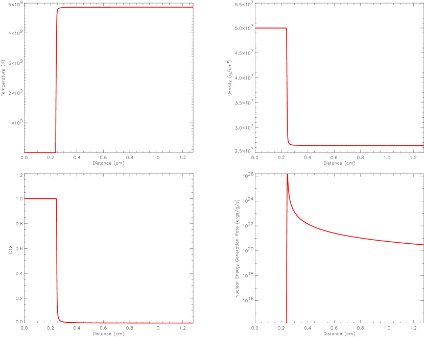
Figure 17.— Flame structure for a planar $5\times 10^{7}\ \mathrm{g\ cm^{-3}}$ pure carbon CF88 flame. Shown are temperature (top left), density (top right), carbon mass fraction (bottom left), and nuclear energy generation rate (bottom right).

An accurate description of the deflagration speed requires resolving the front. For all the flames studied here, we ran with several different resolutions, in order to find out how much resolution was necessary for the flame speed and width to converge. Table 5 summarizes the results of one such resolution study, for the $1\times 10^{8}\ \mathrm{g\ cm^{-3}}$ pure carbon flame. We see that 20-40 zones in the flame width is sufficient to determine the flame speed accurately. The main calculations in this paper were run with a resolution that put about 20 computational zones in the flame width ($l_{f}^{0(I)}$). We did not consider simulations with less than 5 zones in the flame width.

Appendix B CONSERVATIVE INTERPOLATION

In FLASH, the computational zones are organized into blocks, typically containing 8-16 uniformly gridded zones in each coordinate direction. Adapting to the flow is achieved by allowing blocks to vary in resolution by a factor of two with respect to neighboring blocks. When a region needs to be refined, the parent block is cut in half in each dimension, creating $2^{d}$ new blocks, where $d$ is the dimensionality. Initializing the newly created zones in each child block requires that we reconstruct the zone-average data in the parent (and its neighbors) and use this to compute the child data in a conservative fashion. This method is also needed at jumps in resolution, when exchanging guardcell information between neighboring blocks.

Reconstruction is achieved by fitting a quadratic polynomial to the parent data. Since Flash a finite-volume code, the coefficients of the interpolation polynomial must be chosen to reproduce the zone average values of the parents in the stencil. Figure 18 shows the three coarse zones used to initialize the children.

Figure 18.— Schematic showing three coarse zones with zone-averaged data $\left<f\right>_{i-1}$, $\left<f\right>_{i}$, and $\left<f\right>_{i+1}$ (top). The $i$-th zone is refined to create two children (shown on bottom), whose data is to be initialized with $\left<f\right>_{ic}$ and $\left<f\right>_{ic+1}$, through conservative interpolation.

Given the polynomial,

$$f(r)=a_{1}r^{2}+a_{2}r+a_{3}\enskip,$$ (B1)

we apply the constraints,

$$\frac{4\pi}{V_{i}}\int_{r_{i-1/2}}^{r_{i+1/2}}r^{2}drf(r)=\left<f\right>_{i}\enskip,$$ (B2)

to each of the parent zones and solve to find $a_{1}$, $a_{2}$, and $a_{3}$. Here, $V_{i}$ is the volume of the zone, which, for spherical coordinates, is

$$V_{i}=\frac{4}{3}\pi(r_{i+1/2}^{3}-r_{i-1/2}^{3})\enskip,$$ (B3)

and $\left<f\right>_{i}$ is the average value of variable $f$ in zone $i$. The zone edges are denoted by half-integer indices, as illustrated in Figure 18. This polynomial can then be integrated over the children to initialize their data. It is also used when filling guardcells at coarse-fine interfaces.

Applying Eq. B2 to the $i$-th zone yields

$$\frac{3}{5}a_{1}\raisebox{-2.15277pt}{\LARGE$\Theta$}_{3}^{5}\,r_{i}+\frac{3}{4}a_{2}\raisebox{-2.15277pt}{\LARGE$\Theta$}_{3}^{4}\,r_{i}+a_{3}=\left<f\right>_{i}$$ (B4)

where, for notational convenience, we define the operator

$$\raisebox{-2.15277pt}{\LARGE$\Theta$}_{n}^{m}\,r_{i}\equiv\frac{r_{i+1/2}^{m}-r_{i-1/2}^{m}}{r_{i+1/2}^{n}-r_{i-1/2}^{n}}$$ (B5)

We also use the $i-1$ and $i+1$ zones, and get

$$\frac{3}{5}a_{1}\raisebox{-2.15277pt}{\LARGE$\Theta$}_{3}^{5}\,r_{i-1}+\frac{3}{4}a_{2}\raisebox{-2.15277pt}{\LARGE$\Theta$}_{3}^{4}\,r_{i-1}+a_{3}=\left<f\right>_{i-1}$$ (B6)

$$\frac{3}{5}a_{1}\raisebox{-2.15277pt}{\LARGE$\Theta$}_{3}^{5}\,r_{i+1}+\frac{3}{4}a_{2}\raisebox{-2.15277pt}{\LARGE$\Theta$}_{3}^{4}\,r_{i+1}+a_{3}=\left<f\right>_{i+1}$$ (B7)

Equations B4–B7 can be solved for $a_{1}$, $a_{2}$, and $a_{3}$ to yield:

$$a_{2}=\frac{4}{3}\frac{\left[\raisebox{-2.15277pt}{\LARGE$\Theta$}_{3}^{5}\,r_{i}-\raisebox{-2.15277pt}{\LARGE$\Theta$}_{3}^{5}\,r_{i+1}\right]\left(\left<f\right>_{i}-\left<f\right>_{i-1}\right)-\left[\raisebox{-2.15277pt}{\LARGE$\Theta$}_{3}^{5}\,r_{i}-\raisebox{-2.15277pt}{\LARGE$\Theta$}_{3}^{5}\,r_{i-1}\right]\left(\left<f\right>_{i}-\left<f\right>_{i+1}\right)}{\left[\raisebox{-2.15277pt}{\LARGE$\Theta$}_{3}^{4}\,r_{i}-\raisebox{-2.15277pt}{\LARGE$\Theta$}_{3}^{4}\,r_{i-1}\right]\left[\raisebox{-2.15277pt}{\LARGE$\Theta$}_{3}^{5}\,r_{i}-\raisebox{-2.15277pt}{\LARGE$\Theta$}_{3}^{5}\,r_{i+1}\right]-\left[\raisebox{-2.15277pt}{\LARGE$\Theta$}_{3}^{4}\,r_{i}-\raisebox{-2.15277pt}{\LARGE$\Theta$}_{3}^{4}\,r_{i+1}\right]\left[\raisebox{-2.15277pt}{\LARGE$\Theta$}_{3}^{5}\,r_{i}-\raisebox{-2.15277pt}{\LARGE$\Theta$}_{3}^{5}\,r_{i-1}\right]}\enskip,$$ (B8)

$$a_{1}=\frac{5}{3}\frac{1}{\left[\raisebox{-2.15277pt}{\LARGE$\Theta$}_{3}^{5}\,r_{i}-\raisebox{-2.15277pt}{\LARGE$\Theta$}_{3}^{5}\,r_{i+1}\right]}\left\{\left<f\right>_{i}-\left<f\right>_{i+1}-\frac{3}{4}a_{2}\left[\raisebox{-2.15277pt}{\LARGE$\Theta$}_{3}^{4}\,r_{i}-\raisebox{-2.15277pt}{\LARGE$\Theta$}_{3}^{4}\,r_{i+1}\right]\right\}\enskip,$$ (B9)

and

$$a_{3}=\left<f\right>_{i}-\frac{3}{5}a_{1}\raisebox{-2.15277pt}{\LARGE$\Theta$}_{3}^{5}\,r_{i}-\frac{3}{4}a_{2}\raisebox{-2.15277pt}{\LARGE$\Theta$}_{3}^{4}\,r_{i}\enskip.$$ (B10)

Together with Eq. B1, these reconstruct the data in the $i$-th zone. When we refine, two children are created from the $i$-th zone, each taking up half the interval. This is illustrated in Figure 18 on the lower axis. For convenience, we use $ic$ to refer to the child index space, with $r_{ic-1/2}=r_{i-1/2}$, as shown in the figure. The child data is found by integrating Eq. B1 over the child zone as

$$\left<f\right>_{ic}=\frac{4\pi}{V_{ic}}\int_{r_{ic-1/2}}^{r_{ic+1/2}}r^{2}drf(r)\enskip,$$ (B11)

where $ic$ refers to the child zone index. Carrying out the integration, we find the value of the child data, in terms of the parent data and it’s immediate neighbors is

$$\left<f\right>_{ic}=\frac{3}{5}a_{1}\raisebox{-2.15277pt}{\LARGE$\Theta$}_{3}^{5}\,r_{ic}+\frac{3}{4}a_{2}\raisebox{-2.15277pt}{\LARGE$\Theta$}_{3}^{4}\,r_{ic}+a_{3}\enskip.$$ (B12)

This procedure is guaranteed to be conservative, but not guaranteed to be monotonic. If monotonicity is a requirement, then we can check whether the newly initialized child data falls outside the limits of the coarse zones in the stencil, and if so, fall back to direct insertion.

Appendix C MODEL FLAMES

In this appendix, we describe methods and results for ‘model’ flames, both to connect with the combustion literature and to provide simpler models for understanding the astrophysical flames.

C.1. Equation Of State

For the simple model flames we use a ideal gas gamma-law equation of state

$$P=(\gamma-1)\rho\epsilon\enskip,$$ (C1)

supplemented with an expression relating the temperature and the pressure (ideal gas approximation),

$$P=\frac{N_{a}k}{\bar{A}}\rho T\enskip,$$ (C2)

where $\epsilon$ is the internal energy / gram, $N_{a}$ is Avogadro’s number, $k$ is Boltzmann’s constant, and $\bar{A}$ is the average atomic mass of the mixture of fluids. For the model flames, we use $\gamma=5/3$.

C.2. Diffusion

For some of our model flames, we allow finite $\mathrm{Le}$, and so species diffusion is also calculated. Here, the diffusion term of the species evolution equation is

$$\frac{\partial\rho X_{i}}{\partial t}=\nabla\cdot(D_{s}\nabla\rho X_{i}),$$ (C3)

where $X_{i}$ is the mass fraction of species $i$, and $D_{s}$ is the species diffusivity. When species diffusion is included, $D_{s}$ is assumed constant and fixed. The species diffusion is solved in the same way as the thermal diffusion, described in § 3.3.

C.3. Burning

In § 3.5.1, we described the burning rates for the astrophysical flames. Here we describe simpler burning rates used for the model flames.

C.3.1 KPP

A simple burning mechanism, often used by applied mathematicians because it is tractable analytically, is due to Kolmogorov et al. (1937), known for the authors of that paper as KPP. It is a one-step reaction that irreversibly converts fuel to ash:

$$\frac{d\Theta}{dt}=-\frac{dX_{f}}{dt}=a\Theta X_{f}$$ (C4)

where $\Theta$ is a linearly scaled temperature such that $\Theta=1$ corresponds to the temperature of the burned ash, and $\Theta=0$ corresponds to the temperature of the unburned fuel. The concentration (mass fraction) of fuel is given by $X_{f}$, also varying from 0–1. An arbitrary parameter $a$ sets the rate of reaction.

Along with $a$ and the diffusivities $D_{th}$ and $D_{s}$, we have another parameter we can choose — the energy input of the burning with respect to the background energy. We parameterize this by the ratio of the energy released by burning a gram of material to the thermal energy of a gram of fuel in the unburned state

$$q\equiv\frac{\Delta e/(\mu_{f})}{C_{P}T_{u}},$$ (C5)

where $\Delta e$ is the binding energy released by burning a single particle of fuel, $\mu_{f}$ its mass, and $C_{P}$ is the heat capacity at constant pressure of the fuel.

C.3.2 Arrhenius

Real flames, both astrophysical and terrestrial, have such strongly peaked temperature dependencies that their structure can be approximately be broken up into a diffusive “preheat” zone, where reactions are negligible, and a thin reaction zone, where most of the burning occurs and the temperature is roughly constant. Model flames using a KPP burning rate lack this important feature, because of KPP’s fairly gentle temperature dependence.

Thus, as a more realistic model, we consider an Arrhenius rate (see for example Williams 1985)

$$\frac{dT}{dt}=aT_{a}\rho^{n}X_{f}^{m}e^{-T_{a}/T},$$ (C6)

where $T_{a}$ is an ‘activation temperature’ large compared to any of the temperatures in the system. If the molecular weights of the fuel and ash are the same, then in terms of $X_{f}$ this becomes

$$\frac{dX_{f}}{dt}=-a\frac{T_{a}}{qT_{u}}\rho^{n-1}X_{f}^{m}e^{-T_{a}/T}.$$ (C7)

C.4. Results

For the scale-free model flames, dimensional values of parameters are somewhat arbitrary. Parameters were chosen so that the fastest outward-propagating spherical flames would have $dr_{f}/dt\approx 1$ in a domain where the slowest sound speed would be $c_{s}=100$, and all flames were run with these parameters. $D_{th}$ was fixed at $0.0625~{}\mathrm{cm^{2}\ s^{-1}}$, and $D_{s}=D_{th}/\mathrm{Le}$. The unburned state was set to $T_{u}=0.1,\rho_{u}=1.$ and the energy release was set so that $T_{b}^{0}=0.64$. The atomic weight of both the fuel and ash were set to 1385.1.

We consider two sets of flames — ‘KPP flames’, which have an ideal gas EOS and burn with the KPP burning rate described in §C.3.1, and ‘Arrhenius flames’, which also use the ideal gas EOS but burn with an Arrhenius law, described in §C.3.2. Simulations were run with varying temperature dependence and Lewis numbers. Simulations with finite large Lewis numbers become computationally increasingly expensive, as an increasingly smaller species diffusion zone must be resolved adequately.

C.4.1 KPP flames

Results for KPP flames are shown in Fig 19. Shown are results from simulations with $a=0.3$, $\mathrm{Le}=1$, and $a=0.3$, $\mathrm{Le}=\infty$. Data from outwardly-propagating and inwardly-propagating spherical flames, and planar flames are shown. Quantitative results are summarized in Table 6. The resolution used was that chosen in the Appendix for the $\mathrm{Ze}\sim 5$, $\mathrm{Le}=\infty$ flame, although the KPP flames are much thicker.

Figure 19.— Flame speed versus $\mathrm{Ka}_{T}/l_{f}$ for KPP flames, with $\mathrm{Le}=1$ (left) and $\mathrm{Le}=\infty$ (right). For each graph, data points for positive $\mathrm{Ka}_{T}/l_{f}$ are from simulations of a spherically expanding flame, data points for $\mathrm{Ka}_{T}/l_{f}=0$ are for a planar flame, and those for negative $\mathrm{Ka}_{T}/l_{f}$ are for a spherical flame propagating inwards.

$\mathrm{Le}$	$S_{l}^{0}$ (cm s-1)	$l_{f}^{0(I)}$ (cm)	$l_{f}^{0(II)}$ (cm)	${\cal{L}_{M}}^{(+)}$ (cm)		${\cal{L}_{M}}^{(-)}$ (cm)
1	$0.0896$	$5.43$	$4.42$	$-.533$  ±	.139	$+1.28$  ±	.60
$\infty$	$0.0927$	$5.31$	$4.23$	$-.604$  ±	.139	$+1.92$  ±	.82

Table 6KPP flame data.

We use the $\dot{\epsilon}_{\mathrm{nuc}}$-based method for flame velocities as described in §4.4, even though the approximation of a thin reaction front is a poor one for these KPP flames. The quantitative results shown here can be changed significantly by choosing the flame position differently within the burning zone of the flame; the errors quoted for ${\cal{L}_{M}}$ in Table 6 come from using the approximate $\pm 1\ \mathrm{cm}$ uncertainty in flame position shown in Fig. 3.

We see here that KPP flames do not behave in a way described by the Markstein relation. Although the negatively and positively strained flames separately respond significantly and linearly to strain, the sign of the response is different in the two cases. Straining the KPP flames here result in a slowing down of the flame, regardless of the sign of the strain.

That the KPP flame responds differently to strain rates of order a flame crossing time than other flame models is easily understood. Where the astrophysical flames described in §2 have a distinct burning and preheat region, the KPP flames do not. Thus, in this case, the straining stretches not just the preheat zone — essentially the preconditioning for the burning zone — but the burning zone itself.

C.4.2 Arrhenius flames

Arrhenius flames were run with $\mathrm{Ze}\sim 5$ and 8. The flame structures for $\mathrm{Ze}\sim 5$ planar flames with different Lewis numbers are shown in Fig. 20; $\mathrm{Le}=\infty$ flames with positive, zero, and negative strain are shown in Fig. 21. The plots of flame speed versus scaled dimensionless strain are shown in Fig. 22 and Fig. 23. Table 7 gives the quantitative results from these flames. Quoted errors on ${\cal{L}_{M}}$ come from uncertainties in the best fit. The $\mathrm{Le}=\infty$, $\mathrm{Ze}\sim 8$ flame proved too difficult to reliably ignite with the constant diffusivity used here.

Figure 20.— Shown is the flame structure (solid line is scaled $\dot{\epsilon}_{\mathrm{nuc}}$, dashed line is $X_{f}$, and dotted temperature) for planar Arrhenius $\mathrm{Ze}\sim 5$ flames, with $\mathrm{Le}=1,2,5,\infty$ at the top left, top right, bottom left, and bottom right. $\dot{\epsilon}_{\mathrm{nuc}}$ is scaled to 81434.6 ergs g^-1 s^-1, and temperature to the adiabatic temperature of the $\mathrm{Le}=\infty$ flame, $T_{b}^{0}=0.64$. As the species diffusion decreases, the size of the location where there is both enough heat and fuel to burn decreases, and the burning zone narrows considerably, increasing peak $\dot{\epsilon}_{\mathrm{nuc}}$ (although the total burning rate only changes by a factor of 2.) X-axis is distance into the unburned material from the flame position $r_{f}$.

Figure 21.— Shown is the flame structure (solid line is scaled $\dot{\epsilon}_{\mathrm{nuc}}$, dashed line is $X_{f}$, and dotted temperature) for Arrhenius $\mathrm{Ze}\sim 5$ flames which are the outward propagating (top), planar (middle), and inward propagating (bottom). $\mathrm{Ka}_{T}/l_{f}$ is $+.2625\ \mathrm{cm^{-1}}$ for the outward propagating flame, $0\ \mathrm{cm^{-1}}$ for the planar flame, and $-.03675\ \mathrm{cm^{-1}}$ for the inward flame. Although the change in the thermal and fuel structure is very small, the flame speed changes by $\sim 10\%$.

Figure 22.— Flame speed versus $\mathrm{Ka}_{T}/l_{f}$ for $\mathrm{Ze}\sim 5$ Arrhenius flames. Shown are plots for $\mathrm{Le}=1$ (top left), $\mathrm{Le}=2$ (top right), $\mathrm{Le}=5$ (bottom left), and $\mathrm{Le}=\infty$ (bottom right). For each graph, data points for positive $\mathrm{Ka}_{T}/l_{f}$ are from simulations of a spherically expanding flame, data points for $\mathrm{Ka}_{T}/l_{f}=0$ are for a planar flame, and those for negative $\mathrm{Ka}_{T}/l_{f}$ are for a spherical flame propagating inwards.

Figure 23.— Flame speed versus $\mathrm{Ka}_{T}/l_{f}$ for $\mathrm{Ze}\sim 8$ Arrhenius flames. Shown are plots for $\mathrm{Le}=1$ (top left), $\mathrm{Le}=2$ (top right), and $\mathrm{Le}=5$ (bottom). For each graph, data points for positive $\mathrm{Ka}_{T}/l_{f}$ are from simulations of a spherically expanding flame, data points for $\mathrm{Ka}_{T}/l_{f}=0$ are for a planar flame, and those for negative $\mathrm{Ka}_{T}/l_{f}$ are for a spherical flame propagating inwards.

$\mathrm{Ze}$	$\mathrm{Le}$	$S_{l}^{0}$ (cm s-1)	$l_{f}^{0(I)}$ (cm)	$l_{f}^{0(II)}$ (cm)	${\cal{L}_{M}}$ (cm)		$\mathrm{Ma}^{(I)}$	$\mathrm{Ma}^{(II)}$
5.37	1	0.0227	$1.547$	$0.827$	$+0.452$  ±	0.003	$+.292$	$+.546$
	2	0.0269	$1.344$	$0.694$	$-0.195$  ±	0.001	$-.150$	$-.281$
	5	0.0330	$1.078$	$0.5528$	$-0.434$  ±	0.002	$-.403$	$-.823$
	$\infty$	0.0399	$0.8906$	$0.4233$	$-0.347$  ±	0.001	$-.334$	$-.702$
8.06	1	0.0204	$1.636$	$1.481$	$+0.909$  ±	0.002	$+0.555$	$+0.614$
	2	0.0248	$1.326$	$0.5422$	$-0.297$  ±	0.001	$-0.224$	$-0.548$
	5	0.0326	$1.025$	$0.4052$	$-0.654$  ±	0.001	$-0.638$	$-1.614$

Table 7Arrhenius flame data.

The Arrhenius flames response to strain is linear, and the Markstein lengths are of order the flame thickness or smaller. The sign of the response is negative for $\mathrm{Le}=\infty$ flames, as expected. The sign changes for smaller Lewis number as the effect of fuel diffusion into the ash, which acts in the opposite direction of the thermal diffusion into the fuel, becomes more significant.

One sees in these results and in the astrophysical results that flame response to negative curvature is noisier than that to positive curvature. This is caused by the physical setup of the simulations. For the ingoing flames, pressure waves caused by ignition transients can be trapped inside the spherical flame due to the density jump at the flame’s position. In our 1-d simulations, the pressure waves bounce along the interior of the flame. The waves bounce off of the reflecting boundary condition, correctly modelling the same wave coming from the part of the spherical domain on the other side of the origin. The pressure waves are only amplified as the flame moves inwards. This is shown on the left of Fig. 24 for the $\mathrm{Le}=5$, $\mathrm{Ze}\sim 5$ ingoing Arrhenius flame. On the right of Fig. 24 is plotted the same values for the corresponding outward-propagating flame. Here, the transient pressure waves can largely leave the domain.

Figure 24.— Scaled pressure fluctuation ($(P-P_{0})/P_{0}$) in the computational domain, with scaled $\dot{\epsilon}_{\mathrm{nuc}}$ to show the flame’s position, for an inward-propagating $\mathrm{Ze}\sim 5$, $\mathrm{Le}=5$ Arrhenius flame on the left, and the corresponding outward-propagating flame on the right. Pressure waves can be trapped inside the flame (eg., in the unburned fuel) for the inward flame, and amplified as the flame moves inwards; these fluctuations in the fuel state lead to the observed scatter in burning rates. The pressure waves are largely able to leave the domain in the outward-propagating case, causing reduced scatter.

The pressure fluctuations, while small ($\approx 0.2\%$ for the ingoing flames, and $\approx 0.02\%$ for the outgoing flames), are enough to slightly modify the local burning, leading to the observed scatter in measured burning velocities. As the temperature sensitivity of the flame increases, the noise caused by the same pressure fluctuations become larger; this explains the increased noise in the $\mathrm{Ze}\sim 8$ flames.

References

- Arnett & Livne (1994a) Arnett, D., & Livne, E. 1994a, ApJ, 427, 315
- Arnett & Livne (1994b) —. 1994b, ApJ, 427, 330
- Aung et al. (1997) Aung, K. T., Hassan, M. I., & Faeth, G. M. 1997, Comb. and Flame, 109, 1
- Aung et al. (1998) —. 1998, Comb. and Flame, 112, 1
- Bevington (1969) Bevington, P. R. 1969, Data Reduction and Error Analysis for the Physical Sciences (New York: McGraw-Hill Book Company)
- Blinnikov & Sasorov (1996) Blinnikov, S. I., & Sasorov, P. V. 1996, Phys. Rev. E, 53, 4827
- Blinnikov et al. (1995) Blinnikov, S. I., Sasorov, P. V., & Woosley, S. E. 1995, Space Science Reviews, 74, 299
- Bradley et al. (1996) Bradley, D., Gaskell, P. H., & Gu, X. J. 1996, Comb. and Flame, 104, 176
- Bradley et al. (1998) Bradley, D., Hicks, R. A., Lawes, M., Sheppard, G. W., & Wooley, R. 1998, Comb. and Flame, 115, 126
- Bychkov & Liberman (1995a) Bychkov, V. V., & Liberman, M. A. 1995a, A&A, 302, 727
- Bychkov & Liberman (1995b) —. 1995b, ApJ, 451, 771
- Calder (2002) Calder, A. C. et al.. 2002, ApJS, 143, 201
- Caughlan & Fowler (1988) Caughlan, G. R., & Fowler, W. A. 1988, Atomic Data and Nuclear Data Tables, 40, 283
- Chung & Law (1988) Chung, S. H., & Law, C. K. 1988, Comb. and Flame, 72, 325
- Clanet & Searby (1998) Clanet, C., & Searby, G. 1998, Phys. Rev. Lett., 80, 3867
- Clavin & Williams (1982) Clavin, P., & Williams, F. A. 1982, J. Fluid Mech., 116, 251
- Colella & Glaz (1985) Colella, P., & Glaz, H. M. 1985, J. Comp. Phys., 59, 264
- Colella & Woodward (1984) Colella, P., & Woodward, P. R. 1984, J. Comp. Phys., 54, 174
- Denet (1998) Denet, B. 1998, Combust. Theory Modelling, 2, 167
- Domínguez & Höflich (2000) Domínguez, I., & Höflich, P. 2000, ApJ, 528, 854
- Fryxell (2000) Fryxell, B. et al.. 2000, ApJS, 131, 273
- Gamezo et al. (2003) Gamezo, V. N., Khokhlov, A. M., Oran, E. S., Chtchelkanova, A. Y., & Rosenberg, R. O. 2003, Science
- Glassman (1996) Glassman, I. 1996, Combustion, 3rd edn. (San Diego: Academic Press)
- Groot et al. (2002) Groot, G. R. A., van Oijen, J. A., de Goey, L. P. H., Seshadri, K., & Peters, N. 2002, Combust. Theor. Model., 6, 675
- Gu et al. (2000) Gu, X. J., Haq, M. Z., Lawes, M., & Wooley, R. 2000, Comb. and Flame, 121, 41
- Hassan et al. (1998) Hassan, M. I., Aung, K. T., & Faeth, G. M. 1998, Comb. and Flame, 115, 539
- Hecht (1987) Hecht, E. 1987, Optics, 2nd edn. (Reading, Massachusetts: Addison-Wesley Publishing Company)
- Hedstrom (1979) Hedstrom, G. W. 1979, J. Comp. Phys., 30, 222
- Helenbrook & Law (1998) Helenbrook, B. T., & Law, C. K. 1998, Comb. and Flame, 117, 155
- Hillebrandt & Niemeyer (2000) Hillebrandt, W., & Niemeyer, J. C. 2000, ARA&A, 38, 191
- Karpov et al. (1997) Karpov, V. P., Lipatnikov, A. N., & Wolanski, P. 1997, Comb. and Flame, 109, 436
- Khokhlov (1991a) Khokhlov, A. M. 1991a, A&A, 245, 114
- Khokhlov (1991b) —. 1991b, A&A, 245, L25
- Khokhlov (1995) Khokhlov, A. M. 1995, ApJ, 449, 695
- Kolmogorov et al. (1937) Kolmogorov, A. N., Petrovskii, I. G., & Piskunov, N. S. 1937, Bull. Moskov. Gos. Univ. Mat. Mekh, 1, 1
- Kwon & Faeth (2001) Kwon, O., & Faeth, G. 2001, Comb. and Flame, 124, 590
- Landau & Lifshitz (1987) Landau, L. D., & Lifshitz, E. M. 1987, Fluid Mechanics, 2nd edn. (Oxford: Pergamon Press)
- Law & Sung (2000) Law, C. K., & Sung, C. J. 2000, Progress in Energy and Combustion Science, 459
- MacNeice et al. (2000) MacNeice, P., Olson, K. M., Mobarry, C., deFainchtein, R., & Packer, C. 2000, Computer Physics Communications, 126, 330
- Markstein (1964) Markstein, G. H. 1964, Nonsteady Flame Propagation (New York: Pergamon Press)
- Matalon & Matkowsky (1982) Matalon, M., & Matkowsky, B. J. 1982, J. Fluid Mech., 124, 239
- Müller et al. (1997) Müller, U. C., Bollig, M., & Peters, N. 1997, Comb. and Flame, 108, 349
- Niemeyer & Hillebrandt (1995) Niemeyer, J. C., & Hillebrandt, W. 1995, ApJ, 452, 779
- Niemeyer et al. (1996) Niemeyer, J. C., Hillebrandt, W., & Woosley, S. E. 1996, ApJ, 471, 903
- Nomoto et al. (1984) Nomoto, K., Thielemann, F.-K., & Yokoi, K. 1984, ApJ, 286, 644
- Reinecke et al. (1999) Reinecke, M., Hillebrandt, W., & Niemeyer, J. C. 1999, A&A, 347, 739
- Reinecke et al. (2002a) —. 2002a, A&A, 386, 939
- Reinecke et al. (2002b) —. 2002b, A&A, 391, 1167
- Röpke et al. (2003) Röpke, F. K., Niemeyer, J. C., & Hillebrandt, W. 2003, ApJ, in press
- Sedov (1959) Sedov, L. I. 1959, Similarity and Dimensional Methods in Mechanics (New York: Academic Press)
- Sun et al. (1999) Sun, C. J., Sung, C. J., He, L., & Law, C. K. 1999, Comb. and Flame, 118, 108
- Thompson (1987) Thompson, K. W. 1987, J. Comp. Phys., 68, 1
- Timmes (2000) Timmes, F. X. 2000, ApJ, 528, 913
- Timmes & Swesty (2000) Timmes, F. X., & Swesty, F. D. 2000, ApJS, 126, 501
- Timmes & Woosley (1992) Timmes, F. X., & Woosley, S. E. 1992, ApJ, 396, 649
- Williams (1985) Williams, F. A. 1985, Combustion Theory, 2nd edn. (Menlo Park, California: Benjamin/Cummings Publishing Company)
- Woosley et al. (1984) Woosley, S. E., Axelrod, T. S., & Weaver, T. A. 1984, in ASSL Vol. 109: Stellar Nucleosynthesis, 263
- Zeldovich et al. (1985) Zeldovich, Y. B., Barenblatt, G. I., Librovich, V. B., & Markhviladze, G. M. 1985, The Mathematical Theory of Combustion and Explosions (New York: Consultants Bureau)
- Zeldovich & Frank-Kamenetskii (1938) Zeldovich, Y. B., & Frank-Kamenetskii, D. A. 1938, Zh. Fiz. Khim, 12, 100
- Zingale (2001) Zingale, M. et al.. 2001, in Relativistic Astrophysics: 20th Texas Symposium, 490