Cluster Lensing of QSOs as a Probe of $\Lambda$CDM and Dark Energy Cosmologies

Abstract

Wide-separation lensed QSOs measure the mass function and evolution of massive galaxy clusters, in a similar way to the cluster mass function deduced from X-ray–selected samples or statistical measurements of the Sunyaev–Zeldovich effect. We compute probabilities of strong lensing of QSOs by galaxy clusters in dark energy cosmologies using semianalytical modelling and explore the sensitivity of the method to various input parameters and assumptions. We highlight the importance of considering both the variation of halo properties with mass, redshift and cosmology and the effect of cosmic scatter in halo concentration. We then investigate the extent to which observational surveys for wide-separation lensed QSOs may be used to measure cosmological parameters such as the fractional matter density $\Omega_{M}$, the $\it{rms}$ linear density fluctuation in spheres of $8$ h^-1 Mpc, $\sigma_{8}$, and the dark energy equation of state parameter $w$.

We find that wide-separation lensed QSOs can measure $\sigma_{8}$ and $\Omega_{M}$ in an equivalent manner to other methods such as cluster abundance studies and cosmic shear measurements. In assessing whether lensing statistics can distinguish between values of $w$, we conclude that at present the uncertainty in the calibration of $\sigma_{8}$ in quintessence models dominates the conclusions reached. Nonetheless, lensing searches based on current QSO surveys such as the Two-degree Field and the Sloan Digital Sky Survey with $10^{4}$–$10^{5}$ QSOs should detect systems with angular separations $\Delta\theta>5^{\prime\prime}$ and hence can provide an important test of the standard cosmological model that is complementary to measurements of cosmic microwave background anisotropies.

1 Introduction

The first year Wilkinson Microwave Anisotropy Probe (WMAP) measurements (Spergel et al., 2003) of the cosmic microwave background anisotropy seem to confirm that the universe is flat and that there is a sufficient density of “dark energy” to accelerate the expansion of the universe. It is not yet clear whether the dark energy is a cosmological constant which is spatially uniform and constant with time, or instead a dynamic cosmic field, so-called quintessence, which varies in space and time. A combination of the WMAP observations with other astronomical datasets has provided a good measurement of the dark energy equation of state parameter $w<-0.78$ ($95\%$ confidence limit) (Spergel et al., 2003). However, the combination of datasets in this way means that independent tests of both the values of cosmological parameters and the underlying assumptions cannot be made. Statistical tests based on the abundance of massive structures can be an alternative test of the standard cosmological model in which structures have grown with the expansion of the Universe from initially Gaussian primordial fluctuations. Observational signatures of clusters at $z\loa 3$ contrast with observations of the cosmic microwave background anisotropies at $z\approx 1000$, forming a complementary cosmological probe. One well-known example of such a test is the statistics of strong lensing events.

This paper investigates the use of strong lensing statistics as probes of cosmology, and in particular discusses the joint constraints that may be obtained on the equation of state of the dark energy, $P=w\rho$ (where in this paper $w$ is assumed constant), and on the fractional matter density $\Omega_{M}$ and power spectrum normalisation, parameterised by $\sigma_{8}$, the $\it{rms}$ linear density fluctuation in spheres of $8$ h^-1 Mpc. Multiple images of distant QSOs can be produced by strong lensing by intervening mass overdensities such as galaxies and clusters of galaxies. The work presented in this paper is focused on wide-separation lensed QSOs, $\Delta\theta\goa 5^{\prime\prime}$. These systems are produced by structures with the mass of clusters of galaxies, so wide-separation lensed QSOs can probe the number and evolution of clusters in a similar way to the cluster mass function deduced from X-ray–selected samples or statistical measurements of the Sunyaev–Zeldovich effect. However, these latter methods depend on emission from, or scattering by, the baryons in a cluster, while gravitational lensing directly probes its mass. But, despite the existence of arcminute-separated multiple images of background galaxies (Smail et al. 1995; Kneib et al. 1996; Sahu et al. 1998), the detection of wide-separation lensed QSOs has proved to be a hard task. Only two systems are known to have separations $\Delta\theta>5^{\prime\prime}$: $Q0957+561$, with $\Delta\theta=6.26^{\prime\prime}$ and redshift $z=1.41$, is the widest-separation confirmed lensed QSO known (Walsh, Carswell $\&$ Weymann, 1979) and $RX\,J0921+4529$, with $\Delta\theta=6.97^{\prime\prime}$ and $z=1.65$, remains a wide-separation lens candidate (Muñoz et al., 2001). Other systematic lensing searches (Ofek et al., 2001; Maoz et al., 1997; Phillips et al., 2001; Phillips, Browne $\&$ Wilkinson, 2001) have failed to find wide-separation lensed QSOs. Ongoing redshift surveys such as the Two-Degree Field QSO Redshift Survey (2QZ) and the Sloan Digital Sky Survey (SDSS) with $10^{4}$–$10^{5}$ QSOs might be able to detect wide separation lensed systems. Miller et al. (2002) have reported evidence for QSO lensed candidates with arcminute separations selected from 2QZ, but further observational work is required to demonstrate that those candidates are indeed strongly lensed systems.

Strong lensing statistics have been calculated for $\Lambda$CDM models by Li $\&$ Ostriker (2002) and for QCDM models by Sarbu et al. (2001). The work presented here not only extends the work performed by Sarbu et al. (2001) to wide-separation lenses but also uses what we consider to be more accurate assumptions about the halo mass function and the mass distribution within halos, and investigates more explicitly the effect of making differing model assumptions. First, we adopt the Sheth $\&$ Tormen (Sheth et al., 2001) halo mass function, which should more accurately predict the mass function of massive clusters. Second, we utilise the dark matter halo concentration prescription of Eke et al. (2001) and take into account the variation of the concentration with redshift, mass and cosmology. Here we have explicitly considered the dependence of the concentration on $w$, $\Omega_{M}$ and $\sigma_{8}$. For comparison with previous work, Sarbu et al. (2001) used the Bullock et al. (2001) relation and only considered the mass and redshift dependence of concentration. Third, we include the effects of scatter in halo concentration (Bullock et al., 2001) which was neglected by Li $\&$ Ostriker (2002) and Sarbu et al. (2001). These last points are crucial as lensing depends very strongly on halo concentration, in that more concentrated halos are more efficient lenses. We also note that the statistics of strong lensing events depends critically on the assumed value of $\sigma_{8}$, and by assuming an empirical relationship between $\sigma_{8}$ and $w$ the cause of variation in lensing statistics with cosmological parameters can become obscured. In fact the Sarbu et al. (2001) results are dominated by the assumed $\sigma_{8}$–$w$ relationship. In this paper we present results as a function of $\sigma_{8}$, $w$ and $\Omega_{M}$ so that the inter-relationships between these variables may be understood. We also show how calculation of the amplification bias changes when widely separated multiple images are being considered.

Hence, in section 2 we describe how the lensing probability arising from massive clusters may be estimated and discuss the elements that play a role in that computation, in section 3 we show the results of that analysis and in section 4 we discuss the outlook for being able to constrain cosmological parameters from such measurements.

2 The Lensing Probability

If we define the lens system with a lens at redshift $z$, a source at redshift $z_{S}$, which is in our case a QSO, the probability for the source being lensed with an image separation greater than $\Delta\theta$ is:

$$P(z_{S},>\Delta\theta)=\int_{0}^{z_{S}}(1+z)^{3}\frac{dr}{dz}\,dz\,\int_{M_{min}}^{\infty}\frac{dn}{dM}(M,z)\,dM\,\sigma_{lens}$$ (1)

where $\sigma_{lens}$ is the lensing cross-section which is specified in section 2.3, $n$ is the number of lenses per comoving volume, $M_{min}$ is the minimum mass required to produce an image splitting $\Delta\theta$, $r$ is the proper cosmological distance to the lens and $(1+z)^{3}$ accounts for the fact that $n$ is in units of comoving volume. The basic ingredients that take part in the calculation of the lensing probability are therefore the halo mass function, the background cosmology and the lens cross-section which depends critically on the halo profile and on the magnification bias. The following subsections will detail these ingredients.

2.1 The Cosmological Model

We consider spatially flat cosmological models with a dark energy equation of state $P_{Q}=w\rho_{Q}$, where $P_{Q}$ is the pressure, $\rho_{Q}$ is density and $w$, the so-called dark energy equation of state parameter, is assumed to be constant with time. In this case the local energy conservation law (see e.g Peebles $\&$ Ratra 2002) is $\dot{\rho}_{Q}=-3\left(\ddot{a}/a\right)\rho_{Q}\left(1+w\right)$, where $\rho_{Q}\propto a^{-3(1+w)}$ and $a$ is the cosmic expansion factor. Dark energy has a number of implications in cosmology and some of these are of direct relevance for strong lensing. Two clear consequences are the effects on the cosmic volume and the growth of structure. For a flat model with fixed fractional matter density $\Omega_{M}$ (and therefore $\Omega_{Q}=1-\Omega_{M}$) the cosmic volume per unit redshift decreases as $w$ increases whereas structures start forming earlier if $w$ increases (Bartelmann et al., 2002; Klypin et al., 2003). For our purposes we need to compute angular diameter distances. In flat dark energy cosmologies the angular diameter distance from an object at redshift $z_{1}$ to an object at redshift $z_{2}$ is given in units of $c/H_{0}$ by:

$$D_{z_{1},z_{2}}=\frac{1}{(1+z_{2})}\int_{z_{1}}^{z_{2}}\frac{dz}{(\Omega_{M}(1+z)^{3}+\Omega_{Q}(1+z)^{3(1+w)})^{0.5}}.$$ (2)

Other consequences of dark energy such as its influence on the mass power spectrum, the linear and non-linear overdensity for collapse and the dark matter halo concentrations will be discussed in later sections. We adopt a value for Hubble’s constant, $H_{0}=70$ km s^-1 Mpc^-1.

2.2 The Halo Mass Function

In this paper we consider lensing only by massive galaxy clusters, and neglect any contribution from individual galaxies. The results obtained should be valid on image separation scales where the calculated lensing probability significantly exceeds that due to individual galaxies, and from our analysis we estimate the minimum scale to be $\Delta\theta\sim 5^{\prime\prime}$. To calculate the number density and redshift distribution of massive clusters we adopt the Sheth $\&$ Tormen (Sheth et al., 2001) mass function. This is a modified version of that obtained by the Press-Schechter formalism (Press $\&$ Schechter, 1974) that fits better the space density of high-mass halos determined from N-body simulations. This increase in precision is obtained principally by introducing an additional factor into the critical linear overdensity for collapse, where that factor is adjusted so that the mass function matches the results from those simulations. This mass function produces results almost indistinguishable from the mass function of Jenkins et al. (2001), which is also a fit to N-body simulations. Both fitting formulae predict significantly greater numbers of high-mass halos than Press-Schechter. In adopting this function, we implicitly have to assume that the function is valid for dark energy models as indicated by the simulations of Klypin et al. (2003). The mass function is primarily a single-parameter modification of Press-Schechter: the latter makes no assumption about background cosmology, and already fits remarkably well to results from N-body simulations. We can be confident that the mass function prescription will remain valid for a wide range of cosmological models, although we shall argue later that it is important to test not only the mass function but also the distribution of halo concentration values by N-body simulation (e.g. Klypin et al. 2003).

We also adopt the linear growth and the linear matter power spectrum for QCDM models obtained by Ma et al. (1999). The major difference between the power spectra of the $\Lambda$CDM and QCDM models is that dark energy may cluster spatially on scales corresponding to wavenumbers $k\loa 0.01h$ Mpc^-1, whereas the cosmological constant remains spatially smooth on all length scales. This signifies that the QCDM power spectrum on cluster scales has the same shape as the $\Lambda$CDM model but has a different large-scale shape, and, especially if the normalisation is determined from large-scale CMB measurements, the overall amplitude is changed (Ma et al., 1999). Here we use the Bardeen et al. (1986) fitting formula for the $\Lambda$CDM model transfer function with the modification of Sugiyama (1995) in order to account for the baryons. The resulting $\Lambda$CDM power spectra are extremely close to those computed by Eisenstein $\&$ Hu (1999).

To avoid varying too many parameters, we fix the primordial power spectrum index to be $n=1$ and the baryon density to be the WMAP best-fit value of $\Omega_{b}=0.047$. In fact, varying the primordial index does not change significantly the halo mass function if it is normalised to a particular value of $\sigma_{8}$. Modifying the power spectrum to include the effects of baryons in fact decreases the lensing probability, somewhat contrary to our initial expectations: this point will be discussed again in the context of halo concentrations.

One critical quantity that varies with $w$ is the linear theory critical threshold for collapse of a halo, which is a key part of the Press-Schechter and Sheth-Tormen prescriptions. We adopt the fitting function proposed by Weinberg $\&$ Kamionkowski (2002) which was modelled after Kitayama $\&$ Suto (1996): in fact the value of the linear theory critical threshold for the collapse at the typical redshift of the lens ($z\sim 0.5$) does not vary considerably, not more than approximately $5$ per cent, over a wide range of $\Omega_{M}$ and $w$. Figs 1 and 2 present the Sheth $\&$ Tormen mass function as a function of halo mass. As is well known, the mass function is a steep function of mass, decreases with redshift and increases exponentially with $\sigma_{8}$. Fig. 2 shows the dependence of the mass function on $\sigma_{8}$ and $\Omega_{M}$. Fig. 1 plots the mass function at two redshifts, $z=0.1$ and $z=1$ for a cosmological model with a cosmological constant and for a model with a dark energy equation of state parameter $w=-0.5$. Clearly, the mass function is not very sensitive to the dark energy equation of state parameter at $z=0.1$ but the difference between the two models is greater at higher redshifts, and the model with $w=-0.5$ predicts more halos than the cosmological constant model, for a fixed value of $\sigma_{8}$, as shown also by Klypin et al. (2003).

Figure 1: The Sheth & Tormen mass function and its (lack of) sensitivity to the dark energy equation of state parameter $w$. Thin lines are for $z=0.1$ and thick lines are for $z=1.0$. Solid lines correspond to a cosmological constant model with $w=-1.0$ and dashed lines correspond to a quintessence model with $w=-0.5$. The fractional matter density and the power spectrum normalisation were set to $\Omega_{M}=0.3$ and $\sigma_{8}=0.9$ respectively.

Figure 2: The Sheth & Tormen mass function and its sensitivity to $\Omega_{M}$ and $\sigma_{8}$. The solid line is for $(\sigma_{8},\Omega_{M})=(0.8,0.3)$, the dashed line for $(\sigma_{8},\Omega_{M})=(0.9,0.3)$ and the dash-dotted line for $(\sigma_{8},\Omega_{M})=(0.9,0.2)$. Here, the mass function is computed at $z=0$ and we assume $w=-1.0$.

2.3 The Lensing Cross Section

The lensing cross section, which may be defined as the area on the lens plane for which multiple imaging occurs, is given by:

$$\sigma_{lens}=D_{L}^{2}\int_{0}^{\beta_{crit}(z,M)}2\;\pi\,\beta\;A(z,M,\beta)\;d\beta$$ (3)

where $D_{L}$ is the angular diameter distance from the observer to the lens, $\beta$ is the angle between the lens and the source, $\beta_{crit}(z,M)$ is the critical angle for multiple imaging and $A(z,M,\beta)$ is the amplification bias. Note here that the amplification bias is part of the integrand and is therefore explicitly computed as a function of the angle $\beta$ instead of simply calculating the cross section as $\sigma_{lens}=\pi(D_{L}\beta_{crit})^{2}$ as in previous studies.

2.3.1 The Halo Profile

Following previous lensing probability calculations, we assume that the lenses have a circularly symmetric surface mass density, $\Sigma({\bf r})=\Sigma(\left|{\bf r}\right|)$, where ${\bf r}$ is a two-dimensional position vector in the lens plane. In this case, the lens equation reduces to a one-dimensional form (Maoz et al., 1997; Schneider et al., 1992):

$$\beta=\frac{D_{LS}}{D_{S}}\alpha(\theta)-\theta$$ (4)

where $\beta$ is the angle between the lens and the source, $D_{LS}$ is the angular diameter distance between the lens and the source, $D_{S}$ is the angular diameter distance between the observer and the source, $\theta$ is the angle between the lens and the lensed image formed and $\alpha$ is the deflection angle:

$$\alpha(r)=\frac{4GM(<r)}{c^{2}r}$$ (5)

where $M(<r)$ is the projected mass enclosed within radius $r$ and is given by:

$$M(<r)=2\pi\int_{0}^{r}\Sigma(r^{\prime})r^{\prime}dr^{\prime}.$$ (6)

We discuss the possible effects of departures from smooth, circularly-symmetric lenses in section 4.

The density profile of the lenses is modelled with the NFW profile (Navarro, Frenk $\&$ White, 1997) which appears to be a good fit to numerically simulated halos over a wide range of masses in various cosmological scenarios. The density profile is:

$$\rho(r)=\frac{\rho_{S}}{\frac{r}{r_{S}}(1+\frac{r}{r_{S}})^{2}}$$ (7)

where $\rho_{S}$ and $r_{S}$ are the characteristic density scale and scale radius, respectively. This profile is steeper than the singular isothermal sphere at large radii but is flatter at smaller radii. Moore et al. (1999) simulations prefer a steeper inner profile although the observational evidence for the formation of radial arcs in clusters (Sand et al., 2002) is favouring a shallower inner profile. The inner slope is thus an issue under debate and we will not discuss it here but we point out that the lensing probability is rather sensitive to its value (Li $\&$ Ostriker, 2002): lensing probability increases as the inner slope steepens because for standard NFW profiles the projected mass density is usually lower than the critical density for lensing for all but the innermost radii of a cluster.

The surface mass density of the NFW profile is (Bartelmann, 1996):

$$\Sigma(x)=\frac{2\rho_{S}r_{S}}{x^{2}-1}f(x)$$ (8)

where $x$ is the radial coordinate in units of scale radius $x\equiv\frac{r}{r_{S}}$. As a result the bend angle takes the form:

$$\alpha(x)=\frac{16\pi\rho_{S}r^{2}_{s}}{c^{2}}\frac{g(x)}{x}$$ (9)

where g(x) is (Bartelmann, 1996):

$$g(x)=\int_{0}^{x}\frac{yf(y)}{y^{2}-1}dy.$$ (10)

In order to calculate the lensing cross section it is convenient to calculate a critical angle for lensing, $\beta_{crit}$. Multiple imaging occurs if and only if the angle $\beta$ satisfies $|\beta|\leq\beta_{crit}$ where $\beta_{crit}$ is the solution of $d\beta/d\theta=0$. In the case of perfect alignment between the observer, circularly-symmetric lens and source, $\beta=0$, and $|\beta|<\beta_{crit}$ there are three images formed, for $|\beta|=\beta_{crit}$ two images and for $|\beta|>\beta_{crit}$ only one image is formed. Non-circularly symmetric lenses can produce more than three images. A key question for the lensing cross section is how to calculate the inner parameters $\rho_{s}$ and $r_{s}$ and their variation with mass, redshift and cosmological model. These parameters can be related to the virial parameters of the halo through the halo concentration parameter. The latter is basically a measurement of the relative size of the core with respect to the virial radius. Here we adopt the approach of calculating the halo concentration from prescriptions based on N-body simulations.

2.3.2 Dark Matter Halo Concentrations

Formally, the mass of the NFW profile diverges, so to define the mass we adopt the standard formalism of calculating the mass within the virial radius $R_{vir}$ of a sphere with density $\Delta_{vir}$ times the critical density $\rho_{crit}$:

$$M_{vir} = 4\pi\int_{0}^{R_{vir}}\rho r^{2}dr=4\pi\rho_{S}r^{3}_{s}f(c_{vir})$$ (11)

$$= \frac{4\pi}{3}\Delta_{vir}\rho_{crit}(z)R_{vir}^{3}$$

where $f(c_{vir})=\ln(1+c_{vir})-\frac{c_{vir}}{1+c_{vir}}$ and we define the halo concentration parameter as $c_{vir}=\frac{R_{vir}}{r_{S}}$. $\Delta_{vir}$ is the non-linear overdensity at virialisation. With these definitions we can compute the scale radius $r_{s}=R_{vir}/c_{vir}$ and the characteristic density $\rho_{S}$:

$$\rho_{s}=\frac{\Delta_{vir}}{3}\rho_{crit}(z)\frac{c_{vir}^{3}}{f(c_{vir})}.$$ (12)

In the work that follows we take into account the variation of the mean halo concentration with redshift, halo mass and cosmology, and in particular with $w$. The assumptions on these dependencies turn out to make a significant difference to the overall lensing probabilities: Li $\&$ Ostriker (2002) had no dependence of concentration on mass in their $\Lambda$CDM analysis. Sarbu et al. (2001) included the redshift and mass variation in their QCDM studies but did not include any dependence on $w$, assuming instead the values appropriate for a $\Lambda$CDM cosmology. To evaluate those dependencies we adopt the concentration prescription of Eke et al. (2001). That prescription is based around the premise that halo concentration increases as the redshift of formation of a dark halo increases, a reflection of the higher matter density at earlier epochs. A characteristic redshift of formation that varies with the shape of the power spectrum is calculated and a value for a single parameter can be found which yields concentration values that match well the results from N-body simulations for a wide range of cosmological models, and has been tested against the original NFW results for masses up to $10^{15}M_{\sun}$. Concentrations deduced in this way seem to be generally in broad agreement with values measured from fitting to the X-ray profiles of clusters over the range $10^{14}\loa M_{vir}\loa 10^{16}M_{\sun}$ (e.g. Wu $\&$ Xue 2002). It does appear that the dependence on mass in those samples may be steeper than predicted, but X-ray selection of clusters is likely to have some effect on the observed relationship, and at high masses, which are most important for wide-separation lensing, comparable concentration values are obtained from the measurements and from the Eke et al. (2001) prescription.

In this paper we extend the Eke et al. (2001) prescription in a natural way to accommodate dark energy models working under the assumption that the algorithms derived from numerical simulations in $\Lambda$CDM models are also valid in QCDM models. We have used the fitting function of Weinberg $\&$ Kamionkowski (2002), modelled after Kitayama $\&$ Suto (1996) for the non-linear overdensity at virialisation, $\Delta_{vir}$, which increases with $w$. This arises because structures start forming earlier in models with a higher $w$, the mean energy in a collapsing object is larger and hence a higher overdensity for virialisation is required (Weinberg $\&$ Kamionkowski, 2002).

Figure 3: Dark matter halo concentrations function for four different combinations of redshift and dark energy equation of state parameter $(z,w)$. The fractional matter density and the power spectrum normalisation were set to $\Omega_{M}=0.3$ and $\sigma_{8}=0.9$ respectively. Thin lines are for $z=0.1$, thick lines for $z=1.0$. Solid lines correspond to a $\Lambda$CDM model ($w=-1.0$) and dashed lines correspond to a quintessence model with $w=-0.5$.

Figure 4: Dark matter halo concentrations for three ($\sigma_{8}$,$\Omega_{M}$) combinations. The solid line is for $(\sigma_{8},\Omega_{M})=(0.8,0.3)$, the dashed line for $(\sigma_{8},\Omega_{M})=(0.9,0.3)$ and the dash-dotted line for $(\sigma_{8},\Omega_{M})=(0.9,0.2)$. Concentrations were computed at $z=0.$ and assumed a $\Lambda$CDM model.

Figures 3 and 4 show the concentrations obtained for differing cosmological models. The concentrations decrease with the mass of the halo since high halo masses are formed later in structure formation models. In quintessence models structures form earlier than in $\Lambda$CDM, resulting in higher concentrations for a given mass. This trend is evident in the plot of Fig. 3. Although the Eke et al. (2001) prescription has not yet been exhaustively tested for $w$ models, comparison with the dark energy simulations of Klypin et al. (2003) show good general agreement, with higher $w$ models exhibiting higher concentrations for a given mass. Fig. 4 presents concentrations for three combinations of ($\sigma_{8}$,$\Omega_{M}$). An increase in $\sigma_{8}$ makes the halo concentrations higher and a decrease in $\Omega_{M}$ lowers the concentrations.

One key additional factor to consider is the scatter in halo concentration values about the mean relations computed above. The numerical simulations show that there is a scatter in the concentration values which may be associated with a spread in collapse epochs and/or formation histories (Bullock et al. 2001; Wechsler et al. 2002). This scatter has a dramatic effect on the wide-separation lensing probability because clusters with NFW profiles and moderate concentration values have surface mass densities which only rise above the critical density for lensing at small radii. Even a 30 percent increase in concentration can bring the mass density above the critical value over a substantially larger range of radii, thereby greatly increasing the lensing probability at large separations. So giving a minority of the cluster halo population larger concentrations than the mean produces a significant increase in lensing probability, as discussed in section 3. The scatter also reduces the differences between the various models however, as also discussed later in this paper. The amount of scatter measured from N-body simulations depends critically on which halos are chosen for study: relaxed halos are better fit by NFW profiles and have a moderate scatter. Bullock et al. (2001) argue that the scatter appears to have log-normal distribution with $\sigma_{c}=0.18$ and we incorporate this distribution into the computation of the lensing probability. Finally we note that the Eke et al. (2001) prescription has been tested in a range of power spectra shapes. Here we find that introducing $\Omega_{b}=0.047$ lowers the mean halo concentrations and therefore results in a decrease of the lensing probability.

2.3.3 The Amplification Bias

The effect of the amplification bias on the lensing cross section, $A(z,M,\beta)$, is to boost the lensing probability because sources that are intrinsically dimmer than the flux limit of the survey $f_{lim}$ are brought into the sample by the magnification. If the source QSOs have a single power-law flux distribution with redshift-independent slope $\alpha$, $N_{z_{S}}(>f)=f^{-\alpha}$ then the amplification bias is given by:

$$A(z,M,\beta) = \frac{N_{z_{S}}(>f_{lim}/\mu(z,M,\beta))}{N_{z_{S}}(>f_{lim})}$$ (13)

$$= \mu^{\alpha}(z,M,\beta)$$

where $\mu$ is the magnification factor which for circularly symmetric lenses is given by:

$$\mu = \left|\frac{\theta}{\beta}\right|\left|\frac{d\theta}{d\beta}\right|$$ (14)

$$= \left|\frac{\theta}{\beta}\right|\left|\left(\frac{D_{LS}}{D_{S}}\frac{d\alpha(\theta)}{d\theta}-1\right)^{-1}\right|.$$

In order to calculate the magnification factor we need to solve the lens equation and obtain the three (or two) solutions. In surveys for wide-separation lensed systems, where the image separation is larger than the survey resolution, the multiple images are separately detected and we need to compute the probability that at least two images will appear brighter than the survey flux selection limit. Hence the relevant quantity to compute is the amplification of the second-brightest of the multiple images. This approach differs from that commonly taken in which multiple images are assumed to be unresolved and the amplification bias is calculated from the sum of the fluxes of the lensed images. In addition, in this paper we compute both the magnification factor and the minimum mass required to produce a given image splitting as a function of the angle $\beta$, in contrast to the usually-followed procedure of calculating the minimum mass for lensing assuming perfect alignment between the observer, the lens and the source.

3 Results

Figure 5: The lensing cross section as a function of $w$ for a halo of mass $M_{Halo}=10^{14}M_{\odot}$ and redshift $z=0.3$. The QSO is at redshift $z_{QSO}=1.5$. Curves are for three different $(\sigma_{8},\Omega_{M})$ combinations. Solid curves are for $\Omega_{M}=0.3$ and $\sigma_{8}=0.8$, dashed for $\Omega_{M}=0.3$ and $\sigma_{8}=0.9$ and dash-dotted curves for $\Omega_{M}=0.2$ and $\sigma_{8}=0.9$. No amplification bias has been applied. Thin lines show the lensing cross section $\sigma_{lens}=\pi(D_{L}\beta_{crit})^{2}$. Thick lines include the additional effect of introducing the scatter in the halo concentrations.

Figure 6: The minimum mass required to lens a QSO at redshift $z_{QSO}=1.5$ with image separation $\Delta\theta=10^{\prime\prime}$. The lens is at redshift $z_{Lens}=0.3$ and it is assumed that there is close to perfect alignment, $\beta\approx 0$. The minimum mass is plotted as a function of $w$ for three pairs of $(\sigma_{8},\Omega_{M})$. The thin solid line is for $(\sigma_{8},\Omega_{M})=(0.8,0.3)$, the thick solid is for $(\sigma_{8},\Omega_{M})=(0.9,0.3)$ and the dashed line is for $(\sigma_{8},\Omega_{M})=(0.9,0.2)$.

Having explored the sensitivity of the mass function and the dark matter halo concentrations to the dark energy equation of state parameter as well as to the fractional matter density and the power spectrum normalisation, we now investigate the influence of the same cosmological parameters on the remaining lensing ingredients, such as the lensing cross section and the minimum mass for lensing.

We first look at the lensing cross section: in order to separate the various effects we do not at this stage apply the magnification bias, and hence effectively calculate $\sigma_{lens}=\pi(D_{L}\beta_{crit})^{2}$. Fig. 5 shows that the lensing cross section increases monotonically in quintessence universes for fixed $\sigma_{8}$, and the amplitude of the cross section is larger if the power spectrum normalisation is raised. This arises because the concentrations are larger in those cases which in turn make lensing more efficient. If the matter content is decreased from $\Omega_{M}=0.3$ to $\Omega_{M}=0.2$ the cross section is lowered, although the difference between the models decreases for higher values of $w$. This occurs because halo concentrations are in fact lower for lower values of $\Omega_{M}$ (see Fig. 4). Also shown is the additional effect of including a scatter in the value of the concentrations, in particular by assuming the log-normal distribution with $\sigma_{c}=0.18$. Including the scatter significantly increases the lensing cross section: for example, in a model with $(\sigma_{8},\Omega_{M})=(0.9,0.3)$ and $w=-1$ its value is raised by a factor of approximately one hundred, as the tail of high concentration halos dominates the statistics. We should expect that for large scatter in halo concentration the differences between cosmological models should be reduced (assuming the scatter itself is independent of cosmology) and this is reflected also in Fig. 5. Concentration scatter was not included in previous work by Sarbu et al. (2001) and Li $\&$ Ostriker (2002).

The other key ingredient on the lensing calculation is the minimum mass required to produce multiple imaging and this is included in formula 1 as the lower limit of the mass integral. This is generally calculated assuming perfect alignment between the lens, observer and the source, that is to say with $\beta=0$. For the lensing probabilities here we actually compute the minimum mass as a function of the angle $\beta$ but in order to analyse how its value varies with cosmological parameters we assume $\beta=0$. Fig. 6 shows that the minimum mass required to lens a QSO at redshift $z_{QSO}=1.5$ with an image separation $\Delta\theta=10^{\prime\prime}$ and a lens redshift $z_{lens}=0.3$ clearly decreases with $w$ and $\sigma_{8}$. For $\sigma_{8}=0.9$ the minimum mass required is greater for a universe with a lower fractional matter density.

Figure 7: The lensing probability as a function of image separation $\Delta\theta$ for four different values of the slope of the QSO number-counts. The solid line shows $\alpha=0$, corresponding to no amplification bias. The fractional matter density and the power spectrum normalisation were set to $\Omega_{M}=0.3$ and $\sigma_{8}=0.9$ respectively. The dark energy equation of state parameter was set to $w=-1$.

Figure 8: The lensing probability as a function of source redshift, $z_{QSO}$, for three different image separations: $\Delta\theta=5^{\prime\prime}$ (top line), $\Delta\theta=10^{\prime\prime}$ (middle line) and $\Delta\theta=30^{\prime\prime}$ (bottom line), assuming $\Omega_{M}=0.3$, $\sigma_{8}=0.9$ and $w=-1$.

We can now look at the probability distribution of image separations (Figs 7 and 10). There is a clear and steep fall of the probability toward higher image separations which is a consequence of a mass function that falls off quite rapidly combined with a higher required minimum mass for lensing events with larger separations. Here we underline the sensitivity of the lensing probability to the slope of the source number-counts. Fig. 7 shows the expected behaviour: a steeper slope favours higher lensing rates. Note that if magnification bias is not accounted for then the lensing probability is reduced by a factor of about ten. At faint radio and optical selection levels, with $B\goa 20$, the slope of the QSO number-counts are significantly flatter than Euclidean, although because we need to know the slope at flux levels fainter than the unlensed limit for the survey being searched for lensed QSOs the actual value of $\alpha$ is often uncertain. The observed apparent slope for the 2QZ optical QSO survey has value $\alpha\approx 0.8$ at faint magnitudes, although this value does not take account of sample incompleteness. Hereafter we shall assume a slope $\alpha=1$: to first order the change in lensing probability resulting from assuming a different value for $\alpha$ may be estimated from Fig. 7.

Assumptions about the typical source redshift and the distribution of source redshifts also affect the lensing probability. Fig. 8 shows that the lensing optical depth is a steep function of source redshift: if a source is moved from redshift $z=1.5$ to $z=2.5$, the lensing probability is increased by approximately a factor of three. This behaviour is also found in estimates of the lensing optical depth for giant arcs (Wambsganss, Bode $\&$ Ostriker, 2003). Fig. 8 shows that applying an accurate estimate of the median source redshift is essential. But we also expect that a distribution of source redshifts about the median would increase the lensing probability, and indeed if we adopt the redshift distribution of the 2QZ 10K catalogue (Croom et al., 2001) we find that the lensing probability is increased by approximately 10$\%$.

Figure 9: The lensing probability as a function of concentration scatter, $\sigma_{c}$, for three different image separations: $\Delta\theta=5^{\prime\prime}$ (top line), $\Delta\theta=10^{\prime\prime}$ (middle line) and $\Delta\theta=30^{\prime\prime}$ (bottom line), assuming $\Omega_{M}=0.3$, $\sigma_{8}=0.9$ and $w=-1$.

Uncertainties in halo concentrations which can be expressed by $\sigma_{c}$ can also alter the lensing probability. This is shown in Fig. 9: if the scatter in halo concentrations is changed from $0.18$ (the value assumed in our analysis) to $0.4$ the lensing probability is increased by a factor of six. Therefore, an accurate value of the scatter in halo concentrations is fundamental.

The effect of increasing $w>-1$ on the probability distribution of image separations is to boost the integrated lensing probability. The difference between the models increases for larger $w$ (Fig. 10). This is partly owing to halo concentrations being larger in quintessence models, making the lensing cross section higher, and partly owing to the minimum mass required for multiple imaging decreasing with $w$ (Fig. 6): the mass function of galaxy clusters falls sufficiently steeply that the small decrease in mass has a significant effect.

Figure 10: The lensing probability as a function of image separation $\Delta\theta$ for four different values of $w$ in a flat universe with $\sigma_{8}=0.9$ and $\Omega_{M}=0.3$.

Fig. 11 explores the sensitivity of the lensing probability to $\Omega_{M}$ and $\sigma_{8}$ for differing minimum values of separation, $\Delta\theta=10^{\prime\prime}$ and $\Delta\theta=30^{\prime\prime}$. The latter probability is about ten times smaller than the former. We confirm the expected increase of probability with $w$ as in Fig. 10 and note that the probability also increases with $\sigma_{8}$. Indeed the lensing cross section increases with $\sigma_{8}$ and the minimum mass for lensing also decreases with this cosmological parameter. In addition, there is an exponential rise of the mass function with its value. The overall effect is therefore an increase of the lensing probability. When we lower $\Omega_{M}$ from 0.3 to 0.2 the probability decreases.

Figure 11: The probability of a QSO at redshift $z_{QSO}=1.5$ being lensed with an image separation bigger than $\Delta\theta$ in a quintessence model. The sensitivity of the probability to $\sigma_{8}$ and $\Omega_{M}$ is also shown. Solid lines are for $\Omega_{M}=0.3$ and $\sigma_{8}=0.8$. Dashed lines are for $\Omega_{M}=0.3$ and $\sigma_{8}=0.9$ and dash-dotted lines are for $\Omega_{M}=0.2$ and $\sigma_{8}=0.9$. Thick lines correspond to a minimum image separation of $\Delta\theta=30^{\prime\prime}$ and thin lines correspond to $\Delta\theta=10^{\prime\prime}$.

There are evident cosmological parameter degeneracies and those are clearly shown on the contour plots provided in Figs 12 and 13. One has to bring in other independent cosmological constraints in order to break the degeneracies. In Fig. 12 we overplot the best-fit result from the abundance of rich galaxy clusters obtained by Wang $\&$ Steinhardt (1998) and Lokas et al. (2003) as well as the constraint obtained from the COBE measurement of the cosmic microwave background (Ma et al. 1999; Bunn $\&$ White 1997). In Fig. 13 we show the constraints from a study of the present-day number density of galaxy clusters (Allen et al., 2003) and from a cosmic shear measurement (Hoekstra, Yee and Gladders, 2002). Jarvis et al. (2002) and Pierpaoli et al. (2001) review the variation found in these measurements from studies performed by other groups. The WMAP best-fit result is also shown (Spergel et al., 2003).

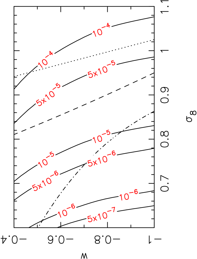
Figure 12: Contours of probability $P(z_{QSO}=1.5,\Delta{\theta}>10^{\prime\prime})$ in the $w-\sigma_{8}$ plane for a universe with fractional matter density $\Omega_{M}=0.3$. The dashed and dotted lines show the constraints from cluster abundances as obtained by Wang $\&$ Steinhardt (1998) and Lokas et al. (2003), respectively. The dashed-dotted line shows the result of COBE power spectrum normalisation (Ma et al., 1999).

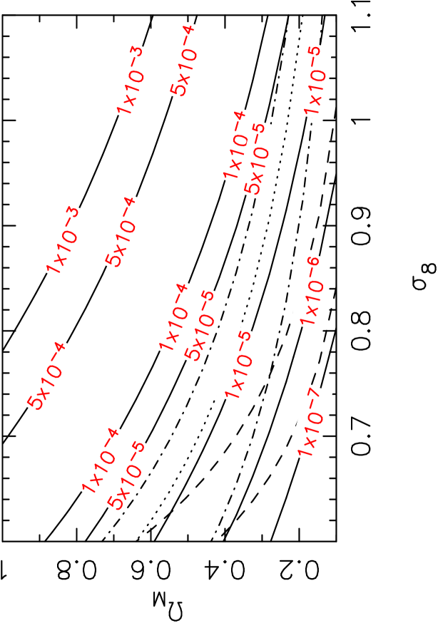
Figure 13: Contours of probability $P(z_{QSO}=1.5,\Delta{\theta}>10^{\prime\prime})$ in the $\sigma_{8}-\Omega_{M}$ plane for a universe dominated by a cosmological constant ($w=-1$). The area enclosed by the dashed lines represents the constraints from the study of the local cluster abundance (Allen et al., 2003). The area enclosed by the dot-dashed lines shows the constraints obtained from the cosmic shear measurement of Hoekstra, Yee and Gladders (2002). The dotted line is the WMAP relation (Spergel et al., 2003).

The ability of surveys to actually discriminate between cosmological models will depend on survey size and on the numbers of detected lenses of course. As an illustration, we assume a survey of $10^{5}$ sources containing four lensed sources with $\Delta\theta>5^{\prime\prime}$, which corresponds to the model prediction for a flat cosmological model with $w=-1$, $\sigma_{8}=0.9$ and $\Omega_{M}=0.3$, and the source redshift distribution of the 2QZ 10K catalogue (Croom et al., 2001). The likelihood function chosen depends on the number of lenses as

$$L=\frac{\lambda^{N}e^{-\lambda}}{N!}$$

where $\lambda$ is the expected number of lensed systems and $N$ is the actual number observed; we do not here consider information contained in the distribution of angular separations. Fig. 14 shows the $68.3$ and $95.4$ per cent confidence level contours in the $\sigma_{8}-\Omega_{M}$ plane. Fig. 15 shows the constraints on $w$ when one assumes $\Omega_{M}=0.3$ and $\sigma_{8}=0.9$ (marginalising over the current uncertainty in $\sigma_{8}$ would significantly broaden the likelihood function). The confidence intervals are somewhat broader than can be attained from current generations of cosmic microwave background, weak lensing measurements or deductions from cluster abundance measurements, but it is important to note that these methods are all complementary tests of the cosmological model. The CMB measurements probe the Universe at $z\sim 1000$; cluster abundance determinations are dependent on correct modelling of thermal emission from baryons in cluster potential wells; cosmic shear measures the mean fluctuations in matter density on Mpc scales; the abundance of strong lensing events measures the extreme high-mass tail of the mass function, with a small number of lensed systems being generated by the most extreme objects. In the final analysis the abundance of strong lensing events may tell us more about the formation of the most massive structures in the universe than about the values of cosmological parameters.

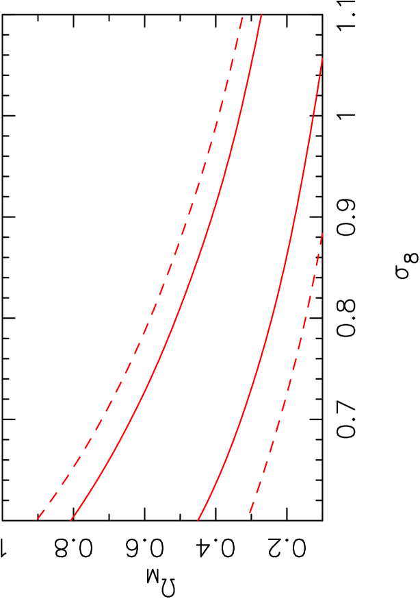
Figure 14: The $68.3$ (solid line) and $95.4$ (dashed line) per cent confidence level contours on $\sigma_{8}$ and $\Omega_{M}$ (assuming $w=-1.$) obtained for a survey of $10^{5}$ sources, four of which are lensed with $\Delta\theta>5^{\prime\prime}$.

Figure 15: The $68.3$ ($w<-0.66$) and $95.4$ ($w<-0.51$) per cent confidence level likelihood constraints on $w$ (assuming $\Omega_{M}=0.3$ and $\sigma_{8}=0.9$) obtained for a survey of $10^{5}$ sources, four of which are lensed with $\Delta\theta>5^{\prime\prime}$.

4 Discussion and Conclusions

We have calculated cluster lensing probabilities of QSOs in dark energy models. The lensing probabilities have been explored over a wide range of angular separations and we have taken into account the cosmology, mass and redshift dependence of halo concentration, while assuming that the algorithms derived from dark matter halo simulations in $\Lambda$CDM models remain valid in QCDM models. Ultimately, these algorithms should be tested against numerical simulations in dark energy cosmologies, but simulations to date indicate that these prescriptions are at least approximately correct (Klypin et al., 2003). What issues remain that could still have an important effect on the predictions of this type of modelling? At this stage we may be reasonably confident that the Sheth $\&$ Tormen mass function is sufficiently well tested that it can be considered a robust prescription, but we should be aware that modifications to the fluctuations giving rise to cosmological structure would lead to differing mass functions. As one example, non-Gaussian initial perturbations significantly increase the mass function at high redshifts (Matarrese et al. 2000; Mathis et al. 2003) and we should expect halos of a given mass to have formed at earlier epochs, and hence have higher values of halo concentration.

There is currently some uncertainty about the universality of the NFW profile and about its applicability to lensing studies. Merely by introducing the known scatter in halo concentration we see a significantly non-linear effect on lensing probability. If, in turn, this scatter is greater then the value adopted in this paper ($\sigma_{c}=0.18$) then that will have a great effect in the lensing probability. As we have seen in Fig. 9, if the scatter in halo concentrations is changed from $0.18$ (the value assumed in our analysis) to $0.4$, the lensing probability is increased by a factor of six. Variations in the inner slope of the halo profile would also have a significant effect (Li $\&$ Ostriker, 2002; Oguri, 2003a). There have been claims based on N-body simulations that the inner slope may be steeper than the standard NFW value (Moore et al., 1999), or that its value steepens with mass (Ricotti, 2002), and there is evidence that some clusters at least may have slopes that are flatter than NFW (Sand et al., 2002). Even if there is not a systematic departure from the canonical NFW profile, scatter about that relation could lead to increase in lensing probability in a similar way to that introduced by the scatter in halo concentration. Other effects to be taken into account include the effect of substructure, especially in recently-formed, non-relaxed clusters: this has already been shown to be important for the statistics of extreme giant arcs (Meneghetti et al., 2003a). Finally, the effect of individual galaxies in a cluster may be noticeable on the smallest angular scales discussed in this paper, although present indications are that this is a relatively small effect in giant arc statistics (Meneghetti et al., 2000) and, likewise, the inclusion of a massive cD galaxy in the centre of the cluster does not seem to significantly enhance the lensing cross section for giant arcs (Meneghetti et al., 2003b).

We have also adopted a circularly symmetric lens profile, whereas even relaxed individual clusters are likely to be triaxial. Again, this effect has been shown to be potentially significant for the statistics of extreme giant arcs (Bartelmann et al., 2002; Oguri, 2003b), although it is not yet clear whether there is any significant effect on the statistics of less extreme lensing events.

In applying these models to actual surveys, we should of course also take care to ensure that we are using accurate estimates for the slope of the QSO number-counts and that we take account of the redshift distribution of QSOs. In particular, an accurate estimation of the median redshift of the sources is essential as the lensing probability is a steep function of source redshift. For optical QSO surveys this is known exactly and therefore does not constitute a source of uncertainty. However, for radio surveys the median redshift of the sources can be quite uncertain and therefore provide a systematic error in the lensing probability: if the median redshift is increased from $z=1$ to $z=1.5$ the lensing probability is increased by a factor about three (Fig. 8).

With these caveats, we can use the models produced here to understand what constraints, if any, may be placed on cosmological models as a result of either detecting or not detecting wide-separation lensed QSOs in surveys such as SDSS and 2QZ. Within the cosmic concordance model, a flat model with $\Omega_{M}=0.3$ and a WMAP value of $\sigma_{8}=0.9$ we find that the lensing probability increases with the dark energy equation of state parameter and attribute this effect to the fact that the concentrations of dark matter halos are higher in quintessence models and therefore lenses become more efficient. This effect combined with a mass function that is very steep and a lower minimum mass required for multiple imaging makes more halos available for strong lensing. We also note that the $\sigma_{8}$–$\Omega_{M}$ degeneracy is equivalent to the degeneracy found in other methods such as cluster abundances, cosmic shear measurements and the WMAP analysis (Figs. 13 and  14).

In considering whether lensing statistics can distinguish between values of $w$, we see that at present the uncertainty in the calibration of $\sigma_{8}$ dominates the conclusions reached. Cluster-normalised models predict that lensing probability is not a sensitive indicator of the value of $w$, whereas COBE-normalised values of $\sigma_{8}$ indicate that as $w$ increases, $w>-1$, the expected number of lensing events decreases. Further work is needed to tie down the $\sigma_{8}$ normalisation in $w$ models. Of course, we should not expect cluster- and CMB-determined normalisations to agree except at a single point in parameter space that corresponds to the values for the universe we actually inhabit, but at present we cannot be confident that such a point can be identified. Nonetheless, the determination of the absolute number of lenses at redshifts $z\loa 3$ should provide a good test of the $\Lambda$CDM model, independently of, and in direct contrast with, cosmic microwave background anisotropy measurements at $z\approx 1000$. Alternative methods, such as 3D weak lensing (Heavens, 2003) and weak lensing tomography (Jain $\&$ Taylor, 2003), although at present with current surveys are not able to constrain $w$, potentially offer a more robust probe with an estimated accuracy for $w$ better than $5\%$ for surveys such as the one proposed with the LSST (Jain $\&$ Taylor, 2003).

For a flat cosmological constant model with $\Omega_{M}=0.3$, a WMAP value of $\sigma_{8}=0.9$ and the source redshift distribution of the 2QZ 10K catalogue (Croom et al., 2001), the modelling predicts probabilities of $4.0\times 10^{-5}$, $2.5\times 10^{-5}$ and $4.7\times 10^{-6}$ for lensing events with separations larger than $5^{\prime\prime}$, $10^{\prime\prime}$ and $30^{\prime\prime}$ respectively. This indicates that a survey with $10^{5}$ sources will find approximately 4 lensed QSOs with separations greater than $5^{\prime\prime}$, 2 lensed QSOs with separations greater than $10^{\prime\prime}$ and none with separations greater than $30^{\prime\prime}$. For surveys such as the 2QZ and SDSS the survey selection effects will somewhat alter these numbers. If no wide separation lensed QSOs are detected that would rule out models with high $\sigma_{8}$. Conversely, if large numbers are found, or if any lensed systems significantly larger than $1^{\prime}$ are confirmed, we would need a significant modification to the model presented here, including either significant effects from the presence of substructure or perhaps requiring assumptions in the standard model, such as Gaussianity, to be relaxed. At this stage it would be premature to speculate further. Challenges in the immediate future, then, are to test the expected levels of lensing probabilities against numerical simulations, both to take account of substructure and cluster shape, and to test the predictions in the cases of dark energy models. Joint comparison between multiple image probabilities and the statistics of extreme giant arcs would be a good simultaneous test.

ACKNOWLEDGEMENTS
AML acknowledges the support of the Portuguese Fundação para a Ciência e a Tecnologia.

References

- Allen et al. (2003) Allen S.W., Schmidt R.W., Fabian A.C. Ebeling H., 2003, preprint astro-ph/0208394.
- Bardeen et al. (1986) Bardeen J.M., Bond J.R., Kaiser N. Szalay A.S., 1986, ApJ, 304, 15.
- Bartelmann (1996) Bartelmann M., 1996, AA, 313, 697.
- Bartelmann et al. (2002) Bartelmann M., Meneghetti M., Perrotta F., Baccigalupi C., Moscardini L., 2002, preprint astro-ph/0210066.
- Bartelmann et al. (2002) Bartelmann M., Perrotta F. Baccigalupi C., 2002, AA, 396, 21.
- Bullock et al. (2001) Bullock J.S., Kolatt T.S., Sigad Y., Somerville R.S., Kravtsov, A.V., Klypin, A.A, Primack J.R Dekel A., 2001, MNRAS, 321, 559.
- Bunn White (1997) Bunn E.F. White M., 1997, ApJ, 480, 6.
- Croom et al. (2001) Croom S.M., Smith R.J., Boyle B.J., Shanks T., Loaring N.S., Miller L., Lewis I.J., 2001, MNRAS, 322, L29.
- Eisenstein Hu (1999) Eisenstein D.J. Hu W., 1999, ApJ, 511, 5.
- Eke et al. (2001) Eke V.R., Navarro J.F. Steinmetz M., 2001, ApJ, 554, 114.
- Heavens (2003) Heavens, Alan, 2003, preprint astro-ph/0304151.
- Hoekstra, Yee and Gladders (2002) Hoekstra H., Yee H. Gladders M., 2002, ApJ, 577, 595.
- Jain Taylor (2003) Jain, B. Taylor A., 2003, preprint astro-ph/0306046.
- Jarvis et al. (2002) Jarvis M., Bernstein G.M, Fischer P., Smith D., Jain B., Tyson J.A., Wittman D., 2002, AJ, in press (astro-ph/0210604).
- Jenkins et al. (2001) Jenkins A., Frenk C.S., White S.D.M., Colberg J.M., Cole S., Evrard A.E., Couchman H.M.P. Yoshida N., 2001, MNRAS, 321,372.
- Kitayama Suto (1996) Kitayama T. Suto Y., 1996, ApJ, 469, 480.
- Klypin et al. (2003) Klypin A., Macciò A.V., Mainini R. Bonometto S.A., 2003, preprint astro-ph/0303304.
- Kneib et al. (1996) Kneib J.-P., Ellis R.S., Smail I., Couch W.J. Sharples R.M., 1996, ApJ, 471, 643.
- Kochanek (1995) Kochanek C.S., 1995, ApJ, 453, 545.
- Li Ostriker (2002) Li L.-X. Ostriker J.P., 2002, ApJ, 566, 652.
- Lokas et al. (2003) Lokas E.L., Bode P. Hoffman, 2003, preprint astro-ph/0309485.
- Ma et al. (1999) Ma C.-P., Caldwell R.R., Bode, P. Wang L., 1999, ApJ, 521, L1.
- Maoz et al. (1997) Maoz D., Rix H.W., Gal-Yam, A. Gould, A., 1997, ApJ, 486, 75.
- Mathis et al. (2003) Mathis H., Silk J., Griffiths L.M. Kunz M., 2003, preprint astro-ph/0303519.
- Meneghetti et al. (2003a) Meneghetti M., Bartelmann M. Moscardini L., 2003a, MNRAS, 340, 105.
- Meneghetti et al. (2003b) Meneghetti M., Bartelmann M., Moscardini L., 2003b, preprint astro-ph/0302603.
- Meneghetti et al. (2000) Meneghetti M., Bolzonella M., Bartelmann M., Moscardini L. Tormen G., 2000, MNRAS, 314, 338.
- Miller et al. (2002) Miller L., Lopes A.M., Smith R.J., Croom S.M., Boyle B.J., Shanks T., Outram P., 2002, preprint astro-ph/0210644.
- Moore et al. (1999) Moore B., Quinn T., Governato F., Stadel J. Lake G., 1999, MNRAS, 310, 1147.
- Muñoz et al. (2001) Muñoz J.A., Falco E.E., Kochanek C.S., Lehár J., McLeod B.A., McNamara B.R., Vikhlinin A.A., Impey C.D., Rix H.-W., Keeton C.R., Peng C.Y. Mullis C.R., 2001, ApJ, 546, 769.
- Navarro, Frenk White (1997) Navarro J.F., Frenk C.S. White, 1997, ApJ, 490, 493.
- Matarrese et al. (2000) Matarrese S., Verde L. Jimenez, R., 2000, ApJ, 541, 10.
- Ofek et al. (2001) Ofek E.O., Maoz D., Prada F., Kolatt T. Rix H.-W., 2001, MNRAS, 324, 463.
- Oguri (2003a) Oguri M., 2003, MNRAS, 339, L23.
- Oguri (2003b) Oguri M., Lee J., Suto Y., 2003, preprint astro-ph/0306102.
- Peebles Ratra (2002) Peebles P.J.E., Ratra, B., 2002, preprint astro-ph/0207347.
- Phillips et al. (2001) Phillips P.M., Browne I.W.A., Jackson N.J., Wilkinson P.N., Mao S., Rusin D., Marlow D.R., Snellen I., Neeser M., 2001, MNRAS, 328, 2001.
- Phillips, Browne Wilkinson (2001) Phillips P.M., Browne, I.W.A. Wilkinson P.N., 2001. MNRAS, 321,187
- Pierpaoli et al. (2001) Pierpaoli E., Scott D., White M., 2001, MNRAS, 325, 77.
- Press Schechter (1974) Press W.H. Schechter, P., 1974, ApJ, 187, 425.
- Ricotti (2002) Ricotti M., 2002, preprint astro-ph/0212146.
- Sahu et al. (1998) Sahu K.C., Shaw R.A., Kaiser M.E., Baum S.A., Ferguson H.C., Hayes J.J.E., Gull T.R., Hill R.J., Hutchings J.B., Kimble R.A., Plait P. Woodgate B.E., 1998, ApJ, 492, L125.
- Sand et al. (2002) Sand D.J., Treu T. Ellis R.S., 2002, ApJ, 574, L129.
- Sarbu et al. (2001) Sarbu N., Rusin, D. Ma, C.-P., 2001, ApJ, 561, L147.
- Schneider et al. (1992) Schneider P., Ehlers J., Falco E.E., 1992, Gravitational Lenses (Berlin:Springer).
- Sheth et al. (2001) Sheth R.K., Mo H.J. Tormen G., 2001, MNRAS 323, 1.
- Sheth et al. (2001) Sheth R.K. Tormen G., 1999, MNRAS 308, 119.
- Smail et al. (1995) Smail I., Couch W.J., Ellis R.S. Sharples R.M., 1995, ApJ, 440, 501.
- Spergel et al. (2003) Spergel D.N., et al., 2003, preprint astro-ph/0302209.
- Sugiyama (1995) Sugiyama N., 1995, ApJ Supplement Series, 100, 281.
- Walsh, Carswell Weymann (1979) Walsh D., Carswell R.F. Weymann R.J., 1979, Nature, 279, 381.
- Wambsganss, Bode Ostriker (2003) Wambsganss J., Bode P. Ostriker J., 2003, preprint astro-ph/0306088.
- Wang Steinhardt (1998) Wang L. Steinhardt P.J., 1998, ApJ, 508, 483.
- Wechsler et al. (2002) Wechsler R.H., Bullock J.S., Primack J.R., Kravtsov A.V., Dekel A., 2002, ApJ, 568, 52.
- Weinberg Kamionkowski (2002) Weinberg N.N. Kamionkowski M., 2002, preprint astro-ph/0210134.
- Wu Xue (2002) Wu X.-P. Xue Y.-J., 2000, ApJ, 529, L5.