The Effects of Massive Substructures on Image Multiplicities in Gravitational Lenses

Abstract

Surveys for gravitational lens systems have typically found a significantly larger fraction of lenses with four (or more) images than are predicted by standard ellipsoidal lens models (50% versus 25-30%). We show that including the effects of smaller satellite galaxies, with an abundance normalized by the observations, significantly increases the expected number of systems with more than two images and largely explains the discrepancy. The effect is dominated by satellites with $\sim 20$% the luminosity of the primary lens, in rough agreement with the typical luminosities of the observed satellites. We find that the lens systems with satellites cannot be dropped from estimates of the cosmological model based on gravitational lens statistics without significantly biasing the results.

1 Introduction

While many gravitational lenses can be modeled as single, isolated, massive galaxies, this can only be an approximation. Both the luminosity functions of galaxies and the mass functions of halos derived from hierarchical structure formation predict that massive galaxies are likely to be surrounded by lower mass halos. These halos modify the gravitational potential from that of the central (usually) elliptical galaxy and have several observational consequences. First, the satellite galaxies observed in many systems (e.g. MG0414+0534, Schechter & Moore SchMoo93 (1993); B1030+074, Xanthopoulos et al. xanetal98 (1998); B1152+199, Myers et al. Mye99 (1999), Rusin et al. Rus02 (2002); and B1359+154, Myers et al. Mye99 (1999) for the JVAS/CLASS sample) are required to obtain a successful model of the observed image geometries. The gravitational field produced by an offset nearby satellite is essentially impossible to mimic through variations in the structure of the central lens galaxy or the addition of tidal shears. Second, the satellite galaxies can change the caustic structure of the lens, possibly helping to explain the relatively high numbers of observed quad lenses (e.g. Kochanek & Apostolakis KocApo88 (1988), Rusin & Tegmark, RusTeg01 (2001), Moller & Blain MolBla01 (2001)). Third, even very low mass satellites can perturb the magnification tensors of individual images so as to produce patterns of image magnifications which cannot be reproduced by the central lens galaxy (Mao & Schneider MaoSch98 (1998), Metcalf & Madau MetMad01 (2001), Chiba Chi02 (2002), Dalal & Kochanek DalKoc01 (2002), Schechter & Wambsganss SchWam02 (2002), Keeton Kee03 (2003), Keeton, Gaudi, Petters KeeGauPet02 (2003), Kochanek & Dalal KocDal02 (2002, 2003), Evans & Witt Evans03 (2003)).

In this paper we focus on the second of these effects, the role of substructure in changing the expected numbers of images, in particular the ratio of lenses with 2 or 4 images. Standard statistical models consisting of an isolated elliptical galaxy in an external tidal field have difficulty reproducing the observed ratio of quad to double lenses. In particular, 50% (10 of 20: 10 doubles, 9 quads and 1 with six images) of the published lenses found in the JVAS/CLASS surveys (Patnaik et al. Pat92 (1992), Browne et al. Bro98 (1998, 2002), Wilkinson et al Wil98 (1998), King et al. Kin99 (1999), Myers et al. Mye95 (1995, 1999, 2003)) for lensed flat-spectrum radio sources have more than two images, while the most recent models predict only 24–31% (Rusin & Tegmark, RusTeg01 (2001), hereafter RT). The significance of this “quads to doubles ratio” problem has risen and fallen as the lens sample has grown (see King & Browne KinBro96 (1996), Kochanek 1996b , Keeton, Kochanek & Seljak kks (1997), Finch et al. Fin02 (2002)), but the ratio has always seemed uncomfortably high. Most solutions, other than invocations of bad luck, such as the effects of core radii, high dark matter ellipticities or local tidal fields, are not very successful at changing the ratio without becoming either physically implausible or predicting large numbers of other unobserved image configurations.

Compound lenses have been addressed previously within different approximations. Kochanek & Apostolakis (KocApo88 (1988)) examined the caustic/multiplicity and magnification structure for two lenses of the same mass at differing separations and redshifts. They focused on spherical lenses but indicated modifications which would be introduced by ellipticity as well. Seitz & Schneider (SeiSch92 (1992)) considered multiplicities and magnifications for compound lenses. Moller & Blain (MolBla01 (2001)) calculated probabilities and some characteristic properties for lenses at two different redshifts but they did not consider quantitatively the role of the correlation function in enhancing the numbers of satellites clustered with the primary lens. RT made a limited study of the effects of adding faint SIS (singular isothermal sphere) satellites, concluding that low mass neighbors would have little effect. Here we extend their work to include higher mass neighbors as well (in a sequence of lens mass ratios), the correlation function of galaxies and the number density of satellites. In §2 we outline our calculation. In §3 we discuss the results and how they change when we vary some of our (standard) assumptions. In §4 we summarize the conclusions and outline the issues needing further study.

2 Methodology

We will study the statistical consequences of including a satellite galaxy on the lensing properties of a more massive primary lens. In order to separate the effects of the clustering from the lensing properties of the two halos in isolation, we focus on estimates of the “excess” lensing cross sections and probabilities created by the clustering. In §2.1 we outline our method for calculating the cross sections, and mathematically define the excess lensing cross sections and probabilities. In §2.2 we determine the normalization of the density of satellites needed to match the observed numbers of satellites in the JVAS/CLASS sample. Finally, in §2.3 we define the lens models and methods used in our calculation.

2.1 Excess Lensing Cross Sections and Probabilities

We label the primary lens and the satellite by their critical radii in isolation, $b_{0}$ and $b_{1}$. The satellite is always taken to be less massive than the primary, $b_{1}\leq b_{0}$. We will use singular isothermal spheres (SIS) for our mass distribution, so the critical radii are related to the velocity dispersion $\sigma$ of the lens galaxy by $b=4\pi(\sigma/c)^{2}(D_{LS}/D_{OS})$. The quantities $D_{OL}$, $D_{LS}$ and $D_{OS}$ are comoving distances between the Observer, Lens and Source redshifts. For simplicity we place the lens at the median redshift of the observed CLASS lenses, $z_{l}=0.63$, and the source, $z_{s}=1.6$, at twice the distance corresponding to the lens redshift in an $\Omega_{0}=0.3$ flat cosmological model. For an $L_{*}$ galaxy with $\sigma_{*}=220$ km/s this means that $b_{0}=0\farcs 7$. This corresponds to a comoving separation of $5.5h^{-1}$ kpc at the lens redshift. For the lens model we adopt, the redshifts have little consequence for the results.

The distribution of satellite galaxies around the primary lens has two parts. There are satellites correlated (near) the primary lens and uncorrelated satellites projected along the line of sight. We assume that the luminosity or velocity dispersion distribution of the satellites is the same for both correlated and uncorrelated satellites. For ease of calculation we will project the uncorrelated satellites into an effective distribution at the redshift of the primary lens. In doing so we will neglect the lensing of the background galaxy by the foreground galaxy, but this should be relatively unimportant given the dominant role of the correlated galaxies at small separations. The comoving density of satellites of luminosity $L$ is described by

$${dn\over dVdL}=\left(1+\xi(r)\right){n_{*}\over L_{*}}\left(\frac{L}{L_{*}}\right)^{\alpha}e^{-L/L_{*}}.$$ (1)

The expression has two parts. The first part, $\left(1+\xi(r)\right)$, describes the density of galaxies as a function of the comoving distance $r$ from the primary lens. We model the three-dimensional correlation function by $\xi(r)=(r/r_{0})^{-\gamma}$ with $\gamma\simeq 1.8$ and a comoving correlation scale of $r_{0}\simeq 5h^{-1}$ Mpc (e.g. Peacock Pea01 (2001)). The second part is a Schechter Sch76 (1976) luminosity function for the galaxies characterized by comoving density $n_{*}$, an exponent which we will assume to be $\alpha=-1$ and a luminosity scale $L_{*}$. In order to convert from luminosity to deflection $b$, we use the Faber-Jackson FabJac76 (1976) relation $L/L_{*}=(\sigma/\sigma_{*})^{4}$ with $\sigma_{*}=220$ km/s to convert from luminosity to velocity dispersion. As some of the satellite galaxies might be later type galaxies with smaller mass-to-light ratios than the primary lens, the use of the Faber-Jackson relation may overestimate the masses of satellites. We want an expression in terms of the effective deflection at the redshift of the primary lens, and this must take into account the redshift dependence of the deflection. In particular, a galaxy producing deflection $b_{1}$ at the redshift of the primary lens produces a deflection $b_{2}=b_{1}D_{2S}/D_{1S}$ if shifted to redshift $z_{2}$ – a perturber of the same velocity dispersion but lower (higher) redshift produces a larger (smaller) deflection. After making the change of variables we find that

$${dn\over dVdb_{1}}=\left(1+\xi(r)\right){2n_{*}\over b_{1}}e^{-(b_{1}^{2}/b_{*}^{2})(D_{1S}/D_{2S})^{2}}$$ (2)

where $b_{1}$ is the deflection at the redshift of the primary lens, $r$ is the comoving distance from the primary lens, $b_{*}=4\pi(\sigma_{*}/c)^{2}D_{1S}/D_{OS}$ is the deflection produced by an $L_{*}$ galaxy at the redshift of the primary lens, and the factor of $D_{1S}/D_{2S}$ provides the shift in the effective deflection scale when the redshift of the satellite differs significantly from the primary. In §2.2 we will derive $n_{*}$ by fitting the observed frequency of satellites in the JVAS/CLASS lens sample. We will consider an alternate model, based on the mass function of halos in cold dark matter (CDM) simulations in §3.

The next step is to convert from a comoving volume density to a projected surface density per unit solid angle $d\Omega$ by integrating along the line of sight, where $dV=D_{O2}^{2}dD_{O2}d\Omega$ and $D_{O2}$ is the comoving distance to the redshift of the satellite. The correlated term is simple because the correlation length is small enough to ignore the changes in the deflection scale, i.e. $D_{1S}/D_{2S}\sim 1$. The three-dimensional correlation function is replaced by its projection

$$\xi_{2}(R_{c})=\int_{-\infty}^{\infty}dz\xi(r)=3.7r_{0}(R_{c}/r_{0})^{-0.8}$$ (3)

where $R_{c}$ is the projected comoving distance from the primary lens. It is related to the proper distance $R$ and the angular distance $\theta$ by $R=\theta D_{O1}^{ang}=R_{c}/(1+z_{1})$ where $D_{01}^{ang}=D_{01}/(1+z_{1})$ is the angular diameter distance. Thus, the contribution from the correlated galaxies is

$$\left({dn\over d\Omega db_{1}}\right)_{cor}=D_{01}^{2}\xi_{2}(R_{c}){2n_{*}\over b_{1}}e^{-(b_{1}^{2}/b_{*}^{2})}.$$ (4)

The integral over the uncorrelated satellites is not trivially analytic because of the distance factors in the exponential,

$$\left({dn\over d\Omega db_{1}}\right)_{uncorr}={2n_{*}\over 3b_{1}}D_{OS}^{3}F(b_{1}/b_{*})e^{-(b_{1}^{2}/b_{*}^{2})}$$ (5)

where $F(u)=3\exp(u^{2})\int_{0}^{1}x^{2}dx\exp(-u^{2}/4(1-x)^{2})$, $F(0)=1$ and $F(1)=0.29$. We derived the integral using the fact that $D_{1S}/D_{2S}=1/2(1-x)$ for $x=D_{02}/D_{OS}$ in a flat universe with the primary lens midway between the observer and the source. To 4% accuracy we can approximate the integral by $F(u)\sim 0.978-2.033u+2.245u^{2}-0.901u^{3}$ for $0<u<1$. The ratio of the uncorrelated to the correlated surface density is

$${uncorr\over corr}\simeq 0.7{D_{01}F(u)\over r_{0}}\left({R_{c}\over r_{0}}\right)^{0.8},$$ (6)

so the correlated density dominates the surface density on projected scales $R_{c}/b_{0,c}\leq F(u)^{-5/4}\sim 5$ for $L_{*}$ galaxies, where $b_{0,c}$ is the comoving length scale corresponding to the deflection $b_{0}$ of the primary lens. We combine these to get the total projected density of satellites per unit comoving area $dA_{c}$ (or solid angle $d\Omega$)

$$\begin{array}[]{ll}{dn\over dA_{c}db_{1}}&={1\over D_{O1}^{2}}{dn\over d\Omega db_{1}}={2n_{*}\over b_{1}}\left[\xi_{2}(R_{c})+8{D_{01}\over 3}F(b_{1}/b_{*})\right]e^{-(b_{1}^{2}/b_{*}^{2})}\\ &\equiv\left[\xi_{2}(R_{c})+8{D_{01}\over 3}F(b_{1}/b_{*})\right]\frac{dn_{Sch}}{db}\end{array}$$ (7)

Integrating over the distributions, the fraction of $L_{*}$ primary lenses having a correlated satellite with $b_{*}/4<b_{1}<b_{*}$ within a projected comoving radius of $R_{c}$ is

$$f_{sat}\simeq 0.028\left({n_{*}\over 0.01h^{3}\hbox{Mpc}^{-3}}\right)\left({R_{c}\over 10h^{-1}\hbox{kpc}}\right)^{1.2}\left({r_{0}\over 5h^{-1}\hbox{Mpc}}\right)^{1.8},$$ (8)

while the fraction having an uncorrelated satellite is

$$f_{sat}\simeq 0.012\left({n_{*}\over 0.01h^{3}\hbox{Mpc}^{-3}}\right)\left({R_{c}\over 10h^{-1}\hbox{kpc}}\right)^{2}.$$ (9)

The correlated satellites dominate on scales $R_{c}<30h^{-1}$ kpc.

An isolated lens with critical radius $b$ has a cross section for producing $n$ visible images of $\sigma_{n}(b)$ and a total cross section $\sigma_{tot}(b)$ from the sum of these cross sections. For a spherical lens, only $\sigma_{2}(b)$ is non-zero. In theory, our pair of lenses can produce multiple image systems with $m=3$, $5$ or $7$ images. However, either 1 or 2 of the images are trapped in the cores of the lenses, strongly demagnified and hence invisible to an observer. For example, in the $m=7$ image systems, two images are always trapped in the cores to leave only $n=5$ visible images. If we characterize the configurations by the total number of images $m$ and the number of visible images $n$ (those not trapped in a core), then lenses are produced with $m/n=3/2$, $3/3$, $5/3$, $5/4$ and $7/5$. We will keep track only of the numbers of visible images $n$. For simplicity we did not separate the 3/3 and 3/2 systems. Some 3/3 systems were due to our use of cores; the remaining number were a negligible fraction of the 3/2 systems. Thus, a pair of lenses with critical radii of $b_{0}$ and $b_{1}\leq b_{0}$ separated by projected distance $R$ have a cross section for producing $n$ visible images of $\sigma_{n}(b_{0},b_{1},R)$ and a total cross section of $\sigma_{tot}(b_{0},b_{1},R)$.

The probability of observing a lens must include the effects of magnification bias (e.g. Turner, Ostriker, Gott TurOstGot84 (1984)), as magnification due to lensing brings more objects into a survey sample. If the sources have a flux distribution $dn/dF$, then the magnification bias factor is

$$B(F)=\left[\frac{dn}{dF}(F)\right]^{-1}\int\frac{dP}{dM}\frac{dM}{M}\frac{dn}{dF}\left(\frac{F}{M}\right)$$ (10)

given the probability distribution $dP/dM$ of the image magnifications. We assume a flux distribution of

$$\frac{dn}{dF}(F)\propto F^{-(\alpha+1)}\;.$$ (11)

where $\alpha=1.1$ for CLASS, as described in RT. So, associated with each cross section (e.g. $\sigma_{n}(b_{0},b_{1},R)$) is a magnification bias factor ($B_{n}(b_{0},b_{1},R)$) and the probability of observing a lens is the product of the two factors, $P_{n}(b_{0},b_{1},R)=\sigma_{n}(b_{0},b_{1},R)B_{n}(b_{0},b_{1},R)$. For a single isolated lens we have $P_{n}(b)=\sigma_{n}(b)B_{n}(b)$.

We are interested in the “excess” lensing cross section or probability created by having lenses which are not isolated. We define the excess cross section associated with a satellite $b_{1}$ at impact parameter $R$,

$$\sigma_{e,n}(b_{0},b_{1},R)=\sigma_{n}(b_{0},b_{1},R)-\sigma_{n}(b_{0})-\sigma_{n}(b_{1})$$ (12)

as the difference between the cross section produced by the combined lenses and that produced by the same lenses in isolation. Similarly we define the excess lensing probability

$$P_{e,n}(b_{0},b_{1},R)=P_{n}(b_{0},b_{1},R)-P_{n}(b_{0})-P_{n}(b_{1})$$ (13)

as the difference between the lensing probability of the combined lenses and the isolated lenses. By summing over the different image multiplicities $n$ we obtain the total excess cross section $\sigma_{e,tot}$ and probability $P_{e,tot}$. These quantities can be computed for any lens model and for any satellite distribution, although our labeling scheme is tied to our subsequent use of SIS lens models. To estimate the significance of the results, we need only examine the fractional changes in the optical depth or probability relative to the more massive lens, $\sigma_{e,n}(b_{0},b_{1},R)/\sigma_{n}(b_{0})$ and $P_{e,n}(b_{0},b_{1},R)/P_{n}(b_{0})$.

2.2 Normalizing the Satellite Model

The key factor in determining the consequences of satellite galaxies is their absolute number, which we parameterize through the value of $n_{*}$. For normal galaxy luminosity functions, the comoving density is $n_{*}\simeq 0.01h^{3}$ Mpc^-3 (e.g. Loveday Lov00 (2000), Kochanek et al Kocetal01 (2001)), although the exact value for use in calculation depends on galaxy type definitions. For our present purposes, we adopted an empirical approach of estimating $n_{*}$ from the observed numbers of lenses with satellite galaxies. This approach has the advantage of avoiding questions about galaxy types, the dependence of the correlation length on galaxy types or mass and the extrapolation of the correlation function from large (Mpc) to small (kpc) scales. The simplest approximation is that the number of observed systems has little dependence on the presence of satellites. We outline this calculation, and then describe how we included the weak dependence (see §3) we did find.

For each lens we search a region $R<R_{lim}$ around the lens for satellites with critical radii between that of the primary lens $b_{0}$ and a limiting critical radius (i.e. deflection) $b_{lim}$. These detection thresholds in turn correspond to a luminosity range $L_{0}=(b_{0}/b_{*})^{2}>L_{sat}>L_{lim}=(b_{lim}/b_{*})^{2}$. Given our model for the luminosity function, the expected number of satellites in system $i$ is $n_{*}E_{i}$, where

$$n_{*}E_{i}=2\pi\int_{0}^{R_{lim}}R_{c}dR_{c}\int_{b_{lim}}^{b_{0}}db_{1}{dn\over dA_{c}db_{1}}$$ (14)

is determined by the geometry and the luminosity ratios. In practice the integral over $b$ will also include a contribution from the fact that increasing $b$ increases the total number of lenses. We correct for this by adding a cross section-weighting, replacing $dn/db\rightarrow dn/db(1+.31\frac{n_{*}}{0.016}b+0.47\frac{n_{*}}{0.016}b^{2})$ in Eqn. (14) above.

We estimate $n_{*}$ by maximizing the Poisson likelihood for the observed satellites. For $N_{lens}$ systems in which system $i$ has $N_{i}$ observed satellites inside the detection limits set by $R_{lim}$ and $b_{lim}$, the likelihood of the observations is

$$\log L=\sum_{i=1}^{N_{lens}}\left(-n_{*}E_{i}+N_{i}\ln n_{*}\right)$$ (15)

plus constant terms. If the total number of observed satellites is $N_{sat}$, the maximum likelihood estimate for the density is

$$n_{*}=N_{sat}\left[\sum_{i=1}^{N_{lens}}E_{i}\right]^{-1}$$ (16)

with statistical uncertainties $\delta n_{*}/n_{*}=1/\sqrt{2N_{sat}}$. With the correction for the increased cross section mentioned above, the calculations become slightly non-linear but are easily solved by iteration.

We performed the calculation for the combined JVAS/CLASS sample of 20 lenses available in the literature. We dropped 5 systems: three for which HST imaging data is absent (B0128+437, B0445+123 and B0850+054); one where the primary lens has not been identified (B1555+375), and one in which the lens geometry is not understood (B2114+022). We searched each lens out to a radius $R_{lim}$ of 2$\farcs$0. Of the remaining 15 systems, 5 have satellites within 2$\farcs$0 of the primary lens (MG0414+0534, B1030+071, B1152+200, B1359+154, and B1608+434) which are visible in the HST images and necessary components for a successful lens model. There are six satellites in total because B1359+154 has two satellite galaxies inside its Einstein ring. A detailed observational analysis of the satellite selection function is beyond the scope of our present analysis, so we simply explored a plausible range of selection thresholds. For selection thresholds of $b_{1}=0\farcs 05$ (6 satellites), $0\farcs 10$ (5 satellites) and $0\farcs 20$ (5 satellites), we found that $n_{*}=(0.016\pm 0.006)h^{3}$ Mpc^-3, $(0.019\pm 0.009)h^{3}$ Mpc^-3 and $(0.032\pm 0.015)h^{3}$ Mpc^-3 respectively. We will adopt the most conservative estimate, $n_{*}=0.016h^{3}$ Mpc^-3, as our fiducial value. For small changes in $n_{*}$, the results of §3 for the expected numbers of lenses can be scaled linearly with $n_{*}$.

2.3 Lens Models and Calculations

We model the lenses as singular isothermal spheres (SIS) characterized by a critical radius $b$ and a core radius $s$, $\rho\propto b(r^{2}+s^{2})^{-2}$. The core radius $s=0.01b$ is introduced only to avoid numerical singularities. The comoving scale of this core is thus always less than 55 $h^{-1}$ pc; in addition, the effects of these core radii on the cross section and bias tend to cancel out while the additional changes which depend on the lens separations are suppressed by our use of the lens sample itself to normalize the model. Thus these models very closely approximate SIS models, and for simplicity we will refer to them as SIS models.

For a two-dimensional lensing potential $\phi$ such that $\nabla^{2}\phi=2\kappa(r)$, the surface density of the model in units of the critical density is

$$\kappa(r)=\frac{b}{2}\frac{1}{\sqrt{s^{2}+r^{2}}}$$ (17)

We work in units where the critical radius of the primary lens $b_{0}\equiv 1$. We consider satellites with critical radii, relative to $b_{0}$, of $b_{1}/b_{0}=0.3$, $0.4$, $0.5$, $0.6$, $0.7$, $0.8$, $0.9$ and $1.0$. Since the outer grid scales must be held fixed, we eventually lack the resolution needed to resolve the cores of the low mass satellites ($b_{1}\leq 0.3$), forcing us extrapolate the cross sections to smaller masses. Since the masses roughly scale as $b^{2}$, we probe mass ratios from 1:1 to roughly 1:11.

For each image configuration we solve the lens equations

$${\bf u}={\bf x}-\nabla\phi({\bf x})$$ (18)

to determine the image positions ${\bf x}_{i}$ corresponding to a grid of source positions ${\bf u}$. The image magnification $|M|$ is analytically derived from the inverse magnification tensor,

$$M^{-1}=I-\left(\begin{array}[]{rr}\phi,_{xx}&\phi,_{xy}\\ \phi,_{xy}&\phi,_{yy}\end{array}\right).$$ (19)

Since we generally dealt with two close potentials, we neglected any external (tidal) shears from other sources. While such perturbations are expected in all lenses (e.g. Kovner kovner (1987), Bar-Kana barkana (1996)), and seem to be necessary components of any realistic lens model (Keeton, Kochanek & Seljak kks (1997)), the perturbations due to the two satellites are generally large enough to neglect those from more distant objects. However, neglecting the tidal fields from larger scales does force us to truncate some integrals as we discuss in detail later on.

We perform the calculation using a variant of the triangle tessellation method (e.g. Blandford & Kochanek BlaKoc87 (1987)) on a $9000^{2}$ image plane grid and a $1700^{2}$ source plane grid covering the multiple image regions of the lens and source planes. The image plane and source plane grid spacings were $0.005b_{0}$. The cross sections are the number of points in the source plane which have a given image multiplicity and the magnifications are the projected area of the image plane into the source plane for triangles enclosing source plane points of interest. Given our grid resolution, our magnification statistics become poor for magnifications larger than 100. We simply truncated the magnification probability distributions at this limit, after testing to see that using a higher limit would have little quantitative impact on the results. These cross sections and magnifications were combined with the luminosity functions for the CLASS survey, an estimate of the number of satellites as a function of mass, and the correlation function with the satellites in order to calculate the change in lensing cross sections.

Figure 1: (Left) The excess cross section $\sigma_{e,n}(b_{0},b_{1},R)$ for finding $n=2$, $3$, $4$, and $5$ images as a function of impact parameter $R/b_{0}$ for $b_{1}/b_{0}=0.5$. (Right) The excess lensing probability $P_{e,n}(b_{0},b_{1},R)$ for finding $n=2$, $3$, $4$ and $5$ images as a function of impact parameter $R/b_{0}$ for $b_{1}/b_{0}=0.5$. In both, the solid line dipping below zero refers to doubles, triples are denoted with a dashed line, quads with a solid line, and fives with a dot-dashed line.

We simulate the procedures of the CLASS radio survey. To be selected for further study, the lens has to have at least one image pair with a separation larger than $0\farcs 3$ and a flux ratio smaller than 15:1. Neither of these criterion has an enormous effect on the detectability of our model lenses, although for low satellite masses (i.e. when $b_{1}<0\farcs 15=0.22b_{0}$), we detect only the images dominated by the larger deflection scale of the primary lens. These selection functions have little effect; we lose only 1% of the lenses for large satellites and about 4% of lenses for $b_{1}/b_{0}=0.5$. We assumed that all lenses selected for follow-up studies would undergo VLBI observations that could detect all images with separations larger than $0\farcs 01$ and flux ratios within 100:1 of the brightest image. Ignoring the images in the lens cores, we used this criterion to set the number of visible images $n$ we used to classify the lenses.

If the lenses are well separated, the images are associated with one or the other lens and the effects of the companion are well-approximated by an external shear perturbation of amplitude $\gamma=b/2R$. Once this shear perturbation becomes smaller than other sources of shear on the lens (the ellipticity of the lens or the shears from more distant halos), a model based on two circular lenses becomes unrealistic. Thus, we truncate our radial integrations once the induced shears drop below a level of $\gamma=0.025$. For satellites massive enough to produce detectable images ($b_{1}>0\farcs 15$), we set the cutoff radius based on the shear induced by the primary lens on the satellite. For lower mass satellites, where the CLASS survey could not resolve multiple images generated by the satellite, we set the cutoff radius based on the shear produced by the satellite on the primary. No matter the exact definitions, our effective cross sections will have a discontinuity as the mass of the satellite becomes large enough to produce directly detectable image separations.

A satellite with a mass too small to produce detectable image separations is also too small for us to simulate (due to numerical resolution limitations). We thus had to estimate how many of the lenses we found for larger satellite masses would actually be detectable for smaller satellite masses. The way we did this was to assume that all the lens systems associated solely with the satellites would be undetectable if twice the satellite Einstein radius, a characteristic lens separation, was below the CLASS survey resolution. “Associated solely with the satellites” means that for instance the two lenses are widely separated and all the images are located around the satellite. We estimated the number of images which would be solely associated with the primary and then extrapolated this number to low satellite masses, where the images associated solely with the primary are the only images visible. There were two ways of estimating these “primary only” images. First, we took only sources within 3.4 $b_{0}$ of the primary once the lenses were well separated (varying this cutoff distance from 2.4 $b_{0}$ to 4 $b_{0}$ was a small effect). This distance was chosen because for all satellite masses of interest the caustics of the two lenses would not overlap at this separation. Secondly, we took only lenses which had at least one image on the “far side” of the primary lens in the primary-secondary configuration. We fit the resulting excesses in both cases as a function of $b_{1}$, extrapolated the results for the region with $b_{1}<0.22b_{0}$, and then used this in our final estimates. The two approaches lead to differences of only 2% in our estimates of the quad lens fraction, with fewer quads found when we cut the sample based on the source position rather than the image position. For the remainder of the paper, we used the source plane cuts because they give the more conservative (i.e. smaller) effect.

Figure 2: (Left) The excess cross section $\sigma_{e,n}(b_{0},b_{1})n_{*}$ for finding $n=2$, $3$, $4$ and $5$ images, as in equation 20. (Right) The excess lensing probability $P_{e,n}(b_{0},b_{1})n_{*}$ for finding $n=2$, $3$, $4$ and $5$ images as in equation 20. The dashed straight lines connect the smallest calculated value to the origin, as the excess should disappear as $b_{1}\rightarrow 0$. In both, the solid line dipping below zero refers to doubles, triples are denoted with filled triangles, quads with a solid line, and fives with open circles.

Figure 3: (Left) The excess cross section $\sigma_{e,n}(b_{0},b_{1})(2/b)\exp(-b^{2}/b_{*}^{2})$ for finding $n=2$, $3$, $4$ and $5$ images, left hand side of equation 20. The dotted lines connect the lowest calculated points from simulations with the origin. (Right) The excess lensing probability $P_{e,n}(b_{0},b_{1})(2/b)\exp(-b^{2}/b_{*}^{2})$ for finding $n=2$, $3$, $4$ and $5$ images, left hand side of equation 20. For $b_{1}\leq 0.22b_{0}$ the angular selection function makes it difficult to see the lenses produced by the low mass lens at large separations. This reduces the number of images seen and also requires that we truncate our integrals at a separation dictated by the shear on the primary due to the secondary rather than vice versa. The fit to the extrapolated truncation of this quantity (counting images associated with primary only) causes the noticeable break in the curves once the image separations associated with the satellite are too small to be seen in the CLASS survey. In both, the solid line dipping below zero refers to doubles, triples are denoted with filled triangles, quads with a solid line, and fives with open circles.

3 Results

We first consider the scalings expected for our standard model, and then briefly consider the results for alternative assumptions for the halo mass function, correlation function, and halo mass profile. To provide a sense of the expected numbers, the fraction of image configurations with $n=4$ visible images produced by an isolated lens with an axis ratio of $0.7$, typical of early-type galaxies, is 3% based on the cross sections, and 21% based on the lensing probabilities. The fraction is higher when based on the probabilities because the $n=4$ image systems have higher magnifications and thus larger magnification bias factors than the $n=2$ image systems. This estimate roughly corresponds to results of calculations which average over the ellipticity distributions of early-type galaxies (e.g. Kochanek 1996b , Keeton, Kochanek & Seljak kks (1997), RT, Chae Cha02 (2003)). Recall that the observed fraction of lenses with four or more images in the published JVAS/CLASS sample is 50% (9 quads and a sextuple in a sample of 20 lenses), so satellites must roughly double the quad lens fraction if they are to be a significant part of the solution to this problem.

In Figures 1–3 we illustrate the various excess cross sections and probabilities. In Fig. 1 we show the excess cross section and probability as a function of impact parameter (separation) $R$ for a lens with $b_{1}=0.5b_{0}$. As the two lenses are brought together, the combined lens produces more $n=4$ image lenses and fewer $n=2$ image lenses as the mutually induced tidal shear converts some of the $n=2$ image cross section into $n=4$ image cross section (and some $n=3$ and $5$ cross section). The depression of the $n=2$ image cross section is largest at “resonance” where the center of each lens galaxy is projected to the same source point and there is a peak in the cross section for producing additional images (see Kochanek & Apostolakis KocApo88 (1988)). As the lenses become still closer, the induced ellipticity diminishes and there is a net excess of $n=2$ image systems.

Note that the excess probability, the lower panel in Fig. 1, has a different asymptotic slope at large impact parameters from the excess cross section because of the effects of magnification bias. The shear produced at lens $1$ by lens $0$ at separation $R$ is $\gamma=b_{0}/2R$, which results in a tidally induced $n=4$ image cross section proportional to $b_{1}^{2}\gamma^{2}\sim b_{0}^{2}b_{1}^{2}/4R^{2}$. The average magnification of these images diverges as $M\sim\gamma^{-1}$, so the magnification bias grows like $B\sim R^{\alpha}$ where $\alpha\sim 1.1$ is the slope of the number counts (see Kochanek 1996a ). As a result, the excess probability decreases only as $R^{\alpha-2}$ rather than the $R^{-2}$ scaling of the cross section at large impact parameter. This very slow $\sim R^{-1}$ convergence of the excess $n=4$ image probability can lead to diverging total probabilities if the integral over the impact parameters is not truncated. The natural truncation scale is the radius at which the induced shear is comparable to the typical intrinsic ellipticity of the lens galaxy or the typical tidal shear, because it is on this scale that the integrals for (more complete) models with additional sources for shear would rapidly converge to the results for isolated lenses. For a tidal shear $\gamma_{t}$ the average cross section would be $\propto b_{1}^{2}(\gamma_{t}^{2}+b_{0}^{2}/(4R^{2}))$ and the average magnification would be $\propto(\gamma_{t}^{2}+b_{0}^{2}/(4R^{2}))^{-1/2}$ leading to rapid convergence of the excess probability to zero once $\gamma_{t}\sim b_{0}/2R$.

Fig. 2 shows the result of integrating these functions over the satellite density distribution

$$\begin{array}[]{ll}\sigma_{e,n}(b_{0},b_{1})\frac{dn_{Sch}}{db}&\equiv 2\pi\int_{0}^{20b_{0}}R_{c}dR_{c}{dn\over dA_{c}db_{1}}\sigma_{e,n}(b_{0},b_{1},R)\\ P_{e,n}(b_{0},b_{1})\frac{dn_{Sch}}{db}&\equiv 2\pi\int_{0}^{20b_{0}}R_{c}dR_{c}{dn\over dA_{c}db_{1}}P_{e,n}(b_{0},b_{1},R)\end{array}$$ (20)

up to our maximum separation $20b_{0}$. (Recall $\frac{dn_{Sch}}{db}=\frac{2n_{*}}{b}e^{-b^{2}/b_{*}^{2}}$.) Note the weighting over $F(b_{1}/b_{*})$ for the uncorrelated terms so that the correlated and uncorrelated terms are directly comparable (i.e. they will both be multiplied by $\frac{dn_{Sch}}{db}$ to get the full contribution). On a per satellite basis, massive satellites dominate the excess cross section and probability, just as they dominate the cross sections of isolated lenses. If we integrate over the correlation function with the radial integral truncated at an inner radius of $R=b_{0}$ (roughly corresponding to the resonance region where the production of 5 image systems peaks), then the induced correlated 5-image cross section divided by $\frac{dn_{Sch}}{db}$ is $\propto n_{1}r_{0}^{1.8}b_{0}^{1.2}b_{1}^{2}$. The uncorrelated term also is proportional to $b_{1}^{2}+O((b_{1}/b_{*})^{3})$, so the combination roughly matches the shape of the curves in Fig. 3.

These distributions exaggerate the importance of the more massive satellites because they are not weighted by the relative abundances of high and low mass systems. Low mass systems are more abundant, due to the additional required factor $\frac{dn_{Sch}}{db}$, and so are more likely to be close to the critical radius of the primary lens and produce significant perturbations. Fig. 3 shows the effect of including this factor. For example, the product of the uncorrelated cross section ($\propto b_{1}^{2}$) with the Schechter function leads to an overall scaling $b_{1}\exp(-b_{1}^{2}/b_{*}^{2})$ that leads to the rise and then the fall in the excess cross sections shown in Fig. 3.

The final integrals were performed using a quadratic fit to the probabilities as a function of $b_{1}$ before including the $dn_{Sch}/db$ weighting (so that we interpolate a smoother function), with the interpolating function forced to be zero as $b_{1}\rightarrow 0$. When we combine all these effects by integrating over the distribution of less massive satellites,

$$\begin{array}[]{l}\sigma_{e,n}(b_{0})\equiv\int_{0}^{b_{0}}db_{1}\frac{dn_{Sch}}{db}\sigma_{e,n}(b_{0},b_{1})\;,\\ P_{e,n}(b_{0})\equiv\int_{0}^{b_{0}}db_{1}\frac{dn_{Sch}}{db}P_{e,n}(b_{0},b_{1})\;,\end{array}$$ (21)

we find a significant effect.

There is a net loss in the two-image cross section of $P_{e,2}(b_{0})/P_{tot}(b_{0})=-0.11$, a net gain in the four-image cross section of $P_{e,4}(b_{0})/P_{tot}(b_{0})=0.26$, and a small contribution from other multiplicities ($P_{e,3}(b_{0})/P_{tot}(b_{0})=0.03$ and $P_{e,5}(b_{0})/P_{tot}(b_{0})=0.003$). The total cross section is slightly changed from that of the two potentials in isolation, with a net increase in the total probability of about 18%. This increase in probability was taken into account in our calculation of $n_{*}$ as mentioned earlier.

The effect on the quad fraction is much larger because we combine the effects of a net suppression in the $n=2$ image cross section with a net gain in the $n=4$ image cross section. If a typical elliptical model predicts that fraction $f\simeq 21\%$ (for axis ratio 0.7) of lenses will be four image systems, the addition of satellites should change the quad fraction to

$$(fP_{tot}+P_{e,4})/(P_{tot}+P_{e,2}+P_{e,3}+P_{e,4}+P_{e,6})\simeq 40\%.$$ (22)

For doubles, we have

$$(fP_{tot}+P_{e,2})/(P_{tot}+P_{e,2}+P_{e,3}+P_{e,4}+P_{e,6})\simeq 57\%.$$ (23)

The satellites nearly double the expected quad fraction, thereby solving the quads-to-doubles ratio problem given the statistical uncertainties in the observed ratio and our estimate of $n_{*}$. The model also predicts a 3% contribution from $n=3$ and $n=5$ lenses, corresponding to an expectation of one lens with a non-standard multiplicity in the JVAS/CLASS sample. In practice, the JVAS/CLASS survey found one non-standard lens, B1359+154, a 6 image system formed by a compound lens consisting of 3 lens galaxies.

If we attempt to break down the excess cross section, we find that no single source dominates the result. For massive satellites, correlated, uncorrelated, nearby ($R<5b_{0}$) and distant satellites all make equal contributions. This is show in Figures 4. In addition, lenses due to the primary alone are also shown (the quad to doubles ratio of the lenses associated with the primary alone is 31:66).

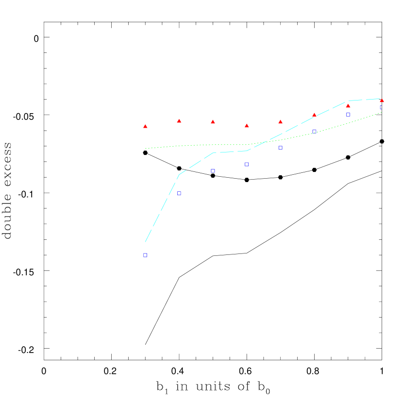
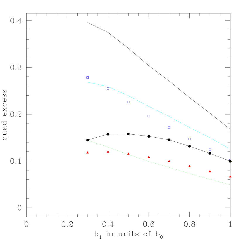
Figure 4: Contributions to doubles (left) and quads (right) from various effects. The lowest (uppermost) solid line is the full contribution. The filled triangles are the correlated contribution and the open squares are the uncorrelated contribution. The dotted and dashed lines are the contributions from within a radius of $5b_{0}$ and outside this radius respectively, and the filled hexagons with the line going through them show the contribution from the images associated solely to the primary. For images associated solely with the primary, the net total number of systems is lower, so to allow easier comparison with the other numbers, this curve has been rescaled to give the same net number of systems, thus giving the fractional contribution of these systems.

Figure 5: Comparison of SIS (with core) primaries and elliptical primaries. The fraction of doubles are shown on left, quads on right, plotted as a function of satellite mass. The solid line is the fraction of doubles or quads in the SIS (with core) case used for the bulk of the calculations, where the fractions found from an SIS primary and satellites are added to the fractions for an elliptical primary in isolation. The dashed lines are for elliptical primary lenses either aligned parallel or perpendicular to the direction of the satellite. The dotted line is the average of the two elliptical orientations. As the overlapping caustics of the two lenses was expected to cause the most variation from the ansatz used in the paper, separations only up to 5 $b_{0}$, five times the Einstein radius of the primary, were included; at and beyond this point the caustics of the two lenses are well separated. As can be seen in the plots the approximation used in the bulk of the calculations is quite close to the average of the two elliptical orientations for the quad case, for the double case the SIS calculation will actually tend to give an overestimate.

In our SIS+SIS model and the computation of the change in the quad fraction we model the number of two (four) image lenses produced by a more realistic SIE+SIS model as the sum of the number expected for an SIE in isolation with the excess cross section. We compare this simple model to results for the more realistic SIE+SIS models with satellites on either the major or minor axis of the lens in Figure 5. The results with the SIE bracket the SIS models with an average quite similar to our simpler spherical model. If we conducted a full suite of models at all inclinations we would simply fill in the region between the major and minor axis limits. We can crudely understand why ignoring the ellipticity of the primary lens has little effect on the result by considering a lens with two independent external shears $\gamma_{0}$ and $\gamma_{1}$ representing the ellipticity of the primary lens and the shear induced by a satellite respectively. The four-image cross section of the combined lens simply scales as $\gamma_{0}^{2}+\gamma_{1}^{2}+2\gamma_{0}\gamma_{1}\cos 2\Delta\Theta_{\gamma}$ where $\Delta\theta_{\gamma}$ is the angle between the two shear axes. The angle averaged cross section, $\sim\gamma_{0}^{2}+\gamma_{1}^{2}$, is simply the sum of the four-image cross section of the primary galaxy in isolation with that induced by the satellite on a spherical galaxy. Thus, while a complete calculation with elliptical primaries averaging over orientation is a logical next step, it should have little effect on our basic, quantitative conclusion. We also found that the non-circular models were 4–5 times more efficient at producing $n=5$ image systems.

True lenses will also have an external shear which can affect the quad to double ratio. We expect this shear to be random with respect to the elliptical axes of the primary and thus simulated random shears. Averaging over two shear orientations with ellipticity led to a net increase in the quad to double ratio, improving the effects of the satellite galaxies, just as would be expected from the argument above. A detailed study of the full parameter space would be interesting for future work.

3.1 Variations to Standard Model

Our standard model was based on treating close satellites of the primary lens as independent galaxies on larger scales. Using an empirical normalization for their abundance ($n_{*}$) helps keep the results from changing drastically under changes of the distribution of the satellites in mass or radius. To see how robust these results are, we consider here alternate assumptions about the distribution of the satellites in mass, separation and or internal structure.

We first consider changing from a Schechter distribution of satellites, motivated by galaxies, to a power law model motivated by CDM halo models. Simulations find halo mass functions that are power laws,

$${dn\over dM}=\frac{n_{*}}{M_{*}}\left({M\over M_{*}}\right)^{-1.8}$$ (24)

(e.g. Moore et al. Moo99 (1999), Klypin et al. Kly99 (1999)). with a normalization of $n_{*}=0.01h^{3}$ Mpc^-3 at $M_{*}=10^{12}h^{-1}M_{\odot}$ for a standard “concordance” model with $\sigma_{8}=0.9$ (Jenkins et al. Jen01 (2001)). If we are using a model with potentially dark halos, we should avoid normalizations based on the numbers of visible satellites. We convert mass to luminosity to critical radii (with distance dependence) as in section §2.

In the CDM picture, the number of low mass halos and galaxies rapidly diverges towards lower mass. NFW-like galaxy profiles (Navarro, Frenk & White NFW (1996), Moore et al. Moo99 (1999)) are expected when only gravitational forces are important, but these do not lens efficiently. Once baryonic cooling occurs, the halos contract to the very effectively lensing SIS profiles (e.g. Keeton Kee98 (1998), Porciani & Madau PorMad00 (2000), Kochanek & White KocWhi01 (2001), Li & Ostriker LiOst02a (2000, 2003)). In some sense, our Schechter function model for the satellites already is the correct model for the halos in which baryons have cooled. However, as an experiment, we also tried using the mass function of halos, cutting off the halos with such low circular velocities that they may have lost all their gas when the universe reionized (see Bullock, Kravtsov & Weinberg BulKraWei00 (2000)). We set this scale to $b_{1}=0.05b_{*}$ (corresponding to $v_{c}\simeq 50$ km/s), and then set the number of halos based on CDM simulations. Under these assumptions, we again find a significant suppression of the $n=2$ configurations, with $P_{e,2}/P_{tot}=-0.46$, a significant gain in the $n=4$ configurations, with $P_{e,4}/P_{tot}=1.12$, and a small contribution from non-standard configurations with $P_{e,3}/P_{tot}=0.12$ and $P_{e,5}/P_{tot}=0.05$. For these excess cross sections we would expect quads to significantly outnumber doubles with a 73:18 ratio, and again to have a small number of triples or quints.

We used an extrapolation of the correlation function, measured on large scales, to model the projected density of satellites in the inner regions of galaxies. In practice, large mass satellites which orbit too close to the center of the primary lens will undergo rapid orbital decay and be destroyed (e.g. Metcalf & Madau MetMad01 (2001)). This can be modeled by setting a scale $R_{fall}\sim 20$–$30$ kpc for the onset of the rapid decay, and then assuming there are no satellites interior to this radius. This leads to a modified correlation function $\xi_{2}(R)$ which flattens in the center to a constant value (roughly $\xi_{2}(R)\sim 10^{3}h^{-1}$ Mpc ) rather than continuing to rise as a power-law. However, since we must set the normalization $n_{*}$ to reproduce the observed numbers of satellites (finding $n_{*}=0.027\pm 0.009h^{3}$ Mpc^-3 for the $R_{fall}=22$ kpc case we tried as an experiment), the change in the radial structure has little effect on the lens statistics. Assuming the Schechter model for the satellite mass function, we find the now familiar suppression of the doubles, $P_{e,2}/P_{tot}=-0.16$, and enhancement of the quads, $P_{e,4}/P_{tot}=0.41$, leading (with the inclusion of the triples and fives) to an expectation of a quad:double ratio of 49:49 assuming lenses with a typical axis ratio of $f=0.7$, considering lenses associated with the primary alone gives a corresponding ratio of 35:62. Using the CDM inspired mass function instead of the Schechter model produces again significantly more quads, 67%, compared to 30% doubles.

As the correlation function at short distances is not well known, we also experimented with changing the logarithmic slope of $\xi(r)=(r/r_{0})^{-\gamma}$ from $\gamma=1.8$. For each case we estimated $n_{*}$ from the observed numbers of satellites. Steeper correlation functions weaken the effect of satellites. However, a steeper correlation function can also increase the number of quads significantly, if it is coupled with a restriction that no satellites occur within a fixed radius (such as 22 kpc). The cause of these correlations is easily understood from Fig. 1. For a fixed number of satellites, a steeper correlation function simultaneously adds weight to the central peak and reduces the weight of the resonance region, both of which will enhance the probability of producing two-image lenses. A shallower correlation function does the reverse, thereby enhancing the probability of producing four-image lenses. Better statistics for the distribution of lens galaxy satellites for different image morphologies may be able to discriminate between these models.

For our final experiment we truncated the halos of the two lenses by using pseudo-Jaffe models (Jaffe Jaf83 (1983), Keeton Kee01 (2001)) with $\rho\propto b(r^{2}+s^{2})^{-2}(r^{2}+a^{2})^{-2}$ and $a=10b$ rather than SIS models for the two lens components. Normalized by the total cross sections for the isolated pseudo-Jaffe models, the suppression of the doubles, $P_{e,2}/P_{tot}=-0.11$, and the enhancement of the quads, $P_{e,4}/P_{tot}=0.17$, is somewhat less than for our standard SIS+SIS models, raising the quad fraction from the 21% expected for $f=0.7$ ellipsoids to 35% rather than to 40%.

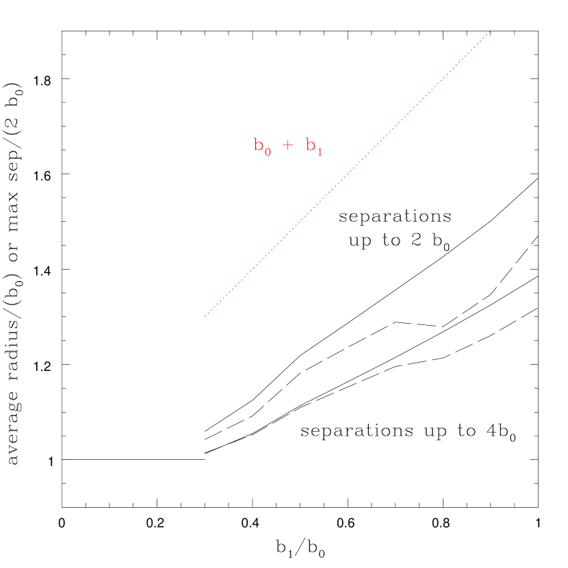
Figure 6: Biases in image separation estimates due to satellites. We show the average image radius (dashed line) and one-half the maximum image separation (solid line) in units of the critical radius of the primary lens $b_{0}$ as a function of the satellite critical radius $b_{1}$. We show the averages for regions with $R\leq 2b_{0}$ and $4b_{0}$.The dotted line shows the image critical radius $b_{0}+b_{1}$ which we would find if two SIS lenses are exactly aligned ($R=0$).

4 Conclusions

The high fraction of four-image lenses (50% of JVAS/CLASS lenses have four or more images) compared to the expectations for simple ellipsoidal lenses in reasonable tidal fields (20% to 30%) has been a long standing puzzle in understanding the statistics of gravitational lenses (King & Browne KinBro96 (1996), Kochanek 1996b , Keeton, Kochanek & Seljak kks (1997), Finch et al. Fin02 (2002), Rusin & Tegmark RusTeg01 (2001)). We find that the problem is largely explained by the changes in the caustic structures produced by including the effects of nearby satellite galaxies when we normalize the abundance of these satellites to match the abundance of satellites in the JVAS/CLASS lens sample. The satellites produce relatively small changes in the total lensing probabilities, but systematically suppress the probability of obtaining a two-image lens in favor of finding a four-image lens, with a small probability of finding non-standard 3 or 5 image lenses. Depending on the parameters and the assumptions, satellites can roughly double the 21% quad fraction expected for a typical elliptical galaxy (axis ratio $0.7$) up to a 35–50% quad fraction that is relatively easy to reconcile with the data. Provided we normalize the satellite abundance to the observations, this conclusion is little affected by the details of what we assume for the structure or spatial distribution of the satellites. A steeply rising mass function will have a notable effect, however, it is possible that the lowest mass satellites will be affected more strongly by tidal stripping and be less well approximated by the Faber-Jackson relation we assumed initially. It would be interesting to pursue this in a future work. The typical satellites responsible for the changes should have critical radii (luminosities) roughly 50% (25%) that of the primary lens, again consistent with the observations where the satellites in the JVAS/CLASS sample have luminosity ratios of $0.08$, $0.09$, $0.26$, $0.40$, $0.40$, $0.45$ relative to the primary lenses. The surveys should also find that $\sim$3% of the lenses should have non-standard multiplicities, which is borne out by the discovery of two higher multiplicity lenses (B1359+154, a 6 image lens produced by 3 galaxies in the CLASS survey, Myers et al. Mye99 (1999); and PMNJ0134–0931, a 5 image lens produced by 2 galaxies in the PMN survey, Gregg et al. Gre02 (2002), Winn et al. Win02 (2002)) in the flat-spectrum radio lens surveys.

The satellite galaxies can also interfere with efforts to estimate the cosmological model using lens statistics (e.g. Chae et al. Chaetal02 (2002), Davis, Huterer & Krauss Davis02 (2003) and references therein), as it is crucial in such studies to match the observed distributions of image separations in order to correctly estimate the lens cross sections (see Kochanek 1996a ). Close satellites modify the image separations, leading to biased estimates of the average multiple-imaging cross sections that in turn bias estimates of the cosmological model. Simply dropping lenses with satellites is not a solution because it builds a bias against high mass lenses into the calculation. The changes in the cross section produced by the satellite depend on the ratio $r=b_{1}/b_{0}$, while the luminosity of the satellite depends on $b_{1}^{2}=r^{2}b_{0}^{2}$. Thus, even though the satellites create the same fractional perturbation for all lenses, the satellites of the higher mass lenses are more easily detected simply because they are more luminous. For example, suppose every lens of luminosity $L_{0}$ had a satellite of luminosity $L_{1}=L_{0}/4$, and that we could detect any satellite with $L_{1}>L_{*}/4$. Every lens with $L_{0}>L_{*}$ would be rejected from the sample because it has a detectable satellite. The smaller average image separations of the final sample (only 68% that of the original sample) would lead to an underestimate of the average velocity dispersion (by about 20%) and cross section (by a factor of two) of the lenses. But the bias on the cross sections produced by the existence of satellites has not changed!All the lenses remaining in the sample have satellites producing the same fractional perturbations to the cross sections as they do in the rejected, massive systems. This is an extreme example, but the resulting bias in more realistic cases still represents a serious problem, and may explain the very low velocity dispersion scales found by Chae et al. (Chaetal02 (2002)) and Davis et al. (Davis02 (2003)).

Inclusion of the satellites does bias the image separations upwards, however, as shown in Fig. 6. We computed the average distance of the lensed images from the primary lens or one-half the maximum image separations, standard estimators for the average critical radius of a lens, as a function of the critical radius of the satellite. We included the weighting of the radial distribution of the satellites by the correlation function and computed the averages for the regions with $R\leq 2b_{0}$ and $4b_{0}$. The amplitude of the bias is modest except for systems with comparable masses. In particular, note that the average effect is significantly smaller than simply adding the critical radii of the two lenses. If we continue our (extreme) thought experiment of a sample of lenses all having satellites with $b_{1}/b_{0}=1/2$, we would overestimate the average image separations of an isolated lens by approximately 20% (using the $R<2b_{0}$ region, for a more detailed calculation one would choose this region self-consistently) if we simply used the observed image separations. For this case we would get an overestimate of the velocity dispersion (by about 10%) and the cross section (by 40%). However, the magnitude of the bias from simply including all the systems with satellites is only half that from excluding them.

In practice, the magnitude of the effect and the ambiguities arising from any simple treatment mean that reliable estimates of cosmological parameters or galaxy mass scales from lensing statistics cannot be based on isolated lenses. The calculations must include the effects of satellites. Fortunately, the model for the satellites, particularly the abundance of satellites, can be calibrated directly from the observations. As part of this process, more careful observational surveys need to be made of lens galaxy environments than the crude normalization estimates we made in §2.2. Alternatively the models can be checked against numerical simulations of lens environments (e.g. White et al. Whiteal01 (2001), Holder & Schechter HolSch02 (2003), Chen, Kravtsov & Keeton CheKraKee03 (2003)). Full calculations with elliptical lenses, large scale tidal shear fields and satellites should be done. We also limited our calculation to satellites, but more attention should be given to the statistical effects of embedding the lenses in more massive group or cluster halos. As the lens sample continues to grow, so does our ability to understand and quantitatively model the effects of satellites, so the ambiguities in statistical studies of lenses introduced by satellites will be resolved.

References

- (1) Bar-Kana, R., 1996, ApJ 468, 17
- (2) Blandford, R.D. & Kochanek, C.S., 1987, Ap. J, 321, 658
- (3) Blumenthal, G.R., et al, 1984, Nature, 341, 517
- (4) Blumenthal, G.r., Faber, S.M., Flores, R., Primack, J.R., 1986, ApJ, 301,27
- (5) Browne, I.W.A., Wilkinson, P.N., Patnaik, A.R., Wrobel, J.M., 1998, MNRAS 293, 257
- (6) Browne, I.W.A., et al., 2003, MNRAS 341, 13
- (7) Bullock, J.S., Kravtsov, A.V., Weinberg, D., 2000, ApJ 539, 517
- (8) Chae, K.-H., 2003, MNRAS 346, 746
- (9) Chae, K.-H., 2002, Phys.Rev.Lett. 89, 151301
- (10) Chen, J., Kravtsov, A.V., Keeton, C.R., 2003, ApJ 592,24
- (11) Chiba, M., 2002, ApJ 565, 17
- (12) Dalal, N., & Kochanek, C.S., 2002, ApJ 572, 25
- (13) Davis, A.N., Huterer, D., & Krauss, L.M., 2003, MNRAS 344, 1029
- (14) Evans, N.W., & Witt, H.J., 2003, MNRAS 345, 1351
- (15) Faber, S.M., & Jackson, R.E., 1976, ApJ 204,668
- (16) Finch, T.K., et al, 2002, ApJ 577, 51
- (17) Gregg, M., et al, 2002, ApJ 564, 133
- (18) Holder, G., Schechter, P., 2003, ApJ 589, 688
- (19) Jaffe, W., 1983, MNRAS, 202, 995
- (20) Jenkins, A., et al, 2001, MNRAS, 321, 372
- (21) Keeton, C.R., thesis.
- (22) Keeton, C.R., Kochanek, C.S. & Seljak, U., 1997,ApJ,483,604
- (23) Keeton, C.R., 2001, Catalogue of Lens Models, astro-ph/0102341
- (24) Keeton, C.R., 2003,ApJ 584, 664
- (25) Keeton, C.R., Gaudi, B.S., Petters, A.O., 2003, ApJ 598, 138
- (26) King, L.J., & Browne, I.W.A., 1996, MNRAS, 282,67
- (27) King, L.J., Browne, I.W.A., Marlow, D.R., Patnaik, A.R., Wilkinson, P.N., 1999, MNRAS 307, 225
- (28) Klypin, A., et al, 1999, ApJ, 522, 8
- (29) Kochanek, C.S., & Apostolakis, J., 1988, MNRAS 235, 1073
- (30) Kochanek, C.S., 1996, ApJ, 466, 638
- (31) Kochanek, C.S., 1996, ApJ, 473, 595
- (32) Kochanek, C.S., et al., 2001, ApJ 560, 566
- (33) Kochanek, C.S., White, M., 2001, ApJ 559, 531
- (34) Kochanek, C.S., Dalal, N., 2002, ApJ 572,25
- (35) Kochanek, C.S., Dalal, N., 2003, preprint [astro-ph/0302036]
- (36) Kovner, I. 1987, ApJ 316, 52
- (37) Li, L.-X., Ostriker, J.P., 2002, ApJ 566, 652
- (38) Li, L.-X., Ostriker, J.P., 2002, ApJ 595, 603
- (39) Loveday, J., 2000, MNRAS 512, 557
- (40) Mao, S., Schneider, P., 1998, MNRAS 295, 587
- (41) Metcalf, R. B., & Madau, P., 2001, ApJ 563, 9
- (42) Mo, H.J., Mao, S., White, S.D.M., 1998, MNRAS, 295,319
- (43) Moller, 0. & Blain, A.W., 2001, MNRAS 327, 339
- (44) Moore, B., et al., 1999, MNRAS, 310, 1147
- (45) Myers, S.T., et al., 1995, ApJ 447L, 5
- (46) Myers, S.T., et al., 1999, AJ 117, 2565
- (47) Myers, S.T., et al., 2003, MNRAS 341, 1
- (48) Navarro, J.F., Frenk, C.S., White, S.D.M., 1996, ApJ 462, 563
- (49) Patnaik, A.R., Browne, I.W.A., Wilkinson, P.N., & Wrobel, J.M., 1992, MNRAS 254, 655
- (50) Peacock, J.A., Cosmological Physics, (Cambridge University Press, 2001, Cambridge)
- (51) Porciani C., Madau, P. 2000, ApJ, 532, 679
- (52) Rees, M.J., Ostriker, J.P., 1977, MNRAS, 179, 541
- (53) Rusin, D., Tegmark, M., 2000, ApJ 553, 709
- (54) Rusin, D., et al., 2002, MNRAS 330, 205
- (55) Rusin, D., et al., ApJ 587, 143
- (56) Schechter, P., 1976, ApJ 203, 297
- (57) Schechter, P., Moore, C.B., 1993, AJ 105, 1
- (58) Schechter, P., Wambsganss, J., 2002, ApJ 580, 685
- (59) Seitz, S., Schneider, P., 1992, A & A, 265, 1
- (60) Silk, J., 1977, ApJ, 211, 638
- (61) Turner, E.L., Ostriker, J.P., Gott, J.R., 1984, ApJ, 284,1
- (62) White, S.D.M., Rees, M., 1978, MNRAS, 183,341
- (63) White, M., Hernquist, L, Springel, V, astro-ph/0107023
- (64) Wilkinson, P.N., Browne, I.W.A., Patnaik, A.R., Wrobel, J.M., Sorathia, B., 1998, MNRAS 300, 790
- (65) Winn, J., et al, 2002, ApJ 564, 143
- (66) Xanthopoulos et al, 1998, MNRAS 300, 649