Chandra Observations of the Central Region of Abell 3112

Abstract

We present the results of a Chandra observation of the central region of Abell 3112. This cluster has a powerful radio source in the center and was believed to have a strong cooling flow. The X-ray image shows that the intracluster medium (ICM) is distributed smoothly on large scales, but has significant deviations from a simple concentric elliptical isophotal model near the center. Regions of excess emission appear to surround two lobe-like radio-emitting regions. This structure probably indicates that hot X-ray gas and radio lobes are interacting. From an analysis of the X-ray spectra in annuli, we found clear evidence for a temperature decrease and abundance increase toward the center. The X-ray spectrum of the central region is consistent with a single-temperature thermal plasma model. The contribution of X-ray emission from a multiphase cooling flow component with gas cooling to very low temperatures locally is limited to less than 10% of the total emission. However, the whole cluster spectrum indicates that the ICM is cooling significantly as a whole, but in only a limited temperature range ($\geq 2$ keV). Inside the cooling radius, the conduction timescales based on the Spitzer conductivity are shorter than the cooling timescales. We detect an X-ray point source in the cluster center which is coincident with the optical nucleus of the central cD galaxy and the core of the associated radio source. The X-ray spectrum of the central point source can be fit by a 1.3 keV thermal plasma and a power-law component whose photon index is 1.9. The thermal component is probably plasma associated with the cD galaxy. We attribute the power-law component to the central AGN.

1 Introduction

The central regions of clusters of galaxies are very interesting and enigmatic places. The intracluster medium (ICM) in the central region is often so dense that its radiative cooling time is significantly shorter than the Hubble time. Therefore, the ICM will cool down unless it is heated significantly. Unbalanced radiative cooling would cause a “cooling flow” in the cluster center (see Fabian 1994 for a review). X-ray imaging analyses by ROSAT and EXOSAT indicated that mass deposition rates, $\dot{M}$, were more than $100\,M_{\odot}\,{\rm yr}^{-1}$ for many clusters (Edge, Stewart, & Fabian 1992; Allen & Fabian 1997; Peres et al. 1998). However, the fate of the resulting cold gas, or whether ICM in “cooling flow” clusters really cools down to low temperatures, is still unclear. The cD galaxies in cooling flows have an excess blue star component, which suggests that the cooled ICM forms new stars (McNamara & O’Connell 1989). However, the implied star formation rates are much lower than the cooling flow mass deposition ones (McNamara & O’Connell 1989). Furthermore, recent XMM-Newton high resolution spectroscopic observations have imposed a strong constraint on the amount of gas cooling down to low temperatures (Peterson et al. 2001; Kaastra et al. 2001; Tamura et al. 2001), which is consistent with the fact that the mass deposition rates determined spectroscopically by ASCA tended to be lower than those determined by EXOSAT and ROSAT (see Makishima et al. 2001 for a review).

The cD galaxies in the cooling flow clusters usually host strong radio sources, with a central radio core and/or radio lobes. Observations utilizing Chandra’s excellent spatial resolution have revealed interactions between these radio lobes and ICM, which may affect the dynamical and thermal history of ICM in the cluster center. In Hydra A (McNamara et al. 2000; David et al. 2001), Perseus (Fabian et al. 2000), and Abell 2052 (Blanton et al. 2001), radio lobes coincide with X-ray low surface brightness regions, which suggests that the radio plasma expands to displace the ICM. On the other hand, X-ray cavities without radio emission are also found at larger distances in Abell 2597 (McNamara et al. 2001). They are believed to be old radio lobes which cannot emit (at least at high radio frequencies) because the high energy relativistic electrons have already suffered radiative losses. These radio quiet cavities also indicate that cD galaxies provided the ICM with high energy electrons and magnetic fields intermittently.

Abell 3112 is a cooling flow cluster at a redshift of $z=0.0746$. There is a powerful radio source, PKS 0316-444, in the cluster center. Previous X-ray imaging analyses with EXOSAT (Edge, Stewart, & Fabian 1992) and ROSAT (Allen & Fabian 1997; Peres et al. 1998) indicated that Abell 3112 had a strong cooling flow, with a mass deposition rate of $\dot{M}\approx 400$ $M_{\odot}$ yr^-1. The temperature profile at a larger scale than the cooling radius was studied by Markevitch et al. (1998) and by Irwin, Bregman, & Evrard (1999) with ASCA data. Markevitch et al. (1998) found that the temperature decreased outward from 6 keV to 3 keV with ASCA data, although they explicitly assumed a cooling flow component in the central region. On the other hand, Irwin et al. (1999) argued that the data were consistent with an isothermal distribution. An increase in the iron abundance toward the center was reported by Finoguenov, David, & Ponman (2000). However, there was no detailed study of the temperature and abundance structure within the cooling radius ($\lesssim 250$ kpc) because of the limited spatial resolution of ASCA. Furthermore, any interaction region between the radio source and the ICM would be too small to have been resolved with ROSAT or ASCA. In this paper, we present Chandra observations of central region of Abell 3112. We assume $H_{0}=50$ km s^-1 Mpc^-1, $\Omega_{0}=1.0$, and $\Omega_{\Lambda}=0.0$. At a redshift $z=0.0746$, 1″ corresponds to 1.94 kpc. The errors correspond to the 90% confidence level throughout the paper.

2 Observations and Data Reduction

2.1 X-ray Observations

Abell 3112 was observed twice with Chandra on 2001 May 24 for 7,257 seconds and on 2001 September 15 for 17,496 seconds. Each observation was pointed so that the cluster center would fall near the aimpoint of the ACIS-S3 detector. However, the roll angles were different, so the outer parts of the field of view differ for the two observations. The two observations were merged, using the positions of bright point sources to register the two images. Here, we analyze data from the S3 chip only. The data from the S1 chip was used to search for the background flares. A few short periods with background flares were found and removed using the lc_clean software provided by Maxim Markevitch, leaving a total exposure of 21,723 seconds. Only events with ASCA grades of 0, 2, 3, 4, and 6 were included. Standard bad pixels and columns were removed. Exposure maps and background data were generated for each observation separately, and then merged appropriately. Blank sky background data were taken from the compilation by Maxim Markevitch.

The data are possibly affected by the low energy QE degradation of ACIS. We tried to correct this using the corrarf program. However, the correction did not appear to work well for this data; specifically, corrarf seemed to over-correct the data. As a result, we obtained absorption column densities which were much lower than the Galactic value in our spectral fits. We expect that the absorbing column should be at least as large as the Galactic value. Therefore, we will show the results without the correction for the low energy QE degradation. Fortunately, this correction significantly affects only the very low energy ($\leq$ 1 keV) part of the Chandra band. As a result, neither temperature nor abundance determinations were seriously affected by this correction. On the other hand, mass deposition rates of cooling flow components increased by a factor of about two when we fitted the spectra after the correction.

2.2 Radio observations

The observations were made with Very Large Array at a center frequency of 1320 MHz on 1996 October 18. The array was in the ‘A’ configuration, which provided an angular resolution of 6.9 $\times$ 1.5 arcsec. A total of 1.2 hours were obtained on source using 32 channels across a 6.25 MHz band. Both right and left circular polarizations were observed. Phase and bandpass calibration was obtained by short (1 min) observations of the strong (4.9 Jy) calibrator J0440-4333 taken every $\sim$20 minutes. Atomic hydrogen absorption was searched for towards the compact core over a velocity range from 22,100–23,440 km s^-1 at a resolution of 44 km s^-1, but not detected down to a 3$\sigma$ limit on the maximum optical depth of 0.012.

3 X-ray Images

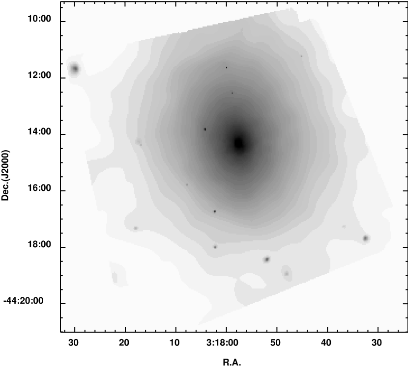
Figure 1: Adaptively smoothed Chandra image (0.3-10.0 keV) with a minimum signal-to-noise of 3 per smoothing beam. The image has been background subtracted and corrected for exposure and vignetting.

The X-ray image was adaptively smoothed using the ciao csmooth program with a minimum signal-to-noise of 3 per smoothing beam. An identically-smoothed background was subtracted, and the image was divided by an identically-smoothed exposure map. The exposure map was corrected for vignetting, using the typical energy of the observed photons to take account of the energy dependence of the vignetting. The resulting image is shown in Figure 1. As in other typical cooling flow clusters, X-ray emission is distributed symmetrically and is fairly concentrated in the center. The image is smooth and quite symmetric on large scales. The cluster emission is elliptical, with a major axis along the direction from NNE to SSW. On large scales, there appears to be no substructure except for some point sources.

We used a wavelet detection algorithm (WAVEDETECT in CIAO) to detect individual point sources. Sources were visually confirmed on the X-ray image, and a few low-level detections were removed. Using this method, we found sixteen point sources. One of these corresponds to the radio source PKS 0316-444, which is located at the center of the central cD galaxy ESO 248- G 006. Another corresponds to a galaxy in the cluster (LCRS B031619.9-442441).

The regularity of the cluster X-ray emission on large scales doesn’t continue into the very central region. Figure 2 shows the X-ray contour map of the $\sim 1^{\prime}\times 1^{\prime}$ region around the central point source. In the very center, an elongated structure from the central point source towards the SE is clearly seen. We can see another filament-like component from $\sim 10\arcsec$ south of the central point source towards the SW. To clarify structures which deviate from symmetric cluster emission, we fitted the entire cluster image with a concentric elliptical isophotal model, and then subtracted the best-fit model from the image to get the residual component. In the fitting procedure, we fixed the center of the isophotes to the center determined from the larger scale isophotes about which the image was symmetric, rather than the central point source. The ellipticity and position angle for each isophote were allowed to vary. It is most likely that relaxed cluster potential structure is not spheroidal but triaxial (Jing & Suto 2001). In this case, the ICM hydrostatic density distribution also will be triaxial (Lee & Suto 2003). Therefore, the ellipticities and the position angles of X-ray isophotes can vary with radius unless our line-of-sight coincides with one of the three symmetry axes.

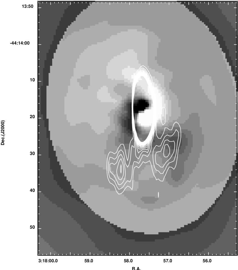
Figure 3: The greyscale shows the residuals of the adaptively-smoothed X-ray image (0.3–10 keV) from our best-fit elliptical isophotal model. Dark areas are positive residuals (excess emission), while light areas are negative residuals. The dark and light regions at the center are due to the central point source, which is not exactly at the center of the X-ray isophotes at large radii. The contours are from the 1.32 GHz VLA radio image. The very bright radio core is coincident with the central X-ray source. The NS extension of the radio core source is due to the elongated radio observing beam.

In Figure 3, the greyscale shows the residual produced by subtracting our best-fit elliptical isophotal model from the adaptively smoothed image of the central region of the cluster. The sharp elliptical edge near the outside is an artifact because the elliptical model extended only to this isophote. Dark areas are positive residuals (excess emission), while light areas are negative residuals. The dark and light regions at the center are due to the central point source, which is not exactly at the center of the X-ray isophotes at large radii. There are regions of excess emission to the south of the central source. The contours show the 1.32 GHz VLA radio image. There is a very bright radio core, which is unresolved in the radio image; the elliptical contours for the core show the beam of the radio observation. The very bright radio core is coincident with the central X-ray source. There are two diffuse radio regions to the SE and SW of the radio core, which may be connected to the core. The NS extent of these regions is presumably exaggerated due to the elongated observing beam. Roughly speaking, the excess X-ray regions appear to surround two lobe-like radio components. However, part of the SW radio lobe is coincident with a region of X-ray excess emission. Unfortunately, the low resolution of the radio data, bright radio core, and elongated radio beam make it difficult to decide definitely whether the excess is in the radio lobes or partly surrounding it.

4 Spectral Analysis

In order to examine the temperature and abundance structure quantitatively, we determined the X-ray spectra in annuli. We fitted the data between 0.5 and 10.0 keV with a photo-absorbed single temperature MEKAL model (Kaastra 1992; Liedahl, Osterheld, & Goldstein 1995) after masking the point sources. We tried to fit the data fixing the absorbing column density to the Galactic value ($N_{H}=2.51\times 10^{20}$ cm^-2; Dickey & Lockman 1990) or allowing it to vary freely. The fitting results depend somewhat on whether we fixed the absorption to the Galactic value or not. Figure 4 shows the radial temperature and abundance profiles. The solid crosses are the values obtained when we allowed the absorption to vary, while the dashed crosses are the values when we fixed the absorption to the Galactic value. The dashed crosses are shifted slightly to the left in order to be more easily seen. The results with fixed or varying absorption are similar. At $r>70\arcsec$, both the temperature and abundance are nearly constant at $kT\sim 6$ keV and $Z\sim 0.4\,Z_{\odot}$, respectively. The temperature decreases from $\sim 6$ keV at 70″ to 3.5 keV in the central 20″. The abundance increases from $\sim 0.4\,Z_{\odot}$ at 70″ to 1.3 $Z_{\odot}$ in the central 20″.

The temperature values obtained with variable absorption, along with their associated errors, are fitted to a power-law profile given by $T(r)=T_{0}(r/1\arcsec)^{p}$. For $r<70\arcsec$, $T_{0}=1.838\pm 0.254$ keV and $p=0.270\pm 0.044$. For $r>70\arcsec$, $T_{0}=4.226\pm 3.174$ keV and $p=0.064\pm 0.165$. We will use these fitted temperature profiles later when we analyze conduction timescale and integrated gravitational mass.

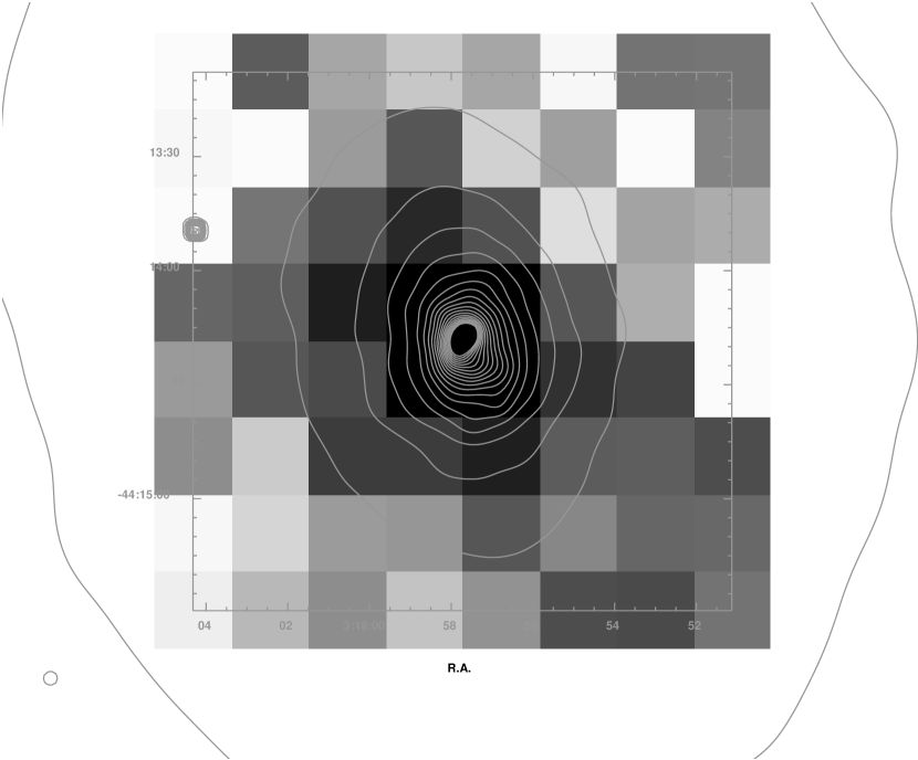
Figure 5: A two-dimensional temperature map of the central $240\arcsec\times 240\arcsec$ region overlaid with X-ray surface brightness contours. Black and white represent lower ($\sim 3keV$) and higher ($\sim 6keV$) temperature, respectively.

To examine the non-radial temperature structure, we made a two-dimensional temperature map of the central $240\arcsec\times 240\arcsec$ region. We divided the region into 64 ($8\times 8$) square regions, each of which is $30\arcsec\times 30\arcsec$. Then, we fitted the data of each region with the photo-absorbed MEKAL model where absorption is treated as a free parameter. Figure 5 shows a two-dimensional temperature map of the central $240\arcsec\times 240\arcsec$ region overlaid with X-ray surface brightness contours. Black and white represent lower ($\sim 3$ keV) and higher ($\sim 6$ keV) temperatures, respectively. There is no significant azimuthal structure in the temperature map while temperature decrease toward the center is again clearly seen. We also made a two-dimensional abundance map in the same way. However, abundances in the individual fits were too poorly constrained to provide a useful map.

We tried to fit the annular spectra with a model for a multiphase cooling flow to constrain the contribution from a cooling flow component and a mass deposition rate in each annulus, although the data within each annulus are almost consistent with a single temperature MEKAL model. As a cooling flow spectral model, we used the MKCFLOW model based on the MEKAL model. We added a MEKAL model representing the emission from the ICM outside the cooling flow. Both MKCFLOW and MEKAL were assumed to be subject to the same absorption column, which we fixed to the Galactic value or let vary freely. We fixed the metallicity and initial gas temperature of the MKCFLOW model to the same values of metallicity and temperature as the MEKAL model, respectively. The low temperature in the MKCFLOW model is fixed to the lowest value (0.001 keV) in XSPEC. The results are shown in Table 1 and 2. Compared with the fitting results without cooling flows, the results are not improved dramatically. Figure 6 shows a radial profile of the mass deposition rate derived from the fitting. The circles and solid error bars are the values obtained from fits with freely varying absorption. The squares and dashed error bars are the values from the fits with fixed Galactic absorption. When absorption is set as a free parameter, forth bin and the outermost three bins are consistent with a model without a cooling flow component. Only the inner three bins and the fifth bin have the cooling flow component, although their errors are fairly large and comparable to themselves. The resultant total mass deposition rate is $44.5^{+52.1}_{-32.5}\,M_{\odot}$ yr^-1, which is significantly smaller than the rates derived from the previous image analyses of EXOSAT and ROSAT data, which are $\sim 400\,M_{\odot}$ yr^-1 (Edge, Stewart, & Fabian 1992; Allen & Fabian 1997; Peres, et al. 1998). The cooling flow component contributes less than $\sim 10$% of the total X-ray emission. When we adopt the Galactic absorption value, the mass deposition rate becomes even lower and consistent with a model without a cooling flow component in all bins.

Even though multiphase gas is not found within small regions of the cluster, we do see an overall temperature gradient, with gas in the center that is cooler by a factor of $\sim 2$ compared with gas in the outer regions of the cluster. Therefore, if we fit a spectrum extracted from the whole cluster, a significant mass deposition rate and a low temperature cutoff might be expected. We fit the data within $157\arcsec$ with the MEKAL plus MKCFLOW model where the low temperature in MKCFLOW is allowed to vary. The results are shown in Table 3. The upper and lower rows show the results with the absorption column allowed to vary and fixed to the Galactic value, respectively. In contrast to the spectral analyses in annuli, the mass deposition rate is comparable with the former values based on imaging analysis. However, the low temperature in the MKCFLOW model is not very low ($kT_{\rm Low}\sim 2$ keV), which means that the observations are consistent with significant cooling, but only over a limited temperature range. This is consistent with what has been observed with many cooling flow clusters using Chandra and XMM-Newton (e.g., Peterson et al. 2003). Please note that the goodness of the fit is marginal (the reduced chi-squared is about 1.5). This might indicate that the emission measure distribution with the temperature is not that of the standard cooling flow model even in the temperature range between $T_{\rm High}$ and $T_{\rm Low}$.

5 X-ray Profiles and Deprojection

To quantify the radial structure of the ICM, we made a radial profile of the X-ray surface brightness in the 0.3-10.0 keV band (Figure 7a). The bins for X-ray surface brightness were chosen to be the same as those used below to determine the radial variation in the X-ray spectrum (§ 4). The surface brightness values were deprojected to determine the X-ray emissivity and gas density (Figure 7b), assuming the emissivity is constant in spherical shells. When we convert the emissivity into the gas density, we use a MEKAL code and assume that the temperature is constant in spherical shells and equal to that derived from the spectral fitting of projected data. Some fluctuations are seen in the density and pressure profiles near the outer boundary (Figure 7b and 7c), which are artifacts of the deprojection since we assume zero emissivity outside the outer boundary. However, many simulations of our deprojection method show that this affects only a few outermost points, and has no significant effect anywhere near the center. The observed gas density and pressure profiles are quite smooth outside of the region of the radio source. Based on the smooth radial profiles and lack of substructure in the X-ray image outside of the radio source region, we conclude that this cluster is dynamically relaxed and that the ICM is generally in hydrostatic equilibrium.

6 Mass Distributions

The gravitational mass distribution was determined from the equation of hydrostatic equilibrium,

$$M_{\rm tot}(<r)=-\frac{k_{B}Tr}{\mu m_{p}G}\biggl{(}\frac{d\ln\rho_{\rm gas}}{d\ln r}+\frac{d\ln T}{d\ln r}\biggr{)}.$$ (1)

We use the fitted power-law temperature profiles when $M_{\rm tot}(r)$ is calculated. To reduce the noise in the density gradient term, we determine the gradient at $r_{i}$ by differencing the densities at $r_{i-2}$ and $r_{i+2}$. Uncertainties in the density gradient at $r_{i}$ are also calculated from the density uncertainties at $r_{i-2}$ and $r_{i+2}$. The density gradients and their uncertainties are assumed to be equal in the innermost three points and the outermost three points. The gas mass profile is also determined from the ICM density profile assuming spherical symmetry. The gas mass is then given by

$$M_{\rm gas}(<r)=\int^{r}_{0}\rho_{gas}(r)4\pi r^{2}dr$$ (2)

The integrated gravitational mass and gas mass are shown in Figure 8 (a).

A radial profile of the gas mass fraction is shown in Figure 8 (b). The gas mass fraction increases from $3\%$ at $10\arcsec$ to $10\%$ at $100\arcsec$. This trend is similar to those in other well-relaxed clusters (David, Jones, & Forman 1995; Ettori, & Fabian 1999; Allen, Schmidt, & Fabian 2002). Our gas mass fraction is lower than that of Mohr, Mathiesen, & Evrard (1999) at much larger radii ($>$ 1 Mpc), but the gas fractions of clusters generally increase with radius, and this appears to apply to Abell 3112. Using the same beta-model fits as in Mohr et al., we find that the gas fraction at $100\arcsec$ is predicted to be $\sim$12%, which agrees well with our values.

7 Comparison of Cooling and Thermal Conduction

Because the temperature is higher than $\sim 3$ keV over the whole cluster, the main emission mechanism is thermal bremsstrahlung. Therefore, the isobaric cooling time is (Sarazin 1986)

$$t_{\rm cool}=8.5\times 10^{10}\biggl{(}\frac{n_{p}}{10^{-3}\,{\rm cm}^{-3}}\biggr{)}^{-1}\biggl{(}\frac{T}{10^{8}\,{\rm K}}\biggl{)}^{1/2}\,{\rm yr}$$ (3)

Radiative cooling would make a radial temperature gradient in the central region of the ICM through its density dependence, as is observed. (Fig. 4). On the other hand, thermal conduction would have the effect of reducing the temperature gradient. The conduction timescale is generally expressed as (see also Sarazin 1986)

$$t_{\rm cond}=\frac{n_{e}l_{T}^{2}k_{B}}{\kappa}$$ (4)

where $n_{e}$ is electron number density, $l_{T}=T/\nabla T$ is the scale length of the temperature gradient, and $k_{B}$ is the Boltzmann constant. If we consider only the Coulomb scattering process, the thermal conductivity for hydrogen plasma is (Spitzer 1962)

$$\kappa=4.6\times 10^{13}\biggl{(}\frac{T_{e}}{10^{8}\,{\rm K}}\biggr{)}^{-5/2}\biggl{(}\frac{\ln\Lambda}{40}\biggr{)}^{-1}\,{\rm erg}^{-1}\,{\rm cm}^{-1}\,{\rm K}^{-1}\,,$$ (5)

where $\ln\Lambda$, the Coulomb logarithm, is

$$\ln\Lambda=37.8+\ln\biggl{[}\biggl{(}\frac{T_{e}}{10^{8}\,{\rm K}}\biggr{)}\biggl{(}\frac{n_{e}}{10^{-3}\,{\rm cm}^{-3}}\biggr{)}^{-1/2}\biggr{]}.$$ (6)

Figure 9 shows radial profiles of $t_{\rm cool}$ and $t_{\rm cond}$. When we calculated $t_{\rm cond}$, we used the fitted power-law temperature profile to reduce the noise in the temperature gradient. Also, $t_{\rm cond}$ is evaluated only for $r<70\arcsec$ because an isothermal distribution is consistent with the temperature data in the outer regions.

The cooling time of the innermost bin is $2\times 10^{9}$ yr. If we define a cooling radius as where $t_{\rm cool}$ is $1.5\times 10^{10}$ yr, it becomes $\sim 100\arcsec$, or $\sim 200$ kpc. Both results are consistent with the former ROSAT (Allen & Fabian 1997; Peres et al. 1998) and EXOSAT results (Edge, Stewart, & Fabian 1992). At the innermost three bins, $t_{\rm cool}$ and $t_{\rm cond}$ are comparable with each other. Outside of this region, the conduction timescale is clearly shorter than the cooling timescale. If conduction proceeded at the Spitzer rate, it would erase the temperature gradient. Since the observations show a significant gradient in this region (Fig. 4a), thermal conduction must be significantly suppressed by, e.g., tangled magnetic fields and/or plasma instabilities. The cooling rate of gas with solar abundance is only $\sim$ 10% higher than that of hydrogen-helium mixture gas at 3.5 keV (see Figure 9-9 of Binney & Tremaine 1987). Therefore, actual cooling timescales in the central regions are probably $\sim$ 10% shorter at the most, which does not change the situation here dramatically. Although our estimation here is rough, it is still useful for an estimation of an order of magnitude. Calculations taking account of time evolution will be helpful to make more precise models.

8 The Central Point Source

We detected an X-ray point source in the cluster center. The position is coincident with the optical core of the cD galaxy and the radio core. The position of the X-ray point source is (epoch J2000) $\alpha=03^{h}17^{m}57.65^{s}$ $\delta=-44^{\circ}14\arcmin 17.06\arcsec$ with an uncertainty of 0.04 arcsec in each coordinate. The spectrum of the point source is shown in Figure 10. We fitted the data with a MEKAL model plus a power-law model. In addition to the absorption column density common for both components, we added intrinsic absorption for the power-law component only. As a result, the applied model is

$${\rm Model}_{\rm AGN}={\rm WABS}\times[{\rm MEKAL}+{\rm ZABS}\times{\rm POWERLAW}].$$ (7)

The abundance of the MEKAL component was fixed to the value derived from the region surrounding the point source. The absorbing column $N_{\rm H}$ was also fixed either to the value derived from the surrounding region or the Galactic value. The fitting results are shown in Table 4. The spectral model consists of a 1.26 keV thermal plasma component and a power-law component with a photon index of $\sim 1.9$. The power-law component has an extra absorbing column of $\sim 2\times 10^{21}$ cm^-2. This is consistent with the central source being a strongly absorbed AGN.

9 Discussion

We found that the central radio source associated with the central cD galaxy in Abell 3112 is interacting with the surrounding ICM (Fig. 2 and 3). The radio image shows a central core and two diffuse lobes to the SE and SW of the core. The central X-ray image has an asymmetric structure, and the excess X-ray emission over an elliptical isophotal model roughly appears to surround two radio lobes. This configuration is naturally explained if the radio lobes have swept up the ICM which was where the radio lobes are now. Similar scenarios have been proposed in other cooling flow clusters with radio sources (e.g., McNamara et al. 2000; Fabian et al. 2000; Blanton et al. 2001 ). In addition, there is excess X-ray emission coincident with part of the SW radio lobe. It is possible that the excess X-ray emission is due to the cool gas that was originally near the very center; this cool gas might have been entrained by hot buoyant bubbles. This scenario was originally proposed to explain the X-ray morphology of the central region of M87 (Churazov et al. 2001). Indeed, the filamentary structures in the X-ray image of the central region of Abell 3112 (Figure 2) are similar to those in M87 (Feigelson et al. 1987; Böhringer et al. 1995). This model may also apply to Abell 133 (Fujita et al. 2002). In order to determine which model applies to Abell 3112, temperature and abundance measurements of the excess X-ray components would be useful because the excess components are expected to have higher abundances and lower entropy in the entrainment scenario. Unfortunately, the present data have too few counts in these regions to allow a detailed spectral analysis. A deeper radio image would also be useful, as would lower frequency observations to search for steep spectrum emission. Note that the effect of the central radio source is limited to a region very close ($r\sim 10\arcsec$) to the center. This region is much smaller than the cooling flow region itself ($r\sim 100\arcsec$). Outside the interacting region, there is no evidence of the interaction such as X-ray cavities, instead the X-ray image is quite symmetric and smooth. Therefore, the central radio source does not directly affect the structure of the cooling flow outside of the very central region, at least at present. Note that we only have high frequency radio data. Low frequency radio observations might give another picture. In the case of M87 in the Virgo cluster, for instance, 327 MHz radio data show an morphology which fills out a large portion of the central region of the cluster (Owen, Eilek, & Kassim 2000), although similar structures cannot be seen in higher frequency data.

Radiative cooling produces a temperature decrease towards the center of the cluster. On the other hand, thermal conduction would reduce this temperature gradient. If we adopt the standard Spitzer conductivity, conduction would be expected to be very effective and to have eliminated the central temperature gradient (Figure 9). However, the observations show that the temperature does decrease significantly at the center of the cluster. This implies that thermal conduction is significantly suppressed below the Spitzer value.

Although we did not find a large amount of locally cooling multiphase gas, the existence of a large-scale temperature gradient indicates that the ICM is cooling in a global scale. The mass deposition rate of Abell 3112 determined from our spectroscopy of the total spectrum is comparable to that determined previously based on ROSAT and EXOSAT image analyses (Edge, Stewart, & Fabian 1992; Allen & Fabian 1997; Peres et al. 1998). However, the temperature range of the cooled gas is limited to $\geq 2$ keV. In addition, emission measure distribution about temperature is probably different than that expected from the standard cooling flow model. This suggests that some other heating mechanism may affect the cooling gas. One probable solution is heat conduction which is reduced from the Spitzer value by some physical mechanism but still is energetically important (e.g., Hattori & Umetsu 2000; Malyshkin & Kulsrud 2001). The relativistic electrons from the central radio source might also supply the required heating (e.g., Fabian et al. 2000; McNamara et al. 2000; David et al. 2001; Blanton et al. 2001). However, it is unlikely that the radio-emitting electrons are heating all of the cooling gas in Abell 3112 at present, because the radio lobes are so small that they do not directly affect the cooling flow on large scales. In Abell 3112, there is no evidence for ghost bubbles which might indicate a history of past radio source interactions (McNamara et al. 2001). Another possible form of radio source heating would be high energy protons from the central AGN. Since the minimum energy density in relativistic electrons is too small to support radio bubbles against the surrounding hot gas (e.g., Blanton et al. 2001), most of the energy in the radio source may be in the form of relativistic protons. The accelerated protons could diffuse and heat the ICM through Coulomb interactions (Rephaeli & Silk 1995; Inoue & Sasaki 2001). Although they do not emit any observable radio radiation, protons would produce several hundred MeV $\gamma$-rays through the decay of neutral pions produced in collisions with thermal protons. Future $\gamma$-ray observations will test this hypothesis.

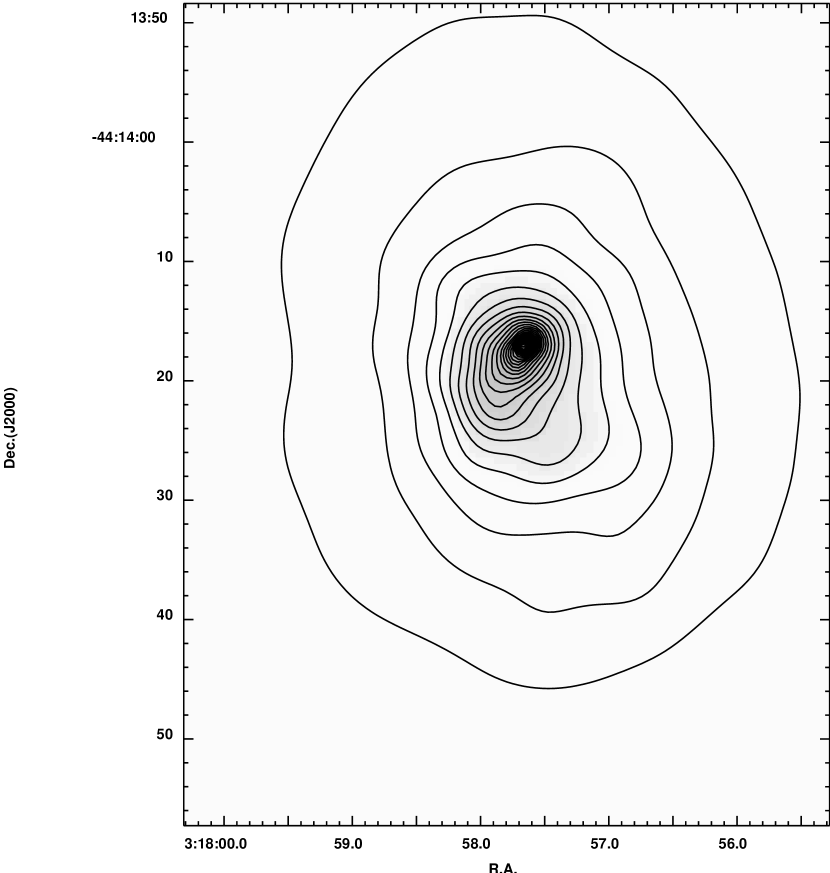
Figure 2: X-ray contour map (0.3-10.0 keV) of the central $\sim 50\arcsec\times 70\arcsec$ region of the cluster Abell 3112. Contours are logarithmically spaced. In the very center, an elongated structure is seen extending from the central point source towards the SE. Another filament extends from $\sim 10\arcsec$ south of the central point source towards the SW.

Figure 4: Radial profiles of temperature (a) and abundance (b), respectively. The solid crosses are the values obtained when we allowed the absorption to vary, while the dashed crosses are the values when we fixed the absorption to the Galactic value.

Figure 6: Radial profile of the mass deposition rate. The circles and solid error bars are the values obtained when we allowed the absorption to vary, while the squares dashed error bars are the values when we fixed the absorption to the Galactic value.

Figure 7: Radial profiles of surface brightness (a), electron density (b), and pressure (c), respectively.

Figure 8: (a) Integrated total gravitational mass (diamonds) and gas mass (triangles). (b) Radial profile of gas mass fraction. The gas mass fraction increases from $3\%$ at $10\arcsec$ up to $10\%$ at $100\arcsec$.

Figure 9: Radial profiles of isobaric cooling timescales (circles) and thermal conduction timescales (squares). At the innermost three bins, cooling and conduction timescales are comparable with each other. Outside this region, conduction timescales are clearly shorter than cooling timescales.

Figure 10: Spectrum of the central point source. The spectrum is fit by a 1.26 keV thermal plasma plus a power-law component whose photon index is 1.9. The power-law component has an intrinsic extra absorption column of $\sim 2\times 10^{21}$ cm^-2. This is consistent with the central source being a strongly absorbed AGN.

Table 1: Cooling Flow Spectra in Each Annulus with Variable Absorption

$r$	$kT_{\rm High}$	$Z$	$N_{\rm H}$	$\dot{M}$	$\chi^{2}/{\rm dof}$
(arcsec)	(keV)	($Z_{\odot}$)	($10^{20}$ cm-2)	($M_{\odot}$ yr-1)
$0-20$	$3.58^{+0.16}_{-0.14}$	$1.16^{+0.16}_{-0.14}$	$5.20^{+0.86}_{-0.82}$	$13.59^{+8.32}_{-8.09}$	284.5/200
$20-39$	$4.65^{+0.47}_{-0.22}$	$0.79^{+0.15}_{-0.11}$	$4.42^{+0.80}_{-0.76}$	$8.68^{+7.14}_{-8.40}$	285.3/233
$39-59$	$5.60^{+0.61}_{-0.45}$	$0.55^{+0.13}_{-0.12}$	$4.26^{+0.93}_{-0.89}$	$13.82^{+8.67}_{-8.34}$	226.2/216
$59-79$	$5.70^{+0.69}_{-0.39}$	$0.45^{+0.14}_{-0.12}$	$3.36^{+1.00}_{-0.86}$	$0.00^{+7.31}_{-0.00}$	234.3/205
$79-98$	$5.74^{+0.90}_{-0.63}$	$0.38^{+0.15}_{-0.14}$	$4.32^{+1.21}_{-1.13}$	$8.37^{+7.59}_{-7.52}$	222.9/195
$98-118$	$5.69^{+0.71}_{-0.50}$	$0.40^{+0.16}_{-0.16}$	$3.11^{+1.16}_{-1.04}$	$0.00^{+4.68}_{-0.00}$	216.8/188
$118-138$	$6.22^{+0.86}_{-0.66}$	$0.50^{+0.23}_{-0.21}$	$2.65^{+0.63}_{-1.14}$	$0.00^{+2.95}_{-0.00}$	202.5/181
$138-157$	$5.70^{+1.36}_{-0.65}$	$0.47^{+0.24}_{-0.21}$	$3.49^{+1.64}_{-1.40}$	$0.15^{+5.41}_{-0.15}$	204.5/175

Table 2: Cooling Flow Spectra in Each Annulus with Fixed Absorption

$r$	$kT_{\rm High}$	$Z$	$N_{\rm H}$	$\dot{M}$	$\chi^{2}/{\rm dof}$
(arcsec)	(keV)	($Z_{\odot}$)	($10^{20}$ cm-2)	($M_{\odot}$ yr-1)
$0-20$	$3.63^{+0.24}_{-0.11}$	$1.27^{+0.16}_{-0.14}$	($2.51$)	$0.55^{+7.39}_{-0.55}$	315.6/201
$20-39$	$4.87^{+0.32}_{-0.24}$	$0.88^{+0.13}_{-0.12}$	($2.51$)	$0.80^{+6.64}_{-0.80}$	302.5/234
$39-59$	$5.65^{+0.64}_{-0.42}$	$0.60^{+0.13}_{-0.12}$	($2.51$)	$5.32^{+6.529}_{-5.32}$	237.1/217
$59-79$	$5.92^{+0.63}_{-0.31}$	$0.46^{+0.15}_{-0.12}$	($2.51$)	$0.00^{+4.13}_{-0.00}$	236.9/206
$79-98$	$5.81^{+0.92}_{-0.50}$	$0.43^{+0.15}_{-0.14}$	($2.51$)	$2.20^{+6.06}_{-2.20}$	230.1/196
$98-118$	$5.84^{+0.67}_{-0.39}$	$0.41^{+0.17}_{-0.15}$	($2.51$)	$0.00^{+3.08}_{-0.00}$	217.7/189
$118-138$	$6.26^{+0.80}_{-0.54}$	$0.49^{+0.25}_{-0.18}$	($2.51$)	$0.00^{+2.56}_{-0.00}$	202.5/182
$138-157$	$5.94^{+1.25}_{-0.50}$	$0.50^{+0.26}_{-0.21}$	($2.51$)	$0.00^{+3.44}_{-0.00}$	205.85/176

Table 3: Total Spectrum ($r<157\arcsec$)

$kT_{\rm High}$	$kT_{\rm Low}$	$Z$	$N_{\rm H}$	$\dot{M}$	$\chi^{2}/{\rm dof}$
(keV)	(keV)	($Z_{\odot}$)	($10^{20}$ cm-2)	($M_{\odot}$ yr-1)
$7.42^{+0.12}_{-0.84}$	$1.86^{+0.46}_{-0.22}$	$0.58^{+0.05}_{-0.05}$	$4.01^{+0.32}_{-0.31}$	$609^{+51}_{-133}$	$699.0/474$
$9.07^{+0.50}_{-1.52}$	$2.02^{+0.31}_{-0.23}$	$0.68^{+0.06}_{-0.05}$	$(2.51)$	$544^{+34}_{-67}$	$758.7/475$

Note. – The upper and lower rows show the results with absorption column density allowed to vary and fixed to the Galactic value, respectively.

Table 4: Spectrum of the Central Point Source

$kT$	$Z$	$N_{\rm H}$	$\Gamma$	$\Delta N_{\rm H}$	$\chi^{2}/{\rm dof}$
(keV)	($Z_{\odot}$)	($10^{20}$ cm-2)		($10^{20}$ cm-2)
$1.26^{+0.15}_{-0.17}$	$(0.77)$	$(6.40)$	$1.89^{+0.30}_{-0.38}$	$18.8^{+18.1}_{13.6}$	12.9/21
$1.26^{+0.14}_{-0.17}$	$(1.27)$	$(2.51)$	$2.00^{+0.26}_{-0.18}$	$25.3^{+14.8}_{11.4}$	12.9/21

Note. – The abundance and $N_{\rm H}$ of the MEKAL component were derived from the fit of the region surrounding the point source. Upper and lower rows show the results when the $N_{\rm H}$ is allowed to vary or fixed to the Galactic value, respectively.

References

- (1) Allen, S. W., & Fabian, A. C. 1997, MNRAS, 286, 583
- (2) Allen, S. W., Schmidt, R. W., & Fabian, A. C. 2002, MNRAS, 334, L11
- (3) Binney, J., & Tremaine, S. 1987, Galactic Dynamics (Princeton: Princeton Univ. Press)
- (4) Blanton, E. L., Sarazin, C. L., McNamara, B. R., & Wise, M. W. 2001, ApJ, 558, L15
- (5) Böhringer, H., Nulsen, P. E. J., Braun, R., & Fabian, A. C. 1995, MNRAS, 274, L67
- (6) Churazov, E., Brüggen, M., Kaiser, C. R., Böhringer, H., & Forman, W. 2001, ApJ, 554, 261
- (7) David, L. P., Jones, C., & Forman, W. 1995, ApJ, 445, 578
- (8) Dickey, J. M., & Lockman, F. J. 1990, ARA&A, 28, 215
- (9) Edge, A. C., Stewart, G. C., & Fabian, A. C. 1992, MNRAS, 258, 177
- (10) Ettori, S., & Fabian, A. C. 1999, 305, 834
- (11) Fabian, A. C. 1994, AR&AA, 32, 277
- (12) Fabian, A. C., et al. 2000, MNRAS, 318, 65
- (13) Feigelson, E. D., Wood, P. A. D., Schreier,E. J., Harris, D. E., & Reid, M. J. 1987 ApJ, 312, 101
- (14) Finoguenov, A., David, L. P., & Ponman, T. J. 2000, ApJ, 544, 188
- (15) Fujita, Y., Sarazin, C. L., Kempner, J. C., Rudnick, L., Slee, O. B., Roy, A. L., Andernach, H., & Ehle, M. 2002, ApJ, 575, 764
- (16) Hattori, M., & Umetsu, K. 2000, ApJ, 533, 84
- (17) Inoue, S., & Sasaki, S. 2001, ApJ, 562, 618
- (18) Irwin, J. A., Bregman, J. N., & Evrard, A. E. ApJ, 1999, 519, 518
- (19) Jing, Y. P., & Suto, Y. 2002, ApJ, 574, 538
- (20) Kaastra, J. S. 1992, An X-ray Spectral Code for Optically Thin Plasmas (Internal SRON-Leiden Report, updated version 2.0)
- (21) Kaastra, J. S., et al., 2001, A&A 365, L99
- (22) Lee, J. & Suto, Y. 2003, ApJ, 585, 151
- (23) Liedahl, D. A., Osterheld, A. L., & Goldstein, W. H. 1995, ApJ, 522, 82
- (24) Makishima, K., et al., 2001, PASJ, 53, 401
- (25) Malyshkin, L., & Kulsrud, R. 2001, ApJ, 549, 402
- (26) Markevitch, M., Forman, W. R., Sarazin, C. L., & Vikhlinin, A. 1998, ApJ, 503, 77
- (27) McNamara, B. R. & O’Connell, R., W. 1989, AJ, 98, 2018
- (28) McNamara, B. R., et al. 2000, ApJ, 534, L135
- (29) McNamara, B. R., et al. 2001, ApJ, 562, L149
- (30) Mohr, J. J., Mathiesen, B., & Evrard, A. E. 1999, ApJ, 517, 627
- (31) Peres, C. B., Fabian, A. C., Edge, A. C., Allen, S. W., Johnstone, R. M., & White, D. A. 1998, MNRAS, 298, 416
- (32) Owen, F. N., Eilek, J. A., & Kassim, N. E. 2000, ApJ, 543, 611
- (33) Peterson, J. R., et al. 2001, A&A, 365, L104
- (34) Peterson, J. R., et al. 2003, ApJ submitted, astro-ph/0210662
- (35) Rephaeli, Y. & Silk, J. 1995, ApJ, 442, 91
- (36) Sarazin, C. S., 1986, Rev. Mod. Phys., 58, 1
- (37) Spitzer, L., Jr. 1962, Physics of Fully Ionized Gases (New York: Wiley)
- (38) Tamura, T., et al. 2001, A&A, 365, L87