Arc Statistics in Triaxial Dark Matter Halos:
Testing the Collisionless Cold Dark Matter Paradigm

Abstract

Statistics of lensed arcs in clusters of galaxies serve as a powerful probe of both the non-sphericity and the inner slope of dark matter halos. We develop a semi-analytic method to compute the number of arcs in triaxial dark matter halos. This combines the lensing cross section from the Monte Carlo ray-tracing simulations, and the probability distribution function (PDF) of the axis ratios evaluated from cosmological $N$-body simulations. This approach enables one to incorporate both asymmetries in the projected mass density and elongations along the line-of-sight analytically, for the first time in cosmological lensed arc statistics. As expected, triaxial dark matter halos significantly increase the number of arcs relative to spherical models; the difference amounts to more than one order of magnitude while the value of enhancement depends on the specific properties of density profiles. Then we compare our theoretical predictions with the observed number of arcs from $38$ X-ray selected clusters. In contrast to the previous claims, our triaxial dark matter halos with inner density profile $\rho\propto r^{-1.5}$ in a Lambda-dominated cold dark matter (CDM) universe reproduces well the observation. Since both the central mass concentration and triaxial axis ratios (minor to major axis ratio $\sim 0.5$) required to account for the observed data are consistent with cosmological N-body simulations, our result may be interpreted to lend strong support for the collisionless CDM paradigm at the mass scale of clusters.

1 Introduction

The discovery of a lensed arc in a rich cluster A370 (Lynds & Petrosian, 1986; Soucail et al., 1987) opened a direct window to probe the dark mass distribution in clusters of galaxies. Since gravitational lensing phenomena are solely dictated by intervening mass distributions, they are not biased by the luminous objects unlike other conventional observations. Indeed, previous work (Wu & Hammer, 1993; Miralda-Escudé, 1993a, 1995, 2002; Bartelmann, 1996; Hattori, Watanabe, & Yamashita, 1997b; Molikawa et al., 1999; Williams, Navarro, & Bartelmann, 1999; Meneghetti et al., 2001; Molikawa & Hattori, 2001; Oguri, Taruya, & Suto, 2001; Sand, Treu, & Ellis, 2002; Gavazzi et al., 2003) showed that the number, shapes, and positions of lensed arcs are sensitive to the mass distribution of clusters. For instance, Oguri et al. (2001) calculated the number of arcs using the generalization of the universal density profile proposed by Navarro, Frenk, & White (1996, 1997) and pointed out that it is extremely sensitive to the inner slope and the concentration parameter of the density profile; the number of arcs changes by more than an order of magnitude among different models that are of cosmological interest. Therefore lensing arc surveys provide an important probe of density profiles of clusters in a complementary manner to the statistics of wide-separation lensed quasars (Maoz et al., 1997; Keeton & Madau, 2001; Oguri, 2002b, 2003; Li & Ostriker, 2003).

While most previous studies of lensed arcs have aimed at constraining the cosmological parameters (Wu & Mao, 1996; Bartelmann et al., 1998; Cooray, 1999; Sereno, 2002; Golse, Kneib, & Soucail, 2002; Bartelmann et al., 2003), we rather focus on extracting information of the density profiles of dark matter halos. Thus we assume a Lambda-dominated cold dark matter (CDM) model that is consistent with the recent Wilkinson Microwave Anisotropy Probe (WMAP) result (Spergel et al., 2003); the matter density parameter $\Omega_{0}=0.3$, the dimensionless cosmological constant $\lambda_{0}=0.7$, the mass fluctuation amplitude $\sigma_{8}=0.9$, the Hubble constant in units of $100{\rm km\,s^{-1}Mpc^{-1}}$, $h=0.7$. In fact, arc statistics depend on the assumed set of cosmological parameters in two ways; directly through the geometry of the universe and somewhat indirectly through properties of density profiles which also depend on the cosmology. For instance, Bartelmann et al. (1998) found that the numbers of arcs significantly change among different cosmological models, and concluded that only open CDM models can reproduce the high frequency of observed arcs. Oguri et al. (2001) showed, however, that the result largely comes from the larger concentration parameter of halo profiles in the open CDM model than in the Lambda-dominated CDM model. Thus this may be more related to the small-scale behavior of the CDM model than the “global” effect of the cosmological constant.

The values of cosmological parameters are determined fairly accurately now, thus our primary interest here is to confront the density profiles of dark matter halos with the arc statistics, and thereby we would like even to test the collisionless CDM paradigm. For this purpose, a non-spherical description for the lensing halos is the most essential since cross sections for arcs are quite sensitive to the non-sphericity of mass distribution (e.g., Bartelmann, Steinmetz, & Weiss, 1995; Bartelmann, 1995; Meneghetti et al., 2001; Oguri, 2002a). Indeed, previous analytic models adopting spherical lens models failed to reproduce the observed high frequency of arcs (Hattori et al., 1997b; Molikawa et al., 1999). Because of the lack of a realistic analytical model for non-spherical lens, however, one had to resort to N-body simulations to take account of non-spherical effects on the arcs statistics (e.g., Bartelmann & Weiss, 1994). Nevertheless it is quite demanding for those numerical simulations to resolve the central part of the gravitational potential of lensing halos while keeping the reasonable number of those objects sufficient for statistical discussion. This is why a complementary (semi-) analytical approach to the arc statistics is highly desired.

Recently, new methods to constrain the mass profile of individual clusters also have been developed (Smith et al., 2001; Sand et al., 2002; Clowe & Schneider, 2001, 2002; Gavazzi et al., 2003). Although such methods can measure mass distributions of individual clusters precisely, it may suffer from the special selection function and the scatter around the mean mass distribution. For instances, analysis of clusters only with giant arcs may result in more elongated clusters than average because JS02 showed that triaxial axis ratios have fairly broad distributions. Therefore it is of great importance to study statistics of lensed arcs which allow us to obtain information on the mean profile.

In this paper, we develop and study in detail, for the first time, such an analytical model of the non-spherical lensing objects for the arc statistics. Specifically we adopt the triaxial description of dark matter halos proposed by Jing & Suto (2002, hereafter JS02). They have presented detailed triaxial modeling of halo density profiles, which enables us to incorporate the asymmetry of dark matter halos statistically and systematically. We first compute the lensing cross sections for arcs on the basis of the Monte Carlo simulations following Oguri (2002a). Then we make systematic predictions of the number of arcs by averaging the cross sections over the probability distribution functions (PDFs) of the axis ratios and the concentration parameters and assuming the random orientation of the dark halos along the line-of-sight of the observer. Those theoretical predictions are compared with the number of observed arcs in a sample of $38$ X-ray selected clusters compiled by Luppino et al. (1999). We pay particular attention to several selection functions of clusters and arcs which may systematically affect our results (e.g., Wambsganss, Bode, & Ostriker, 2003).

The plan of this paper is as follows. In §2, we briefly summarize the triaxial modeling proposed by JS02. We present several key results of gravitational lensing in triaxial dark matter halos in §3. The method to predict the number of arcs is described in detail in §4, and comparison with observations is discussed in §5. Finally, we discuss several implications of our results in §6, and summarize the conclusion in §7.

2 Description of Triaxial Dark Matter Halos

In this section, we briefly summarize the triaxial model of dark matter halos proposed by JS02. They obtained the detailed triaxial modeling on the basis of their high-resolution individual halo simulations as well as large-scale cosmological simulations. Most importantly, they provided a series of useful fitting formulae for mass- and redshift-dependence and the PDFs of the axis ratio and the concentration parameter. Such detailed and quantitative modeling enables us to incorporate the non-sphericity of dark matter halos in a reliable manner.

2.1 Coordinate Systems

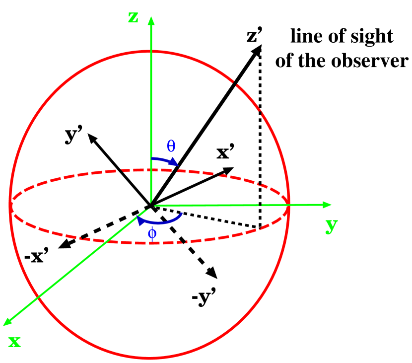
We introduce two Cartesian coordinate systems, $\vec{x}=(x,y,z)$ and $\vec{x^{\prime}}=(x^{\prime},y^{\prime},z^{\prime})$, which represent respectively the principal coordinate system of the triaxial dark halo and the observer’s coordinate system. The origins of both coordinate systems are set at the center of the halo. It is assumed that the $z^{\prime}$-axis runs along the line-of-sight direction of the observer, and that the $z$-axis lies along the major principal axis. In general, the relative orientation between the two coordinate systems can be specified by the three Euler angles. However, in our case, it is only the line-of-sight direction that is fixed while the rotation angle of the $x^{\prime}$-$y^{\prime}$ plane relative to $x$-$y$ plane is arbitrary, and thus we may need only two angles to specify the relative orientation of the two coordinate systems. Here we make a choice of $x^{\prime}$-axis lying in the $x$-$y$ plane. Then the relative orientation of the two coordinate systems can be expressed in terms of the line-of-sight direction in the halo principal coordinate system.

Let $(\theta,\phi)$ be the polar coordinates of the line-of-sight direction in the $\vec{x}$-coordinate system. Then the relation between the two coordinate systems can be expressed in terms of the rotation matrix $A$ (Binney, 1985) as

$$\vec{x}=A\vec{x^{\prime}},$$ (1)

where

$$A\equiv\left(\begin{array}[]{ccc}-\sin\phi&-\cos\phi\cos\theta&\cos\phi\sin\theta\\ \cos\phi&-\sin\phi\cos\theta&\sin\phi\sin\theta\\ 0&\sin\theta&\cos\theta\\ \end{array}\right).$$ (2)

Figure 1 represents the relative orientation between the observer’s coordinate system and the halo principal coordinate system.

Figure 1: The orientations of the coordinate systems. The Cartesian axes ($x,y,z$) represent the halo principal coordinate system while the axes ($x^{\prime},y^{\prime},z^{\prime}$) stand for the observers coordinate system with $z^{\prime}$-axis aligned with the line-of-sight direction. The $x^{\prime}$-axis lies in the $x$-$y$ plane. The angle $(\theta,\phi)$ represent the polar angle of the line-of-sight direction in the $(x,y,z)$-coordinate system.

2.2 Density Profile of Triaxial Dark Matter Halos

We adopt the following density profiles of triaxial dark matter halos proposed by JS02:

$$\rho(R)=\frac{\delta_{\rm ce}\rho_{\rm crit}(z)}{(R/R_{0})^{\alpha}(1+R/R_{0})^{3-\alpha}},$$ (3)

where

$$R^{2}\equiv c^{2}\left(\frac{x^{2}}{a^{2}}+\frac{y^{2}}{b^{2}}+\frac{z^{2}}{c^{2}}\right)\;\;\;(a\leq b\leq c).$$ (4)

The precise value of the inner slope, $\alpha$, is still controversial, but almost all the N-body simulations based on the collisionless CDM scenario indicate values between $1$ and $1.5$ (Navarro et al., 1996, 1997; Moore et al., 1999; Jing & Suto, 2000; Fukushige & Makino, 2001, 2003; Power et al., 2003). Thus we consider both $\alpha=1$ and $\alpha=1.5$ below so as to cover a possible range of the CDM predictions proposed so far.

JS02 defined the concentration parameter in the triaxial model as

$$c_{e}\equiv\frac{R_{e}}{R_{0}},$$ (5)

where $R_{e}$ is chosen so that the mean density within the ellipsoid of the major axis radius $R_{e}$ is $\Delta_{e}\Omega(z)\rho_{\rm crit}(z)$ with

$$\Delta_{e}=5\Delta_{\rm vir}\left(\frac{c^{2}}{ab}\right)^{0.75}.$$ (6)

Here $\Omega(z)$ and $\rho_{\rm crit}(z)$ denote the matter density parameter and the critical density of universe at redshift $z$, respectively, and $\Delta_{\rm vir}(z)$ denotes the overdensity of objects virialized at $z$ whose approximate expression is found, e.g., in Oguri et al. (2001).

Then the characteristic density $\delta_{\rm ce}$ in equation (3) is written in terms of the concentration parameter $c_{e}$ as

$$\delta_{\rm ce}=\frac{\Delta_{e}\Omega(z)}{3}\frac{c_{e}^{3}}{m(c_{e})},$$ (7)

where $m(c_{e})$ is

$$m(c_{e})\equiv\frac{c_{e}^{3-\alpha}}{3-\alpha}\,{}_{2}F_{1}\left(3-\alpha,3-\alpha;4-\alpha;-c_{e}\right),$$ (8)

with ${}_{2}F_{1}\left(a,b;c;x\right)$ being the hypergeometric function. For $\alpha=1$ and $1.5$, equation (8) simply reduces to

$$m(c_{e})=\left\{\begin{array}[]{ll}\displaystyle{\ln(1+c_{e})-\frac{c_{e}}{1+c_{e}}}&\mbox{($\alpha=1$)},\\ \displaystyle{2\ln(\sqrt{c_{e}}+\sqrt{1+c_{e}})-2\sqrt{\frac{c_{e}}{1+c_{e}}}}&\mbox{($\alpha=1.5$)}.\end{array}\right.$$ (11)

Since $R_{e}$ is empirically related to the (spherical) virial radius $r_{\rm vir}$ as $R_{e}/r_{\rm vir}\simeq 0.45$ (JS02), the scaling radius in the triaxial model, $R_{0}$, for a halo of a mass $M_{\rm vir}$ is given as

$$R_{0}=0.45\frac{r_{\rm vir}}{c_{e}}=\frac{0.45}{c_{e}}\left(\frac{3M_{\rm vir}}{4\pi\Delta_{\rm vir}\Omega(z)\rho_{\rm crit}(z)}\right)^{1/3}.$$ (12)

Since we do not know the properties of the density profile of an individual lensing halo, our prediction for the number of arcs is necessarily statistical in a sense that it should be made after averaging over appropriate PDFs of the properties of halos. For this purpose, we adopt the PDFs that JS02 empirically derived from their simulations. For the axis ratios, they are given as

$$p(a/c)=\frac{1}{\sqrt{2\pi}\times 0.113}\exp\left[-\frac{\left\{(a/c)(M_{\rm vir}/M_{*})^{0.07[\Omega(z)]^{0.7}}-0.54\right\}^{2}}{2(0.113)^{2}}\right]\left(\frac{M_{\rm vir}}{M_{*}}\right)^{0.07[\Omega(z)]^{0.7}},$$ (13)

and

$$p(a/b|a/c)=\frac{3}{2(1-\max(a/c,0.5))}\left[1-\left(\frac{2a/b-1-\max(a/c,0.5)}{1-\max(a/c,0.5)}\right)^{2}\right],$$ (14)

for $a/b\geq\max(a/c,0.5)$, and $p(a/b|a/c)=0$ otherwise (JS02). Here $M_{*}$ is the characteristic nonlinear mass so that the rms top-hat smoothed overdensity at that mass scale is $1.68$. For the concentration parameter, we adopt

$$p(c_{e})=\frac{1}{\sqrt{2\pi}\times 0.3}\exp\left[-\frac{(\ln c_{e}-\ln\bar{c}_{e})^{2}}{2(0.3)^{2}}\right]\frac{1}{c_{e}},$$ (15)

where the fit to the median concentration parameter $\bar{c}_{e}$ for $\alpha=1$ is given as :

$$\bar{c}_{e}=1.35\exp\left[-\left\{\frac{0.3}{(a/c)(M_{\rm vir}/M_{*})^{0.07[\Omega(z)]^{0.7}}}\right\}^{2}\right]A_{e}\sqrt{\frac{\Delta_{\rm vir}(z_{c})}{\Delta_{\rm vir}(z)}}\left(\frac{1+z_{c}}{1+z}\right)^{3/2},$$ (16)

with $z_{c}$ being the collapse redshift of the halo of mass $M_{\rm vir}$ (JS02). In the case of $\alpha=1$, we simply use the above expression, and for $\alpha=1.5$, we use the relation $\bar{c}_{e}(\alpha=1.5)=0.5\bar{c}_{e}(\alpha=1)$ (Keeton & Madau 2001; JS02). JS02 estimated $A_{e}=1.1$ in the Lambda-dominated CDM model, but this value is likely to be dependent on the underlying cosmology to some extent. As we stressed in Introduction, however, we do not intend to survey the cosmological parameters but rather focus on the effects of the properties of the lensing halos. Therefore while we mostly fix the value $A_{e}=1.1$, we also vary the value between 0.8 and 1.6 to see its systematic effect in §6. Incidentally this is useful in understanding the difference of the predicted number of arcs between open and Lambda-dominated CDM models found by Bartelmann et al. (1998).

3 Gravitational Lensing by Triaxial Dark Matter Halos

In this section, we present several expressions for triaxial dark matter halos which are useful in calculating gravitational lensing properties. Under the thin lens approximation, gravitational lensing properties are fully characterized by the matter density projected along the line-of-sight (e.g., Schneider, Ehlers, & Falco, 1992). We have to calculate the mass density profile projected along the arbitrary line-of-sight directions, because the line-of-sight, in general, does not coincide with the principal axis of a triaxial dark matter halo.

For simplicity, in this section we redefine $\vec{x}/R_{0}$ and $\vec{x^{\prime}}/R_{0}$ as $\vec{x}$ and $\vec{x^{\prime}}$, respectively. In this case,

$$\rho(R)=\frac{\delta_{\rm ce}\rho_{\rm crit}(z)}{R^{\alpha}(1+R)^{3-\alpha}},$$ (17)

with $R$ being defined by equation (4). In terms of the observer’s coordinates $(x^{\prime},y^{\prime},z^{\prime})$, $R$ is written as

$$R=\sqrt{fz^{\prime 2}+gz^{\prime}+h},$$ (18)

where

$$f = \sin^{2}\theta\left(\frac{c^{2}}{a^{2}}\cos^{2}\phi+\frac{c^{2}}{b^{2}}\sin^{2}\phi\right)+\cos^{2}\theta,$$ (19)

$$g = \sin\theta\sin 2\phi\left(\frac{c^{2}}{b^{2}}-\frac{c^{2}}{a^{2}}\right)x^{\prime}+\sin 2\theta\left(1-\frac{c^{2}}{a^{2}}\cos^{2}\phi-\frac{c^{2}}{b^{2}}\sin^{2}\phi\right)y^{\prime},$$ (20)

$$h = \left(\frac{c^{2}}{a^{2}}\sin^{2}\phi+\frac{c^{2}}{b^{2}}\cos^{2}\phi\right)x^{\prime 2}+\sin 2\phi\cos\theta\left(\frac{c^{2}}{a^{2}}-\frac{c^{2}}{b^{2}}\right)x^{\prime}y^{\prime}+\left[\cos^{2}\theta\left(\frac{c^{2}}{a^{2}}\cos^{2}\phi+\frac{c^{2}}{b^{2}}\sin^{2}\phi\right)+\sin^{2}\theta\right]y^{\prime 2}.$$ (21)

Defining two new variables $z^{\prime}_{*}{}^{2}$ and $\zeta$

$$z^{\prime}_{*}{} \equiv \sqrt{f}\left(z^{\prime}+\frac{g}{2f}\right),$$ (22)

$$\zeta \equiv h-\frac{g^{2}}{4f},$$ (23)

we rewrite equation (18) as

$$R=\sqrt{z^{\prime}_{*}{}^{2}+\zeta^{2}}.$$ (24)

Then the convergence $\kappa$ can be expressed as a function of $\zeta$:

$$\kappa=\frac{R_{0}}{\Sigma_{\rm crit}}\int_{-\infty}^{\infty}\rho(R)dz^{\prime}=\frac{R_{0}}{\Sigma_{\rm crit}}\int_{-\infty}^{\infty}\frac{1}{\sqrt{f}}\rho\left(\sqrt{z^{\prime}_{*}{}^{2}+\zeta^{2}}\right)dz^{\prime}_{*}\equiv\frac{b_{\rm TNFW}}{2}f_{\rm GNFW}(\zeta),$$ (25)

where

$$b_{\rm TNFW}\equiv\frac{1}{\sqrt{f}}\frac{4\delta_{\rm ce}\rho_{\rm crit}(z)R_{0}}{\Sigma_{\rm crit}},$$ (26)

and

$$f_{\rm GNFW}(r)\equiv\int_{0}^{\infty}\frac{1}{\left(\sqrt{r^{2}+z^{2}}\right)^{\alpha}\left(1+\sqrt{r^{2}+z^{2}}\right)^{3-\alpha}}dz.$$ (27)

The critical surface mass density $\Sigma_{\rm crit}$ is defined by

$$\Sigma_{\rm crit}\equiv\frac{c^{2}D_{\rm OS}}{4\pi GD_{\rm OL}D_{\rm LS}},$$ (28)

where $D_{\rm OL}$, $D_{\rm OS}$, and $D_{\rm LS}$ denote the angular diameter distances from the observer to the lens plane, from the observer to the source plane, and from the lens plane to the source plane, respectively.

The meaning of the variable $\zeta$ can be easily understood by substituting equations (19)-(21) into equation (23):

$$\zeta^{2}=\frac{1}{f}\left(Ax^{\prime 2}+Bx^{\prime}y^{\prime}+Cy^{\prime 2}\right),$$ (29)

where

$$A \equiv \cos^{2}\theta\left(\frac{c^{2}}{a^{2}}\sin^{2}\phi+\frac{c^{2}}{b^{2}}\cos^{2}\phi\right)+\frac{c^{2}}{a^{2}}\frac{c^{2}}{b^{2}}\sin^{2}\theta,$$ (30)

$$B \equiv \cos\theta\sin 2\phi\left(\frac{c^{2}}{a^{2}}-\frac{c^{2}}{b^{2}}\right),$$ (31)

$$C \equiv \frac{c^{2}}{b^{2}}\sin^{2}\phi+\frac{c^{2}}{a^{2}}\cos^{2}\phi.$$ (32)

The quadratic form of equation (29) implies that the iso-$\zeta$ curves are ellipses, and that the position angle of ellipses $\psi$ is

$$\psi=\frac{1}{2}\arctan\frac{B}{A-C}.$$ (33)

By rotating the $x^{\prime}y^{\prime}$-plane by the angle $\psi$, we diagonalize equation (29) such that

$$\zeta^{2}=\frac{x^{\prime 2}}{q_{x}^{2}}+\frac{y^{\prime 2}}{q_{y}^{2}},$$ (34)

where

$$q_{x}^{2} \equiv \frac{2f}{A+C-\sqrt{(A-C)^{2}+B^{2}}},$$ (35)

$$q_{y}^{2} \equiv \frac{2f}{A+C+\sqrt{(A-C)^{2}+B^{2}}}.$$ (36)

Note that $q_{x}\geq q_{y}$ for the given $\psi$. We further define the axis ratio $q$ as

$$q\equiv\frac{q_{y}}{q_{x}}=\left(\frac{A+C-\sqrt{(A-C)^{2}+B^{2}}}{A+C+\sqrt{(A-C)^{2}+B^{2}}}\right)^{1/2},$$ (37)

which represents the ellipticities of the projected isodensity curves of the triaxial dark halos. In this case, the convergence $\kappa$ is expressed as $\kappa=\kappa(\xi)$, where $\xi^{2}=x^{\prime}{}^{2}+y^{\prime}{}^{2}/q^{2}$. The advantage of this diagonalization is that we can apply the previous method to calculate lensing properties (Schramm, 1990; Keeton, 2001a) where the deflection angle $\vec{\beta}=(\beta_{x^{\prime}},\beta_{y^{\prime}})$ is expressed as a one-dimensional integral of the convergence $\kappa(\xi)$:

$$\beta_{x^{\prime}}(x^{\prime},y^{\prime}) = qx^{\prime}J_{0}(x^{\prime},y^{\prime}),$$ (38)

$$\beta_{y^{\prime}}(x^{\prime},y^{\prime}) = qy^{\prime}J_{1}(x^{\prime},y^{\prime}),$$ (39)

where the integral $J_{n}(x,y)$ is

$$J_{n}(x,y)=\int_{0}^{1}\frac{\kappa\left(\xi(v)\right)}{\left[1-(1-q^{2})v\right]^{n+1/2}}dv,$$ (40)

and $\xi(v)$ is

$$\xi^{2}(v)=v\left(x^{2}+\frac{y^{2}}{1-(1-q^{2})v}\right).$$ (41)

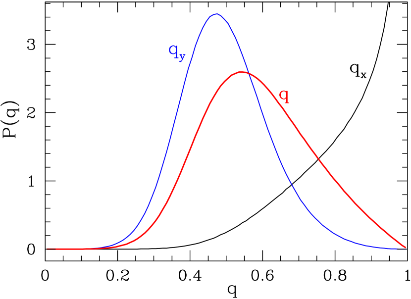
Figure 2 plots PDFs of $q$, $q_{x}$, and $q_{y}$. They were computed numerically using equations (13)-(14) and (35)-(37) under the assumption that the triaxial halo orientations (i.e., the angles $\theta$ and $\phi$) are randomly distributed. In this plot we set $M_{\rm vir}=10^{15}h^{-1}M_{\odot}$ and $z=0.3$, which are s typical mass scale and a redshift of lensing clusters. It is clear from Figure 2 that the axis ratio of projected isodensity contours strongly deviates from unity, having maximum around $q\sim 0.6$. This large degree of ellipticity suggests that the triaxial dark halos in realistic cosmological models significantly enhances the number of arcs compared with the conventional spherical model predictions.

Figure 2: PDFs of $q$ (eq. [37]) , $q_{x}$ (eq. [35]), and $q_{y}$ (eq. [36]). Here we consider a halo with mass $M_{\rm vir}=10^{15}h^{-1}M_{\odot}$ and redshift $z=0.3$, but the result only weakly depends on the halo mass and redshift. These PDFs are calculated from PDFs of axis ratios $p(a/c)$ and $p(a/b)$ for which we use equations (13) and (14). We assume that the orientations of dark halos are random.

For $\alpha=1$, $f_{\rm GNFW}(r)$ defined in equation (27) is analytically expressed as (Bartelmann, 1996):

$$f_{\rm GNFW}(r)=\left\{\begin{array}[]{ll}{\displaystyle\frac{1}{1-r^{2}}\left[-1+\frac{2}{\sqrt{1-r^{2}}}{\rm arctanh}\sqrt{\frac{1-r}{1+r}}\right]}&\mbox{($r<1$),}\\ {\displaystyle\frac{1}{r^{2}-1}\left[1-\frac{2}{\sqrt{r^{2}-1}}\arctan\sqrt{\frac{r-1}{r+1}}\right]}&\mbox{($r>1$),}\end{array}\right.$$ (44)

but it does not has a simple analytical expression for $\alpha=1.5$. Thus we use the following fitting formula in this case:

$$f_{\rm GNFW}(r)=\frac{2.614}{r^{0.5}\left(1+2.378r^{0.5833}+2.617r^{1.5}\right)}.$$ (45)

The error of the above fit is $\lesssim 0.6$%.

4 Arc Statistics in the Triaxial Dark Matter Halo

4.1 Cross Sections for Arcs from the Monte Carlo Simulation

First we compute the cross section for arcs without distinguishing tangential and radial arcs mainly because of the computational cost. In fact, the previous analyses indicate that while the number ratio of radial to tangential arcs offers another information on the density profile, the ratio is rather insensitive to the non-sphericity (Molikawa & Hattori, 2001; Oguri et al., 2001; Oguri, 2002a).

Since the analytical computation of the cross sections is not practically feasible except for spherical models, we resort to the direct Monte Carlo method (Bartelmann & Weiss, 1994; Miralda-Escudé, 1993b; Molikawa & Hattori, 2001; Oguri, 2002a). We showed that the convergence of triaxial dark matter halos is expressed by equation (25). Thus the corresponding lensing deflection angle $\vec{\alpha}$, and therefore the cross section $\tilde{\sigma}$, are fully characterized by the two parameters, $b_{\rm TNFW}$ and $q$, as long as the finite size of source galaxies is safely neglected. Thus we perform the Monte Carlo simulations on the dimensionless $X$-$Y$ plane, where $X$ and $Y$ are $X\equiv x^{\prime}/(R_{0}q_{x})$ and $Y\equiv y^{\prime}/(R_{0}q_{x})$, and tabulate the deflection angle and the dimensionless cross section

$$\vec{\alpha} = \vec{\alpha}(b_{\rm TNFW},q),$$ (46)

$$\tilde{\sigma} = \tilde{\sigma}(b_{\rm TNFW},q),$$ (47)

in $50\times 19$ bins ($\alpha=1$) or $70\times 19$ bins ($\alpha=1.5$) for $b_{\rm TNFW}$ and $q$, respectively. The dimensionless cross section is translated to the dimensional one in the source plane as

$$\sigma=\tilde{\sigma}(b_{\rm TNFW},q)\times\left(R_{0}q_{x}\frac{D_{\rm OS}}{D_{\rm OL}}\right)^{2}.$$ (48)

Figure 3: Contours of dimensionless cross sections $\tilde{\sigma}$ and average magnification factors $\langle\mu\rangle$ in the $q$-$b_{\rm TNFW}$ plane for $\alpha=1$. The threshold axis ratios for arcs are set to $\epsilon_{\rm th}=10$ (upper) and $7$ (lower), respectively. Contours are drawn at $10^{0.5n}$ for $\tilde{\sigma}$ and at $10^{0.125n}$ for $\langle\mu\rangle$, where $n$ is integer. When $n$ is in multiples of $4$, contours are drawn by thick lines. These cross sections and magnification factors are derived from Monte Carlo simulations described in §4.1.

Figure 4: Same as Figure 3, except for $\alpha=1.5$.

We follow the simulation method by Oguri (2002a) which is briefly summarized below. We use a $2048\times 2048$ regular grid on the $X$-$Y$ plane and calculate the deflection angle at each grid point. The box size is adjusted so as to include all arcs in the box for each $(b_{\rm TNFW},q)$. Therefore, the box size almost scales as the tangential critical line for each $(b_{\rm TNFW},q)$. After those deflection angles are obtained at each grid point, we trace back the corresponding position in the source plane, and see whether or not it constitutes a part of lensed images. In order to take account of the source ellipticity which is also important in arc statistics (Keeton, 2001b), we assume that it distributes randomly in the range of [0,0.5], where source ellipticity is defined by $1-b_{\rm s}/a_{\rm s}$ with $a_{\rm s}$ and $b_{\rm s}$ being semi-major and semi-minor axes, respectively. We adopt this distribution of intrinsic ellipticities in order to compare our results with the previous works (e.g., Bartelmann et al., 1998) in which the same distribution was assumed. Moreover, the distribution is roughly consistent with the observed distribution (e.g., Lambas, Maddox, & Loveday, 1992). Once we identify a lensed image, we compute its length $l$ and width $w$ as described in Oguri (2002a). Finally we define a lensed arc if the ratio of $l$ and $w$ exceeds the threshold value $\epsilon_{\rm th}$ that we set:

$$\frac{l}{w}\geq\epsilon_{\rm th}.$$ (49)

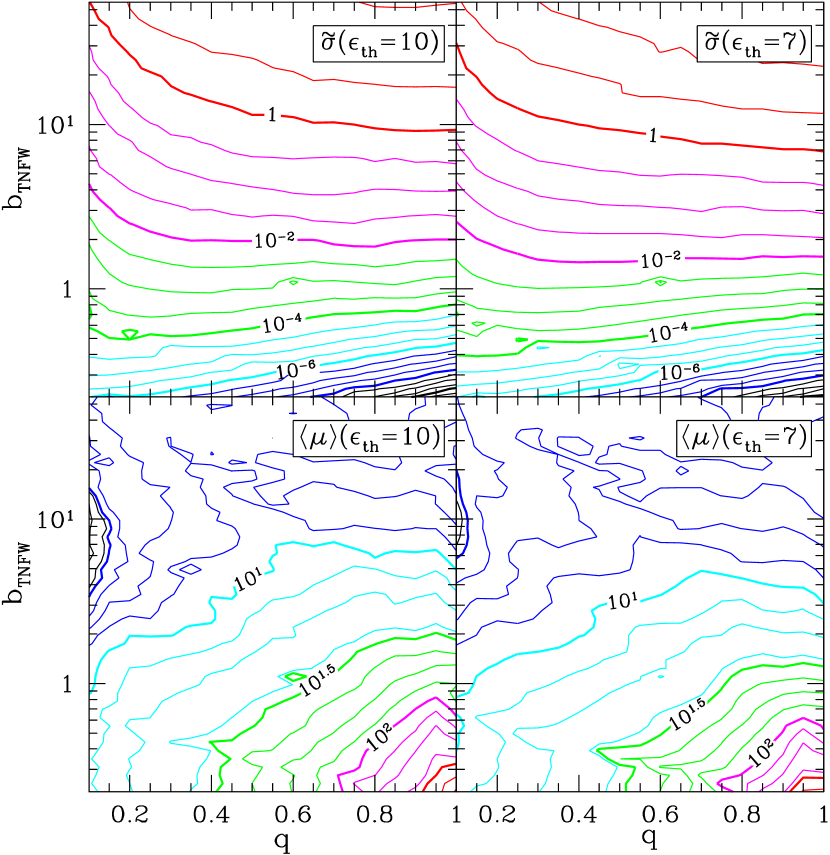
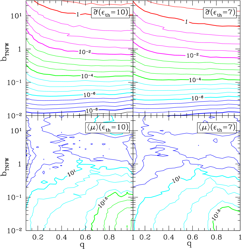
In practice, we consider $\epsilon_{\rm th}=7$ and $10$ to check the robustness of the conclusion. We also compute the average magnification of the arcs $\langle\mu\rangle$ for each set of $(b_{\rm TNFW},q)$ which is required in estimating the magnification bias (Turner, 1980; Turner, Ostriker, & Gott, 1984). The contours of the lensing cross sections and the average magnification are plotted in Figures 3 and 4 for $\alpha=1$ and $\alpha=1.5$, respectively. We confirmed that the cross sections for $q=1$ cases reproduce the analytic result of spherical lens models for point source.

We should note that our current method does not take account of the finite size effect of source galaxies, and thus our results are, strictly speaking, applicable only to a sufficiently small source. Since the number of tangential arcs, which dominates the total number of arcs, is known to be insensitive to the source size (Hattori et al., 1997b; Bartelmann et al., 1998; Molikawa & Hattori, 2001; Oguri et al., 2001; Oguri, 2002a), this should not change our conclusion.

4.2 Predicting Numbers of Arcs

The next step is to average the cross section for arcs corresponding to a halo of $M_{\rm vir}$ at $z_{\rm L}$ and a galaxy at $z_{\rm S}$ over the halo properties (its orientations and axis ratios):

$$\overline{\sigma}(M_{\rm vir},z_{\rm L},z_{\rm S})=\int d(a/c)\int dc_{e}\int d(a/b)\int d\theta\int d\phi~{}p(a/c)p(c_{e})p(a/b|a/c)p(\theta)p(\phi)\sigma.$$ (50)

In what follows, we assume the orientations of triaxial dark matter halos are completely random:

$$p(\theta) = \frac{\sin\theta}{2},$$ (51)

$$p(\phi) = \frac{1}{2\pi}.$$ (52)

The realistic prediction for the number of arcs also requires to properly take account of the magnification bias. Thus we use the average of the cross section times number density of galaxies above the magnitude limit:

$$\overline{\sigma n_{\rm g}}(M_{\rm vir},z_{\rm L},z_{\rm S})=\int d(a/c)\int dc_{e}\int d(a/b)\int d\theta\int d\phi p(a/c)\,p(c_{e})\,p(a/b|a/c)\,p(\theta)\,p(\phi)\,\sigma\int_{L_{\rm min}}^{\infty}dLn_{g}(L,z_{\rm S}),$$ (53)

where $n_{g}(L,z)$ is the luminosity function of source galaxies for which we adopt the Schechter form:

$$n_{g}(L,z)dL=\phi^{*}\left(\frac{L}{L^{*}}\right)^{\alpha_{\rm s}}\exp\left(-\frac{L}{L^{*}}\right)\frac{dL}{L^{*}}.$$ (54)

Its integral over $L$ simply reduces to

$$\int_{L_{\rm min}}^{\infty}dL\,n_{g}(L,z_{\rm S})=\phi^{*}\Gamma(\alpha_{\rm s}+1,L_{\rm min}/L^{*}),$$ (55)

with $\Gamma(a,x)$ being the incomplete gamma function of the second kind. The lower limit of the integral, $L_{\rm lim}$, may be computed from limiting magnitude of observation, $m^{*}$, and the lensing magnification factor $\langle\mu\rangle$ (see Figs. 3 and 4):

$$\frac{L_{\rm min}}{L^{*}} = \frac{10^{-0.4(m_{\rm lim}-m^{*})}}{\langle\mu\rangle},$$ (56)

$$m^{*} = M^{*}+5\log\left[\frac{D_{\rm OS}(1+z_{\rm S})^{2}}{10{\rm pc}}\right]+K(z_{\rm S}).$$ (57)

We adopt the K-correction in B-band for spiral galaxies (King & Ellis, 1985):

$$K(z)=-0.05+2.35z+2.55z^{2}-4.89z^{3}+1.85z^{4}.$$ (58)

Finally the number distribution of lensed arcs for a halo of mass $M_{\rm vir}$ at $z_{\rm L}$ is given by

$$\frac{dN_{\rm arc}}{dz_{\rm S}}(z_{\rm S};M_{\rm vir},z_{\rm L})=\overline{\sigma n_{\rm g}}(M_{\rm vir},z_{\rm L},z_{\rm S})\frac{cdt}{dz_{\rm S}}(1+z_{\rm S})^{3},$$ (59)

and the total number of lensed arcs for the halo is

$$N_{\rm arc}(M_{\rm vir},z_{\rm L})=\int_{z_{\rm L}}^{z_{\rm S,max}}dz_{\rm S}\,\frac{dN_{\rm arc}}{dz_{\rm S}}(z_{\rm S};M_{\rm vir},z_{\rm L}).$$ (60)

While the upper limit of redshifts of source galaxies, $z_{\rm S,max}$, is in principle arbitrary, it is practically limited by the validity of the input luminosity function of source galaxies and the applied K-correction at high redshifts. In the present analysis, we conservatively set $z_{\rm S,max}=1.25$ because of the K-correction (eq. [58]) and the luminosity function (§4.3). Nevertheless we stress here that our methodology can be applied to at higher redshifts if they are replaced by any reliable models valid there.

4.3 Luminosity Function of Source Galaxies

While the predicted number of arcs sensitively depends on the luminosity function of source galaxies (e.g., Hamana & Futamase, 1997), $n_{\rm g}(L.z)$ is still fairly uncertain especially at high $z$. Thus we consider the following four luminosity functions measured up to $z=1.25$: HDF1 from the Hubble Deep Field and the New Technology Telescope Deep Field (Poli et al., 2001), HDF2 from the Hubble Deep Field (Sawicki, Lin, & Yee, 1997), SDF from the Subaru Deep Field (Kashikawa et al., 2003), and CFRS from the Canada-France Redshift Survey (Lilly et al., 1995). They are summarized in Table Arc Statistics in Triaxial Dark Matter Halos: Testing the Collisionless Cold Dark Matter Paradigm. Although the Schechter fits to those luminosity functions are valid only at $z>(0.2\sim 0.6)$, we simply extrapolate the values even down to $z=0$ if necessary. This does not affect our result in §5 at all since galaxies at $z\sim 1$ are the main sources of lensed arcs for our sample of clusters at $z>0.2$ (§5.1).

Except for HDF1, the Schechter parameters were derived assuming the Einstein-de Sitter (EdS) model ($\Omega_{0}=1$, $\lambda_{0}=0$) in the original references. We convert them into the counterparts in the Lambda-dominated universe ($\Omega_{0}=0.3$, $\lambda_{0}=0.7$) as follows.

Since the number of galaxies in the redshift interval $[z_{\rm S},z_{\rm S}+dz_{\rm S}]$,

$$dN_{\rm g}(z_{\rm S})\propto D^{2}_{\rm OS}\frac{c\,dt}{dz_{\rm S}}dz_{\rm S}n_{\rm g}(L,z_{\rm S})dL,$$ (61)

is observable, it should be invariant. Thus the luminosity function in the Lambda-dominated universe is related to that in the EdS as:

$$\left[n_{\rm g}(L^{\prime},z_{\rm S})dL^{\prime}\right]_{\rm Lambda}=\frac{\left[D^{2}_{\rm OS}(c\,dt/dz_{\rm S})\right]_{\rm EdS}}{\left[D^{2}_{\rm OS}(c\,dt/dz_{\rm S})\right]_{\rm Lambda}}\left[n_{\rm g}(L,z_{\rm S})dL\right]_{\rm EdS},$$ (62)

where

$$L^{\prime}\equiv\frac{\left[D^{2}_{\rm OS}\right]_{\rm Lambda}}{\left[D^{2}_{\rm OS}\right]_{\rm EdS}}L.$$ (63)

Figure 5: Luminosity functions of source galaxies (eq. [64]) for $z=0.3$, $0.6$, $0.9$, and $1.2$. Parameters of these luminosity functions are summarized in Table Arc Statistics in Triaxial Dark Matter Halos: Testing the Collisionless Cold Dark Matter Paradigm.

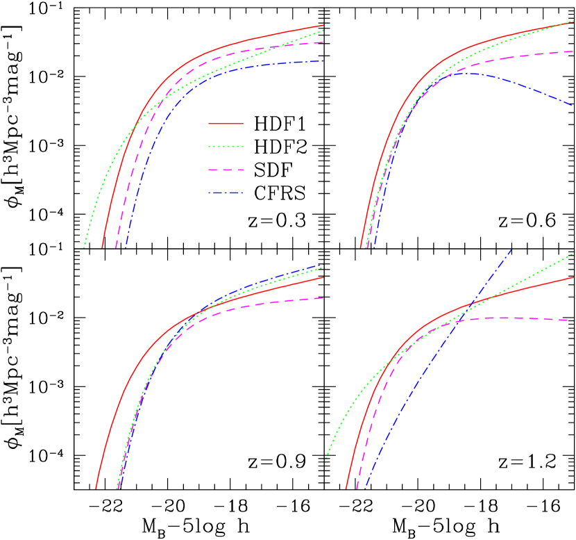
The resulting luminosity functions in terms of the absolute magnitude $M$:

$$\phi_{M}(M,z)dM=0.921\phi^{*}10^{-0.4(\alpha_{\rm s}+1)(M-M^{*})}\exp\left(-10^{-0.4(M-M^{*})}\right)dM,$$ (64)

at $z=0.3$, $0.6$, $0.9$, and $1.2$ are plotted in Figure 5. Clearly the uncertainty increases at fainter luminosities at $z>1$, which may significantly change the predicted number of arcs. Therefore, while we adopt HDF1 as our fiducial model, we also attempt to evaluate the uncertainty due to the different choice of luminosity functions using the other three.

4.4 Predicted Cross Sections and Numbers of Arcs

Figure 6: Average cross sections (eq. [50]) for triaxial and spherical dark matter halo models as a function of source redshift $z_{\rm S}$ for both $\alpha=1$ (left) and $1.5$ (right), where $\alpha$ is the inner slope of dark matter halo density profile. The lens cluster has a mass $M_{\rm vir}=10^{15}h^{-1}M_{\odot}$ and is placed at $z_{\rm L}=0.3$. For the threshold axis ratio of arcs, we adopt both $\epsilon_{\rm th}=10$ (solid) and $7$ (dashed).

Figure 7: Number distributions of arcs (eq. [59]) for triaxial and spherical dark matter halo models. The B-band magnitude limit for arcs is set to $m_{\rm lim}=24$. The distributions are discontinuous at $z_{\rm S}=0.75$ because we adopt binned luminosity function (see Table Arc Statistics in Triaxial Dark Matter Halos: Testing the Collisionless Cold Dark Matter Paradigm).

Figure 8: Predicted numbers of arcs (eq. [60]) as a function of halo mass $M_{\rm vir}$. The redshift of the dark halo is still fixed to $z_{\rm L}=0.3$. The B-band magnitude limit for arcs is set to $m_{\rm lim}=24$.

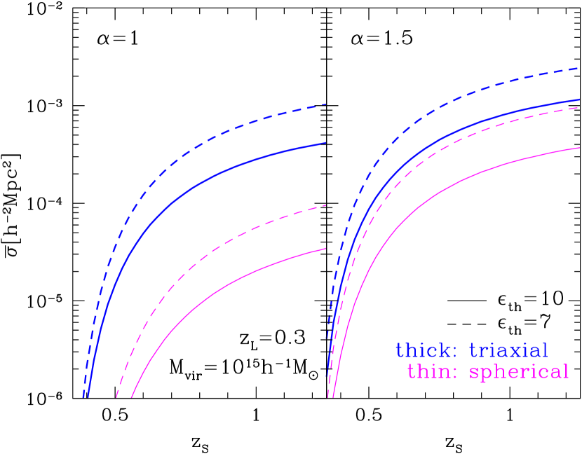
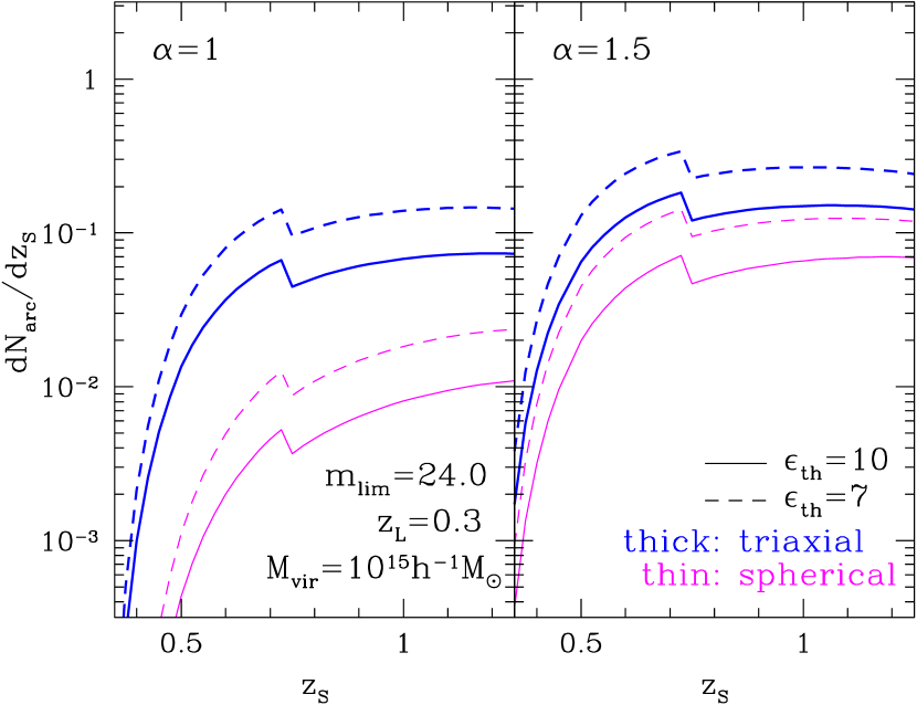
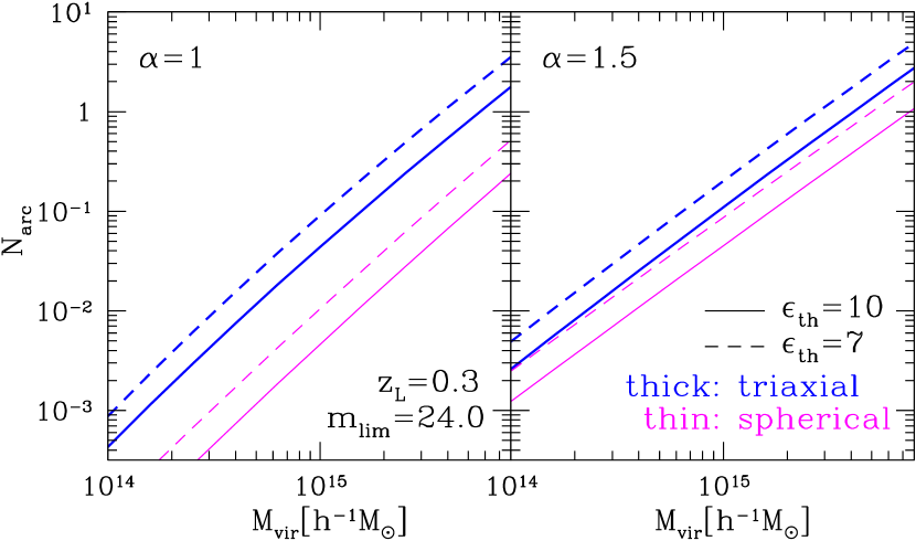
Figure 6 shows the average cross sections (eq. [50]) of a dark matter halo of $M_{\rm vir}=10^{15}h^{-1}M_{\odot}$ at $z_{\rm L}=0.3$. The cross section for the triaxial model is larger by a factor of 10 ($\alpha=1$) and of 4 ($\alpha=1.5$) than that for the spherical counterpart. Since the magnification factor is always larger for smaller cross sections (see Figures 3 and 4), the magnification bias further reduces the difference between $\alpha=1$ and 1.5 for the triaxial model. This explains the behavior of Figure 7 where the source redshift distribution of arcs (eq. [59]) is plotted. Actually the figure indicates that the non-spherical effect even exceeds that of the difference due to the inner slope.

Figure 9: Predicted numbers of arcs as a function of B-band magnitude limit $m_{\rm lim}$. The mass of lens cluster is $M_{\rm vir}=10^{15}h^{-1}M_{\odot}$.

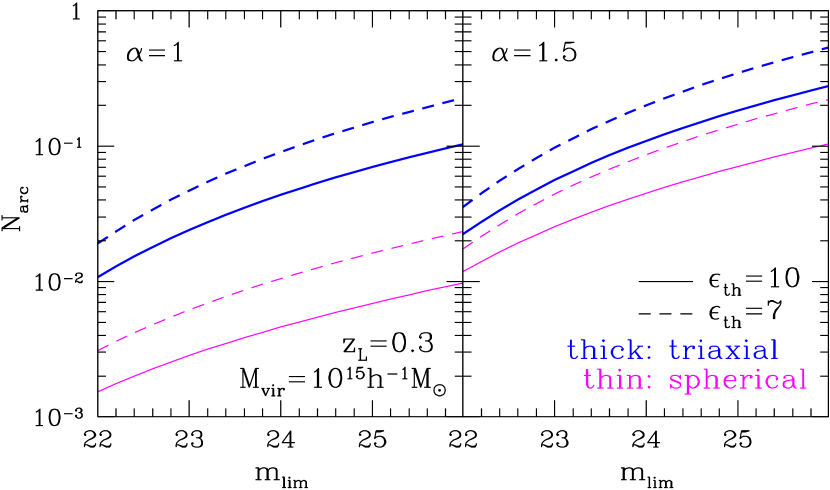
Figures 8, 9 and 10 show how the predicted number of arcs depends on the mass of a lensing halo, the limiting magnitude of the survey, and the adopted luminosity function of source galaxies. Figure 8 shows that the number of arcs is sensitive to the mass of halo, implying the estimate of the mass of the target cluster is essential in interpreting the data. In addition, the difference between $\alpha=1$ and 1.5 becomes smaller for the triaxial model of $M_{\rm vir}>10^{15}M_{\odot}$. Thus in order to distinguish the inner slope clearly as well, one needs a sample of less massive clusters that have lensed arcs.

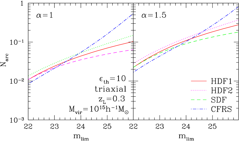
Figure 9 indicates that the number of arcs is also sensitive to the magnitude limit, suggesting that the well-controlled selection function for the arc survey is quite important. On the other hand, the uncertainty of the luminosity function of source galaxies seems to be less critical, at least for arcs of galaxies at $z_{\rm s}<1.25$ that we consider in this paper (Fig. 10). The difference among the four luminosity functions (see Table Arc Statistics in Triaxial Dark Matter Halos: Testing the Collisionless Cold Dark Matter Paradigm) is merely up to 50 % for $m_{\rm lim}<24$, and is within a factor of 2 even at $m_{\rm lim}<26$ except CFRS. The predictions based on HDF1 approximately correspond to the median among the four and this is why we choose this as our fiducial model in what follows.

Figure 10: Predicted numbers of arcs for different luminosity functions of source galaxies as a function of B-band magnitude limit $m_{\rm lim}$. Parameters of luminosity functions are given in Table Arc Statistics in Triaxial Dark Matter Halos: Testing the Collisionless Cold Dark Matter Paradigm. Only triaxial dark matter halo model and threshold axis ratio $\epsilon_{\rm th}=10$ are considered.

5 Comparison with the Observed Number of Arcs

5.1 Cluster Data

We use a sample of $38$ X-ray selected clusters compiled by Luppino et al. (1999). The clusters are selected from the Einstein Observatory Extended Medium Sensitivity Survey (EMSS). For all the clusters, deep imaging observations with B-band limiting magnitude $m_{\rm lim}\sim 26.0$ were carried out to search for arcs.

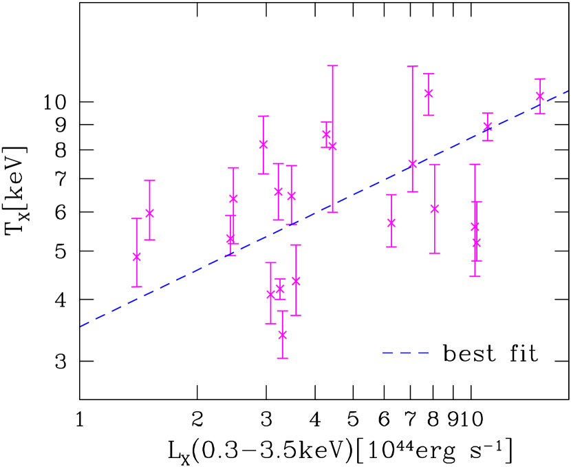
As we remarked in the previous section, the mass estimate of those clusters is important in understanding the implications from the observed arcs statistics. For this purpose, we first construct a gas temperature – X-ray luminosity (in the Einstein band) relation from a subset of the above clusters whose temperature is determined. Then we estimate the temperature of the remaining clusters using the temperature – luminosity relation. Finally we estimate the mass of each cluster employing the virial mass – gas temperature relation of Finoguenov, Reiprich, & Böhringer (2001).

More specifically, our best-fit luminosity – temperature relation from Figure 11 is

$$T_{X}=T_{X,0}\left(\frac{L_{X}(0.3-3.5{\rm keV})}{10^{44}{\rm erg\,s^{-1}}}\right)^{\gamma},$$ (65)

where $\gamma=0.381\pm 0.052$ and $T_{X,0}=3.52^{+0.32}_{-0.29}{\rm keV}$. The derived luminosity – temperature relation is consistent with recent other estimations (e.g., Ikebe et al., 2002). Neglecting the possible redshift evolution for the luminosity – temperature relation (e.g., Mushotzky & Scharf, 1997), we estimate the temperature of those clusters without spectroscopic data as shown in Table Arc Statistics in Triaxial Dark Matter Halos: Testing the Collisionless Cold Dark Matter Paradigm. The mass – temperature relation that we adopt is

$$T_{X}=2.3{\rm keV}\left(\frac{M_{\rm vir}}{10^{14}h^{-1}M_{\odot}}\right)^{0.54}.$$ (66)

This relation is derived by Shimizu et al. (2003) who converted the result of Finoguenov et al. (2001) in terms of $M_{\rm vir}$ assuming the density profile (eq. [3]; the difference between $\alpha=1$ and 1.5 turned out to be negligible).

Figure 11: The luminosity – temperature relation for the EMSS cluster sample. Among 38 clusters, we use 21 clusters with measured temperature to derive luminosity – temperature relation. The best-fit luminosity – temperature relation is shown in equation (65).

5.2 Observed Number of Arcs

The observed giant arcs ($\epsilon_{\rm th}=10$) in the $38$ EMSS cluster sample are listed in Table Arc Statistics in Triaxial Dark Matter Halos: Testing the Collisionless Cold Dark Matter Paradigm. The number of arcs in this sample is roughly consistent with more recent data from different cluster samples (Zaritsky & Gonzalez, 2003; Gladders et al., 2003). In order to be consistent with our adopted luminosity functions and K-correction of source galaxies, we need to select the arcs with $z<1.25$. In reality, this is quite difficult; most of the observed arcs do not have a measured redshift, while uncertainties of source redshifts may systematically change lensing probabilities. For instance, Wambsganss et al. (2003) explicitly showed that it is important to take correctly account of the source redshift which can change cross sections by an order of magnitude. Moreover four in the list labeled “Candidate” in Table Arc Statistics in Triaxial Dark Matter Halos: Testing the Collisionless Cold Dark Matter Paradigm are even controversial and may not be real lensed arcs. Thus we consider the two extreme cases; one is to select only the two arcs with measured redshifts less than 1.25, and the other is to assume that all the arcs without measured redshifts in the list (including the candidates) are located at $z<1.25$. Of course the reality should be somewhere in between, and thus we assume that the range between the two cases well represents the current observational error. This means that the observational error can be greatly reduced if redshifts of all arcs are measured in the future observations.

5.3 Comparison of Theoretical Predictions with Observations

Figure 12: The number of arcs in the 38 EMSS cluster sample (eq. [67]) as a function of B-band limiting magnitude $m_{\rm lim}$. The threshold axis ratio is $\epsilon_{\rm th}=10$. The observed number of arcs taking account of several uncertainties, which is shown by the shaded region, is discussed in §5.2.

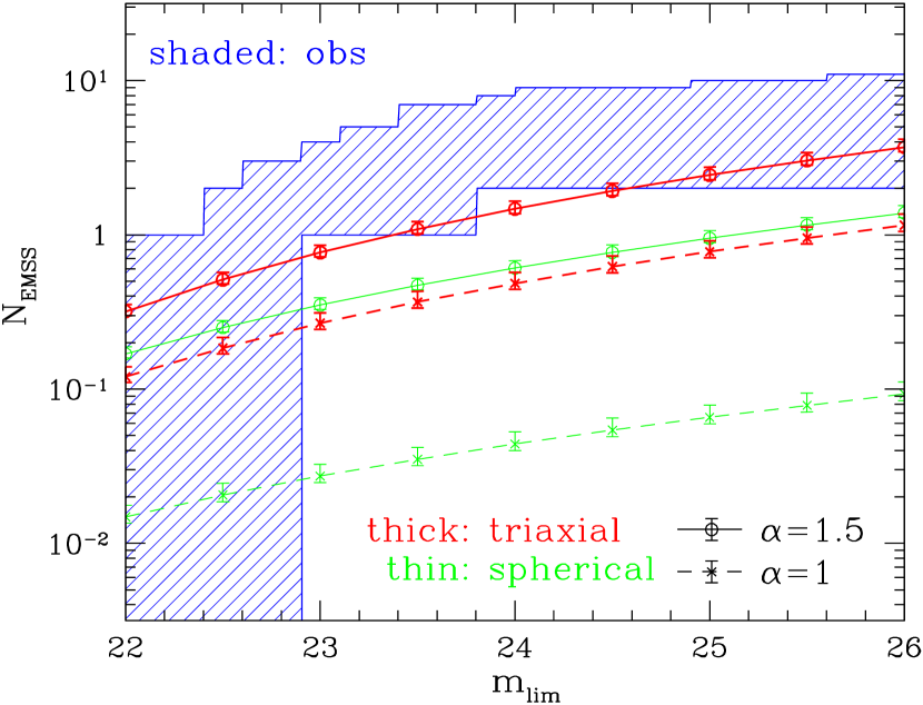
Finally let us compare our theoretical predictions with the data in detail. Our prediction of the number of arcs is the sum of equation (60) over all the 38 EMSS clusters:

$$N_{\rm EMSS}\equiv\sum^{38}_{i=1}N_{\rm arc}(M_{{\rm vir},i},z_{{\rm L},i}).$$ (67)

We also compute the error of the predicted number of arcs by propagating the mass uncertainty for each cluster (Table Arc Statistics in Triaxial Dark Matter Halos: Testing the Collisionless Cold Dark Matter Paradigm). Figure 12 shows the number of arcs in the 38 EMSS cluster sample as a function of the B-band limiting magnitude $m_{\rm lim}$. When the B-band magnitude of an arc is not available, we convert its corresponding V- or R-band magnitude into the B-band assuming typical colors of spiral galaxies at $z\sim 1$, $B-V=V-R=1$ (Fukugita et al., 1995).

The important conclusion that we draw from Figure 12 is that the triaxial model in the Lambda-dominated CDM universe with the inner slope of $\alpha=1.5$ successfully reproduces the observed number of arcs, and that the spherical model prediction with $\alpha=1$ fails by a wide margin. Both the triaxial model with $\alpha=1$ and the spherical model with $\alpha=1.5$ are marginal in a sense that the presence of substructure in the dark halo which we ignore in the current method should systematically increase our predicted number of arcs. Indeed Meneghetti, Bartelmann, & Moscardini (2003a) reported that the substructure enhances the number of arcs with $\epsilon_{\rm th}=10$ typically by a factor 2 or 3. This is exactly the amount of enhancement that is required to reconcile those two models with the observation.

We note here that the additional contribution due to galaxies inside a cluster is generally small; Flores, Maller, & Primack (2000) and Meneghetti et al. (2000) found that galaxies increase the number of arcs merely by $\sim$10%. Even a central cD galaxy produces the number of arcs by not more than $\sim$50% (Meneghetti, Bartelmann, & Moscardini, 2003b).

6 Discussion

6.1 Comparison with the previous result

Our result that the halos in a Lambda-dominated CDM universe reproduces the observed number of arcs seems inconsistent with the previous result of Bartelmann et al. (1998) who claimed that only open CDM models can reproduce the observation. One possibility to explain the apparent discrepancy is the difference of the inner profile of halos; we showed that the slope of $\alpha=1.5$ is required to reproduce the observation. This implies that N-body simulations may underestimate the real number of arcs unless they have sufficient spatial resolution. On the other hand, cluster-scale halos may indeed have a shallower inner profile (Jing & Suto, 2000). Therefore this is closely related to the well known problem of the inner slope of CDM dark matter halos (Navarro et al., 1996, 1997; Moore et al., 1999; Jing & Suto, 2000; Fukushige & Makino, 2001, 2003; Power et al., 2003), and would need further investigation. Moreover, in reality, the mass estimate for each cluster, the limiting magnitude of source galaxies, and the adopted luminosity function would also affect the prediction in a more complicated fashion, and the further quantitative comparison is not easy at this point.

Figure 13: The number of arcs in the 38 EMSS cluster sample as a function of $A_{e}$ for $m_{\rm lim}=24$. Dash-dotted line indicates the fiducial value for $A_{e}$, $A_{e}=1.1$, in a Lambda-dominated CDM model. Dotted lines suggest possible range of $A_{e}$ with taking account of the enhancement of the concentration parameter in an open CDM model (see text for details).

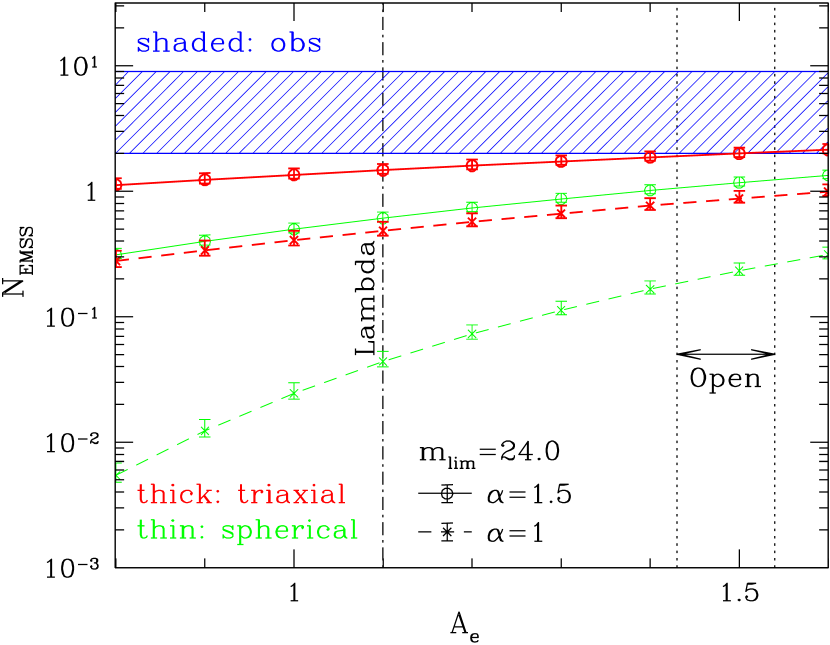
Nevertheless we can point out the general tendency that open CDM models produce more arcs than Lambda-dominated CDM models because of the larger value of the concentration parameter in the former. Thus it is unlikely that difference between open and Lambda-dominated CDM models results from the “global” effect of the cosmological parameters. In order to show this, we compute the number of arcs as a function of $A_{e}$ still assuming the Lambda-dominated CDM model. Figure 13 plots $N_{\rm EMSS}$ for $m_{\rm lim}=24$ as a function of $A_{e}$. While JS02 found $A_{e}=1.1$ in a Lambda-dominated CDM models, their fitting formula (see also Bartelmann et al., 1998) tend to predict $\sim 30-40\%$ larger concentration parameter in open CDM models. This enhancement of the concentration parameter corresponds to $A_{e}=1.43\sim 1.53$ if we still assume Lambda-dominated CDM models as a background cosmology. Thus the effect of $A_{e}$ alone increases the number of arc by $\sim 50\%-100\%$ even for triaxial cases, which is qualitatively consistent with the result of Bartelmann et al. (1998).

6.2 Required Non-sphericity of Lensing Halos

Figure 14: The number of arcs in the 38 EMSS cluster sample for fixed axis ratios of dark matter halos. The B-band limiting magnitude is set to $m_{\rm lim}=24$. Left panel plots the oblate case ($a<b=c$) while right panel is the prolate case ($a=b<c$).

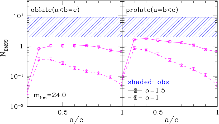
Although we showed that the triaxial halos predicted in the Lambda-dominated CDM model reproduce the observed number of arcs, the analysis employed a series of fairly complicated PDFs for the axial ratios of JS02, and it is not so clear what degree of non-sphericity for lensing halos is required to account for the observation. Thus we rather simplify the situation and consider that all halos consist of oblate ($a<b=c$) or prolate ($a=b<c$) halos with a fixed axial ratio. This is equivalent to replacing $p(a/c)$ (eq. [13]) or $p(a/b)$ (eq. [14]) by the corresponding $\delta$-functions. Figure 14 plots the result of this exercise.

The predicted number of arcs is indeed sensitive to the axis ratios of dark matter halos, and prolate halos of $a/c\lesssim 0.5$ in the $\alpha=1.5$ case reproduce the observation. This is basically consistent with the finding of JS02 for halo properties.

The reason why prolate halos tend to produce the larger number of arcs than oblate halos is explained as follows. Notice first that to keep the mass of dark matter halo invariant with the change of the axial ratio, $b_{\rm TNFW}$ should be approximately proportional to $(ab/c^{2})^{-1}$. Suppose that oblate and prolate halos are projected onto their axisymmetric direction ($x$ for oblate and $z$ for prolate). Then their lensing cross sections should scale as

$$\sigma({\rm oblate}) \propto \tilde{\sigma}((a/c)(a/c)^{-1}b_{\rm TNFW},1)=\tilde{\sigma}(b_{\rm TNFW},1),$$ (68)

$$\sigma({\rm prolate}) \propto \left(\frac{a}{c}\right)^{2}\tilde{\sigma}((a/c)^{-2}b_{\rm TNFW},1)=\left(\frac{a}{c}\right)^{2-2\delta}\tilde{\sigma}(b_{\rm TNFW},1),$$ (69)

where we assume $\tilde{\sigma}(b_{\rm TNFW},q)\propto b_{\rm TNFW}^{\delta}$. Since Figures 3 and 4 suggest $\delta\gtrsim 2$, we find that $\sigma({\rm prolate})\gg\sigma({\rm oblate})$ for $a/c<1$. If those halos are projected along the $y$-direction, on the other hand, their cross sections are almost the same:

$$\sigma({\rm oblate})\sim\sigma({\rm prolate})\propto\left(\frac{a}{c}\right)^{-\delta}\tilde{\sigma}(b_{\rm TNFW},a/c).$$ (70)

The above consideration explains the qualitative difference between oblate and prolate halos, and points out that the elongation along the line-of-sight is also important in the arc statistics as well as the asymmetry of the projected mass density.

6.3 Are Clusters Equilibrium Dark Matter Halos?

So far we have assumed the one-to-one correspondence between dark matter halos and X-ray clusters. This assumption, however, is definitely over-simplified (Suto, 2001, 2003). If “dark clusters” which are often reported from recent weak lensing analyses (Hattori et al., 1997a; Wittman et al., 2001; Miyazaki et al., 2002) are real, the one-to-one correspondence approximation may be unexpectedly inaccurate. As an extreme possibility, let us suppose that observed X-ray clusters preferentially correspond to halos in equilibrium. According to Jing (2000), such halos have generally larger concentration parameters and their scatter is small. In order to imitate this situation, we repeat the computation using $A_{e}=1.3$ and the scatter of $0.18$ (Jing 2000; JS02). We find that this modified model increases the number of arcs merely by 10%$-$20%. Thus our conclusion remains the same.

6.4 Sample Variance

Figure 15: The effect of the sample variance. The number of arcs in the 38 EMSS cluster sample is calculated, not being averaged over axis ratios, orientation, and concentration parameters, but using fixed values for each clusters. Axis ratios, orientation, and concentration parameters for each cluster are randomly chosen according to their corresponding PDFs (§2.2). We calculate 10000 realizations and plot the histogram of frequency. Averaged values are shown by arrows.

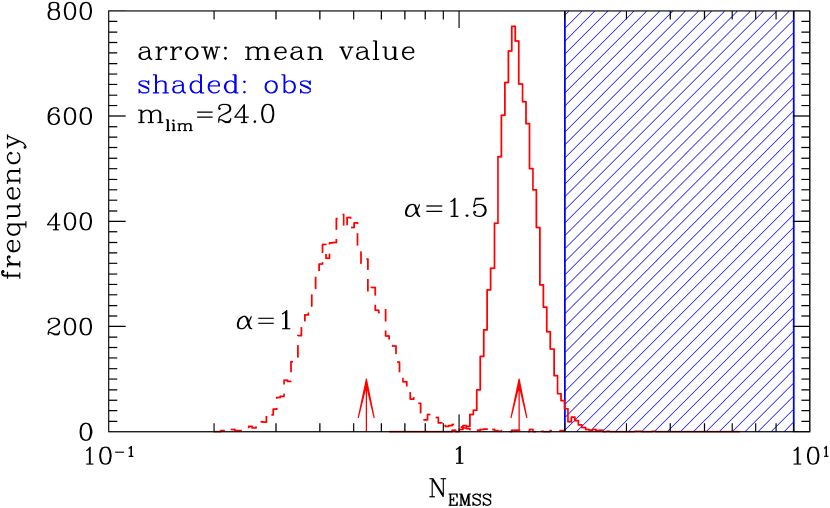
The predicted number of arcs for the EMSS cluster that we have presented so far is based on the averaged cross section. This is a reasonably good approximation in the situation that the number of sample clusters is large enough, but in the current sample, its validity is not clear. To examine the sample variance, we re-compute the number of arcs in the 38 EMSS cluster sample without using the average statistics. Instead, we first randomly choose values of the axis ratios, the orientation angles, and the concentration parameters for each cluster according to their corresponding PDFs (§2.2). Then we sum up the number of arcs for the entire cluster sample. We repeat the procedure 10000 times each for $\alpha=1$ and 1.5, and construct a distribution function of $N_{\rm EMSS}$ as plotted in Figure 15. The resulting 1$\sigma$ sample variance is $\sim$30% for $\alpha=1$ and $\sim$15% for $\alpha=1.5$. Therefore we confirm that the effect of the sample variance does not change our overall conclusion.

7 Conclusions

We have presented a semi-analytic method to predict the number of lensed arcs, for the first time taking proper account of the triaxiality of lensing halos. We found that Lambda-dominated CDM models successfully reproduce the observed number of arcs of X-ray-selected clusters (Luppino et al., 1999) if the inner slope of the density profile is close to $\alpha=1.5$. Since the spherical models significantly underestimate the expected number of arcs, we conclude that the observed number of arcs indeed requires the non-sphericity of the lensing halos. In fact, the number of arcs is sensitive to the axis ratios of those halos, and the non-sphericity that reproduces the observed number corresponds to the minor to major axis ratios of $\sim 0.5$. This value is perfectly consistent with the findings of JS02 in the Lambda-dominated CDM models. In this sense, we may even argue that the arc statistics lend strong support for the collisionless CDM paradigm at the mass scale of clusters. As discussed in Meneghetti et al. (2001), self-interacting dark matter models (Spergel & Steinhardt, 2000) for instance, are inconsistent with the observed number of arcs not only because they erase the central cusp but because they produce much rounder dark matter halos (Yoshida et al., 2000a, b). Since we have exhibited that even the current arc surveys have a great impact in testing the collisionless CDM paradigm, larger surveys with well-controlled systematics in near future will unveil the nature of dark matter more precisely.

Note added – In the published version, we used an incorrect PDF of the angle $\theta$ (eq. [47]). In this version of the preprint, we used the correct PDF and replaced all related figures to the correct ones. In these new plots, however, the number of arcs in the triaxial dark matter halo model becomes smaller only by $\sim 30$%, so this does not affect the conclusion of the paper.

Table 1: B-band luminosity functions of source galaxies used in this paper.

Name	Model	$z$ Range	$\alpha_{\rm s}$	$M^{*}_{AB}-5\log h$	$\phi^{*}[h^{3}{\rm Mpc^{-3}]}$	Ref.
HDF1	Lambda	$0.00$ - $0.50$	$-1.19$	$-20.26$	$2.5\times 10^{-2}$	1
		$0.50$ - $0.75$	$-1.19$	$-19.97$	$2.9\times 10^{-2}$
		$0.75$ - $1.25$	$-1.25$	$-20.61$	$1.2\times 10^{-2}$
HDF2	EdS	$0.00$ - $0.50$	$-1.40$	$-21.20$	$9.0\times 10^{-3}$	2
		$0.50$ - $1.00$	$-1.30$	$-19.90$	$4.2\times 10^{-2}$
		$1.00$ - $1.25$	$-1.60$	$-22.10$	$6.0\times 10^{-3}$
SDF	EdS	$0.00$ - $1.00$	$-1.07$	$-19.78$	$4.2\times 10^{-2}$	3
		$1.00$ - $1.25$	$-0.92$	$-20.13$	$4.3\times 10^{-2}$
CFRS	EdS	$0.00$ - $0.50$	$-1.03$	$-19.53$	$2.7\times 10^{-2}$	4
		$0.50$ - $0.75$	$-0.50$	$-19.32$	$6.2\times 10^{-2}$
		$0.75$ - $1.00$	$-1.28$	$-19.73$	$5.4\times 10^{-2}$
		$1.00$ - $1.25$	$-2.50$	$-21.36$	$9.6\times 10^{-4}$

References. — (1) Poli et al. 2001; (3) Sawicki et al. 1997; (3) Kashikawa et al. 2003; (4) Lilly et al. 1995

Table 2: Properties of clusters in the $38$ EMSS distant cluster sample.

		$L_{X}$(EdS)	$L_{X}$(Lambda)	$T_{X}$	$M_{\rm vir}$
Name	$z_{\rm L}$	[$10^{44}{\rm erg\,s^{-1}}$]	[$10^{44}{\rm erg\,s^{-1}}$]	[${\rm keV}$]	[$10^{14}h^{-1}M_{\odot}$]	Ref.
MS 0011.7$+$0837	$0.163$	$3.77$	$2.24$	$4.79^{+0.48}_{-0.44}$	$3.89^{+0.72}_{-0.66}$	1
MS 0015.9$+$1609	$0.546$	$14.64$	$11.03$	$8.92^{+0.57}_{-0.56}$	$12.30^{+1.46}_{-1.43}$	1, 2
MS 0302.5$+$1717	$0.425$	$2.88$	$2.04$	$4.62^{+0.45}_{-0.41}$	$3.64^{+0.66}_{-0.60}$	1
MS 0302.7$+$1658	$0.426$	$5.04$	$3.57$	$4.35^{+0.80}_{-0.64}$	$3.25^{+1.11}_{-0.89}$	1, 2
MS 0353.6$-$3642	$0.320$	$5.24$	$3.48$	$6.46^{+0.98}_{-0.80}$	$6.77^{+1.90}_{-1.55}$	1, 2
MS 0433.9$+$0957	$0.159$	$4.34$	$2.57$	$5.04^{+0.53}_{-0.48}$	$4.27^{+0.83}_{-0.75}$	1
MS 0440.5$+$0204	$0.190$	$4.01$	$2.43$	$5.30^{+0.60}_{-0.40}$	$4.69^{+0.98}_{-0.66}$	1, 3
MS 0451.5$+$0250	$0.202$	$6.98$	$4.27$	$8.60^{+0.50}_{-0.50}$	$11.50^{+1.24}_{-1.24}$	1, 3
MS 0451.6$-$0305	$0.539$	$19.98$	$15.00$	$10.27^{+0.85}_{-0.80}$	$15.97^{+2.45}_{-2.30}$	1, 2
MS 0735.6$+$7421	$0.216$	$6.12$	$3.79$	$5.85^{+0.68}_{-0.61}$	$5.63^{+1.21}_{-1.09}$	1
MS 0811.6$+$6301	$0.312$	$2.10$	$1.40$	$4.87^{+0.95}_{-0.63}$	$4.01^{+1.45}_{-0.96}$	1, 2
MS 0839.8$+$2938	$0.194$	$5.35$	$3.25$	$4.20^{+0.20}_{-0.20}$	$3.05^{+0.27}_{-0.27}$	1, 3
MS 0906.5$+$1110	$0.180$	$5.77$	$3.47$	$5.65^{+0.64}_{-0.58}$	$5.28^{+1.11}_{-1.00}$	1
MS 1006.0$+$1201	$0.221$	$4.82$	$2.99$	$5.34^{+0.58}_{-0.52}$	$4.76^{+0.96}_{-0.86}$	1
MS 1008.1$-$1224	$0.301$	$4.49$	$2.95$	$8.21^{+1.15}_{-1.05}$	$10.55^{+2.74}_{-2.50}$	1, 2
MS 1054.5$-$0321	$0.823$	$9.28$	$7.79$	$10.4^{+1.00}_{-1.00}$	$16.35^{+2.91}_{-2.91}$	1, 4
MS 1137.5$+$6625	$0.782$	$7.56$	$6.26$	$5.70^{+0.80}_{-0.60}$	$5.37^{+1.40}_{-1.05}$	1, 5
MS 1147.3$+$1103	$0.303$	$2.30$	$1.51$	$5.96^{+0.99}_{-0.69}$	$5.83^{+1.79}_{-1.25}$	1, 2
MS 1201.5$+$2824	$0.167$	$2.03$	$1.21$	$3.78^{+0.34}_{-0.32}$	$2.51^{+0.42}_{-0.39}$	1
MS 1208.7$+$3928	$0.340$	$2.03$	$1.37$	$3.97^{+0.36}_{-0.33}$	$2.75^{+0.46}_{-0.42}$	1
MS 1224.7$+$2007	$0.327$	$4.61$	$3.08$	$4.09^{+0.65}_{-0.52}$	$2.90^{+0.85}_{-0.68}$	1, 2
MS 1231.3$+$1542	$0.238$	$2.88$	$1.81$	$4.41^{+0.42}_{-0.39}$	$3.34^{+0.59}_{-0.55}$	1
MS 1241.5$+$1710	$0.549$	$10.70$	$8.07$	$6.09^{+1.38}_{-1.14}$	$6.07^{+2.55}_{-2.10}$	1, 2
MS 1244.2$+$7114	$0.225$	$3.84$	$2.39$	$4.90^{+0.50}_{-0.46}$	$4.06^{+0.77}_{-0.71}$	1
MS 1253.9$+$0456	$0.230$	$3.14$	$1.96$	$4.55^{+0.44}_{-0.40}$	$3.54^{+0.63}_{-0.58}$	1
MS 1358.4$+$6245	$0.327$	$10.62$	$7.09$	$7.50^{+4.30}_{-0.91}$	$8.93^{+9.48}_{-2.01}$	1, 2, 6
MS 1426.4$+$0158	$0.320$	$3.71$	$2.47$	$6.38^{+0.98}_{-1.20}$	$6.62^{+1.88}_{-2.30}$	1, 2
MS 1455.0$+$2232	$0.259$	$16.03$	$10.23$	$5.60^{+1.88}_{-1.15}$	$5.20^{+3.23}_{-1.98}$	1, 3, 6
MS 1512.4$+$3647	$0.372$	$4.81$	$3.30$	$3.39^{+0.40}_{-0.35}$	$2.05^{+0.45}_{-0.39}$	1, 2
MS 1546.8$+$1132	$0.226$	$2.94$	$1.83$	$4.43^{+0.43}_{-0.39}$	$3.37^{+0.61}_{-0.55}$	1
MS 1618.9$+$2552	$0.161$	$2.24$	$1.33$	$3.92^{+0.36}_{-0.33}$	$2.68^{+0.46}_{-0.42}$	1
MS 1621.5$+$2640	$0.426$	$4.55$	$3.22$	$6.59^{+0.92}_{-0.81}$	$7.02^{+1.82}_{-1.60}$	1, 2
MS 1910.5$+$6736	$0.246$	$4.39$	$2.78$	$5.20^{+0.55}_{-0.50}$	$4.53^{+0.89}_{-0.81}$	1
MS 2053.7$-$0449	$0.583$	$5.78$	$4.43$	$8.14^{+3.68}_{-2.15}$	$10.39^{+8.70}_{-5.08}$	1, 2
MS 2137.3$-$2353	$0.313$	$15.62$	$10.34$	$5.20^{+1.09}_{-0.42}$	$4.53^{+1.76}_{-0.68}$	1, 2, 6
MS 2255.7$+$2039	$0.288$	$2.04$	$1.33$	$3.92^{+0.36}_{-0.33}$	$2.68^{+0.46}_{-0.42}$	1
MS 2301.3$+$1506	$0.247$	$3.29$	$2.08$	$4.65^{+0.46}_{-0.42}$	$3.68^{+0.67}_{-0.62}$	1
MS 2318.7$-$2328	$0.187$	$6.84$	$4.14$	$6.05^{+0.73}_{-0.65}$	$6.00^{+1.34}_{-1.19}$	1

Note. — Errors are at $68$% confidence limit.

References. — (1) Luppino et al. 1999; (2) Novicki, Sornig, & Henry 2002; (3) Mushotzky & Scharf 1997; (4) Jeltema et al. 2001; (5) Borgani et al. 2001; (6) Allen & Fabian 1998

Table 3: Giant arcs ($l/w>10$) in the $38$ EMSS distant cluster sample.

Cluster	$z_{\rm L}$	Arc	$z_{\rm S}$	$l/w$	$m_{\rm arc}$	Notes	Ref.
MS 0302.7$+$1658	$0.426$	A1	$\sim 0.8$	$>18$	$B=23.8$	$\cdots$	1, 2
		A1W	$\cdots$	$>12$	$B=24.9$	$\cdots$
MS 0440.5$+$0204	$0.190$	A1	$0.532$	$>10$	$B=22.9$	$\cdots$	1, 3, 4
		A3	$\cdots$	$>20$	$B=24.0$	$\cdots$
MS 0451.6$-$0305	$0.539$	A1	$\cdots$	$10$	$V=24.6$	$\cdots$	1
MS 1006.0$+$1201	$0.221$	A2$+$A3	$\cdots$	$>20$	$V<22.1$	Candidate	1, 5
		A4	$\cdots$	$12.9$	$V=21.4$	Candidate
MS 1008.1$-$1224	$0.301$	A2	$\cdots$	$10.0$	$B=23.4$	Candidate	1
MS 1358.4$+$6245	$0.328$	A1	$4.92$	$>21$	$\cdots$	$\cdots$	1, 6
MS 1621.5$+$2640	$0.426$	A1	$\cdots$	$>18$	$B=23.1$	$\cdots$	1, 7
MS 1910.5$+$6736	$0.246$	A1	$\cdots$	$10.5$	$R=20.6$	Candidate	1, 5
MS 2053.7$-$0449	$0.583$	AB	$\cdots$	$>22$	$V=22.4$	$\cdots$	1, 7
MS 2137.3$-$2353	$0.313$	A1	$1.501$	$18.1$	$B=22.0$	$\cdots$	1, 8, 9, 10

References. — (1) Luppino et al. 1999; (2) Mathez et al. 1992; (3) Luppino et al. 1993; (4) Gioia et al. 1998 (5); Le Févre et al. 1994; (6) Franx et al. 1997; (7) Luppino & Gioia 1992; (8) Fort et al. 1992; (9) Hammer et al. 1997; (10) Sand et al. 2002

References

- Allen & Fabian (1998) Allen, S. W. & Fabian, A. C. 1998, MNRAS, 297, L57
- Bartelmann (1995) Bartelmann, M. 1995, A&A, 299, 11
- Bartelmann (1996) Bartelmann, M. 1996, A&A, 313, 697
- Bartelmann et al. (1998) Bartelmann, M., Huss, A., Colberg, J. M., Jenkins, A., & Pearce, F. R. 1998, A&A, 330, 1
- Bartelmann et al. (2003) Bartelmann, M., Meneghetti, M., Perrotta, F., Baccigalupi, C., & Moscardini, L. 2003, A&A, 409, 449
- Bartelmann et al. (1995) Bartelmann, M., Steinmetz, M., & Weiss, A. 1995, A&A, 297, 1
- Bartelmann & Weiss (1994) Bartelmann, M., & Weiss, A. 1994, A&A, 287, 1
- Binney (1985) Binney, J. 1985, MNRAS, 212, 767
- Borgani et al. (2001) Borgani, S., et al. 2001, ApJ, 561, 13
- Clowe & Schneider (2001) Clowe, D., & Schneider, P. 2001, A&A, 379, 384
- Clowe & Schneider (2002) Clowe, D., & Schneider, P. 2002, A&A, 395, 385
- Cooray (1999) Cooray, A. R. 1999, ApJ, 524, 504
- Finoguenov et al. (2001) Finoguenov, A., Reiprich, T. H., & Böhringer, H. 2001, A&A, 368, 749
- Flores et al. (2000) Flores, R. A., Maller, A. H., & Primack, J. R. 2000, ApJ, 535, 555
- Fort et al. (1992) Fort, B., Le Févre, O., Hammer, F., & Cailloux, M. 1992, ApJ, 399, L125
- Franx et al. (1997) Franx, M., Illingworth, G. D., Kelson, D. D., van Dokkum, P. G., & Tran, K. 1997, ApJ, 486, L75
- Fukugita et al. (1995) Fukugita, M., Shimasaku, K., & Ichikawa, T. 1995, PASP, 107, 945
- Fukushige & Makino (2001) Fukushige, T., & Makino, J. 2001, ApJ, 557, 533
- Fukushige & Makino (2003) Fukushige, T., & Makino, J. 2003, ApJ, 588, 674
- Gavazzi et al. (2003) Gavazzi, R., Fort, B., Mellier, Y., Pello, R., & Dantel-Fort, M. 2003, A&A, 403, 11
- Gioia et al. (1998) Gioia, I. M., Shaya, E. J., Le Févre, O., Falco, E. E., Luppino, G. A., & Hammer, F. 1998, ApJ, 497, 573
- Gladders et al. (2003) Gladders, M. D., Hoekstra, H., Yee, H. K. C., Hall, P. B., & Barrientos, L. F. 2003, ApJ, 593, 48
- Golse et al. (2002) Golse, G., Kneib, J.-P., & Soucail, G. 2002, A&A, 387, 788
- Hamana & Futamase (1997) Hamana, T., & Futamase, T. 1997, MNRAS, 286, L7
- Hammer et al. (1997) Hammer, F., Gioia, I. M., Shaya, E. J., Teyssandier, P., Le Févre, O., & Luppino, G. A. 1997, ApJ, 491, 477
- Hattori et al. (1997a) Hattori, M., et al. 1997a, Nature, 388, 146
- Hattori et al. (1997b) Hattori, M., Watanabe, K., & Yamashita, K. 1997b, A&A, 319, 764
- Ikebe et al. (2002) Ikebe, Y., Reiprich, T. H., Böhringer, H., Tanaka, Y., & Kitayama, T. 2002, A&A, 383, 773
- Jeltema et al. (2001) Jeltema, T. E., Canizares, C. R., Bautz, M. W., Malm, M. R., Donahue, M., & Garmire, G. P. 2001, ApJ, 562, 124
- Jing (2000) Jing, Y. P. 2000, ApJ, 535, 30
- Jing & Suto (2000) Jing, Y. P., & Suto, Y. 2000, ApJ, 529, L69
- Jing & Suto (2002) Jing, Y. P., & Suto, Y. 2002, ApJ, 574, 538 (JS02)
- Kashikawa et al. (2003) Kashikawa, N., et al. 2003, AJ, 125, 53
- Keeton (2001a) Keeton, C. R. 2001a, preprint (astro-ph/0102341)
- Keeton (2001b) Keeton, C. R. 2001b, ApJ, 562, 160
- Keeton & Madau (2001) Keeton, C. R., & Madau, P. 2001, ApJ, 549, L25
- King & Ellis (1985) King, C. R., & Ellis, R. S. 1985, ApJ, 288, 456
- Lambas et al. (1992) Lambas, D. G., Maddox, S. J., & Loveday, J. 1992, MNRAS, 258, 404
- Le Févre et al. (1994) Le Févre, O., Hammer, F., Angonin, M. C., Gioia, I. M., & Luppino, G. A. 1994, ApJ, 422, L5
- Li & Ostriker (2003) Li, L.-X., & Ostriker, J. P. 2003, ApJ, 595, 603
- Lilly et al. (1995) Lilly, S. J., Tresse, L., Hammer, F., Crampton, D., & Le Févre, O. 1995, ApJ, 455, 108
- Luppino & Gioia (1992) Luppino, G. A. & Gioia, I. M. 1992, A&A, 265, L9
- Luppino et al. (1993) Luppino, G. A., Gioia, I. M., Annis, J., Le Févre, O., & Hammer, F. 1993, ApJ, 416, 444
- Luppino et al. (1999) Luppino, G. A., Gioia, I. M., Hammer, F., Le Févre, O., & Annis, J. A. 1999, A&AS, 136, 117
- Lynds & Petrosian (1986) Lynds, R., & Petrosian, V. 1986, BAAS, 18, 1014
- Maoz et al. (1997) Maoz, D., Rix, H.-W., Gal-Yam, A., Gould, A. 1997, ApJ, 486, 75
- Mathez et al. (1992) Mathez, G., Fort, B., Mellier, Y., Picat, J.-P., & Soucail, G. 1992, A&A, 256, 343
- Meneghetti et al. (2000) Meneghetti, M., Bolzonella, M., Bartelmann, M., Moscardini, L., & Tormen, G. 2000, MNRAS, 314, 338
- Meneghetti et al. (2001) Meneghetti, M., Yoshida, N., Bartelmann, M., Moscardini, L., Springel, V., Tormen, G., & White S. D. M. 2001, MNRAS, 325, 435
- Meneghetti et al. (2003a) Meneghetti, M., Bartelmann, M., & Moscardini, L. 2003a, MNRAS, 340, 105
- Meneghetti et al. (2003b) Meneghetti, M., Bartelmann, M., & Moscardini, L. 2003b, MNRAS, 346, 67
- Miralda-Escudé (1993a) Miralda-Escudé, J. 1993a, ApJ, 403, 497
- Miralda-Escudé (1993b) Miralda-Escudé, J. 1993b, ApJ, 403, 509
- Miralda-Escudé (1995) Miralda-Escudé, J. 1995, ApJ, 438, 514
- Miralda-Escudé (2002) Miralda-Escudé, J. 2002, ApJ, 564, 60
- Miyazaki et al. (2002) Miyazaki, S., et al. 2002, ApJ, 580, L97
- Molikawa & Hattori (2001) Molikawa, K., & Hattori, M. 2001, ApJ, 559, 544
- Molikawa et al. (1999) Molikawa, K., Hattori, M., Kneib, J. P., & Yamashita, K. 1999, A&A, 351, 413
- Moore et al. (1999) Moore, B., Quinn, T., Governato, F., Stadel, J., & Lake, G. 1999, MNRAS, 310, 1147
- Mushotzky & Scharf (1997) Mushotzky, R. F. & Scharf, C. A. 1997, ApJ, 482, L13
- Navarro et al. (1996) Navarro, J. F., Frenk, C. S., & White, S. D. M. 1996, ApJ, 462, 563
- Navarro et al. (1997) Navarro, J. F., Frenk, C. S., & White, S. D. M. 1997, ApJ, 490, 493
- Novicki et al. (2002) Novicki, M. C., Sornig, M., & Henry, J. P. 2002, AJ, 124, 2413
- Oguri (2002a) Oguri, M. 2002a, ApJ, 573, 51
- Oguri (2002b) Oguri, M. 2002b, ApJ, 580, 2
- Oguri (2003) Oguri, M. 2003, MNRAS, 339, L23
- Oguri et al. (2001) Oguri, M., Taruya, A., & Suto, Y. 2001, ApJ, 559, 572
- Poli et al. (2001) Poli, F., Menci, N., Giallongo, E., Fontana, A., Cristiani, S., & D’Odorico, S. 2001, ApJ, 551, L45
- Power et al. (2003) Power, C., Navarro, J. F., Jenkins, A., Frenk, C. S., White, S. D. M., Springel, V., Stadel, J., & Quinn, T. 2002, MNRAS, 338, 14
- Sand et al. (2002) Sand, D. J., Treu, T., & Ellis, R. S. 2002, ApJ, 574, L129
- Sawicki et al. (1997) Sawicki, M. J., Lin, H., & Yee, H. K. C. 1997, AJ, 113, 1
- Schneider et al. (1992) Schneider, P., Ehlers, J., & Falco, E. E. 1992, Gravitational Lenses (New York: Springer)
- Schramm (1990) Schramm, T. 1990, A&A, 231, 19
- Sereno (2002) Sereno, M. 2002, A&A, 393, 757
- Shimizu et al. (2003) Shimizu, M., Kitayama, T., Sasaki, S., & Suto, Y. 2003, ApJ, 590, 197
- Smith et al. (2001) Smith, G. P., Kneib, J., Ebeling, H., Czoske, O., & Smail, I. 2001, ApJ, 552, 493
- Soucail et al. (1987) Soucail, G., Fort, B., Mellier, Y., & Picat, J. P. 1987, A&A, 172, L14
- Spergel & Steinhardt (2000) Spergel, D. N., & Steinhardt P. J. 2000, Phys. Rev. Lett., 84, 3760
- Spergel et al. (2003) Spergel, D. N., et al. 2003, ApJS, 148, 175
- Suto (2001) Suto, Y. 2001, in the proceedings of “AMiBA 2001: High-z Clusters, Missing Baryons, and CMB Polarization”, eds. L.-W. Chen, C.-P. Ma, K.-W. Ng & U.-L. Pen (San Francisco: ASP), 195 (astro-ph/0110073)
- Suto (2003) Suto, Y. 2003, in the proceedings of “Matter and Energy in Clusters of Galaxies”, eds. S. Bowyer & C.-Y. Hwang (San Francisco: ASP), 370 (astro-ph/0207202)
- Turner (1980) Turner, E. L. 1980, ApJ, 242, L135
- Turner et al. (1984) Turner, E. L., Ostriker, J. P., & Gott, J. R. 1984, ApJ, 284, 1
- Wambsganss et al. (2003) Wambsganss, J., Bode, P., & Ostriker, J. P. 2003, ApJ, submitted (astro-ph/0306088)
- Williams et al. (1999) Williams, L. L. R., Navarro, J. F., & Bartelmann, M. 1999, ApJ, 527, 535
- Wittman et al. (2001) Wittman, D., Tyson, J. A., Margoniner, V. E., Cohen, J. G., & Dell’Antonio, I. P. 2001, ApJ, 557, L89
- Wu & Hammer (1993) Wu, X.-P., & Hammer, F. 1993, MNRAS, 262, 187
- Wu & Mao (1996) Wu, X.-P., & Mao, S. 1996, ApJ, 463, 404
- Yoshida et al. (2000a) Yoshida, N., Springel, V., White, S. D. M., & Tormen, G. 2000a, ApJ, 535, L103
- Yoshida et al. (2000b) Yoshida, N., Springel, V., White, S. D. M., & Tormen, G. 2000b, ApJ, 544, L87
- Zaritsky & Gonzalez (2003) Zaritsky, D. & Gonzalez, A. H. 2003, ApJ, 584, 691