The 2001 April Burst Activation of SGR 1900+14: X-ray afterglow emission

Abstract

After nearly two years of quiescence, the soft gamma-ray repeater SGR 1900+14 again became burst-active on April 18 2001, when it emitted a large flare, preceded by few weak and soft short bursts. After having detected the X and gamma prompt emission of the flare, BeppoSAX pointed its narrow field X-ray telescopes to the source in less than 8 hours. In this paper we present an analysis of the data from this and from a subsequent BeppoSAX observation, as well as from a set of RossiXTE observations. Our data show the detection of an X-ray afterglow from the source, most likely related to the large hard X-ray flare. In fact, the persistent flux from the source, in 2-10 keV, was initially found at a level $\sim$5 times higher than the usual value. Assuming an underlying persistent (constant) emission, the decay of the excess flux can be reasonably well described by a t^-0.9 law. A temporal feature - a $\sim$half a day long bump - is observed in the decay light curve approximately one day after the burst onset. This feature is unprecedented in SGR afterglows. We discuss our results in the context of previous observations of this source and derive implications for the physics of these objects.

1 Introduction

Soft gamma-ray repeaters (SGRs) are a small class of high energy transients, comprising four confirmed members and a candidate one (see e.g. Hurley 2001a for a recent observational review). These sources usually manifest themselves through the emission of short (few hundreds of milliseconds) bursts of hard-X/gamma-rays recurring on variable timescales, from minutes to days to years. All of the confirmed SGRs have been identified as steady X-ray emitters (e.g., Hurley 2001a, and references therein) with luminosity in the range of 10³³-10³⁶ erg s^-1 (2-10 keV). The X-ray radiation emitted by two of the SGRs, SGR 1806-20 and SGR 1900+14, is coherently modulated with periods of $\sim$7.5 and $\sim$5.2 s, respectively Kouveliotou et al. (1998); Hurley et al. 1999a ; both sources show a secular spindown of $\sim$10^-10 s s^-1 (e.g., Mereghetti et al. 2000, Kouveliotou et al. 1998, Hurley et al. 1999a, Woods et al. 1999a). SGR 0526-66 exhibited coherent 8-s pulsations during the decaying part of its famous 1979 March 5th giant flare Mazets et al. (1979). These pulsations were also seen during recent Chandra observations of the source, albeit at a lesser statistical significance Kulkarni et al. (2003). Finally, no periodicity was found in the X-ray flux of SGR 1627-41 Woods et al. 1999b ; Hurley et al. (2000).

One of the dramatic manifestation of the SGR sources are their giant flares. Two sources have emitted such events so far: SGR 0526-66 (1979 March 5, Mazets et al. 1979), and SGR 1900+14 (1998 August 27, Hurley et al. 1999b, Feroci et al. 1999, Mazets et al. 1999a). These events are strikingly similar (see, e.g., Mazets ey al. 1999a and Feroci et al. 2001a), very different from the more frequent short recurrent bursts. In summary, both SGR giant flares have light curves consisting of an initial short and very hard spike followed by a much longer (several hundreds of seconds) tail, modulated with the spin period of the neutron star.

The most important properties that distinguish these “giant” flares from the short recurrent bursts are their peak fluxes ($\sim$10^-3-10^-2 vs 10^-6-10^-5 ergs cm^-2 s^-1 in the short bursts), their total energy ($>$10⁴⁴ ergs vs $\lesssim$10⁴¹ ergs of the short bursts), their duration ($\sim$300 s vs. few hundreds of milliseconds), their periodically modulated time profile and the hard component in their energy spectrum (in contrast to the thermal spectrum of the short bursts), particularly in the very hard short spike emitted at the beginning of the event.

Until recently, therefore, the distribution of SGR outbursts appeared to be bimodal, comprising smaller outbursts and giant flares. Recently, an event with ’intermediate’ fluence and duration of $\sim$0.5 s was detected from SGR 1627-41 (Mazets et al. 1999b, see also Kouveliotou et al. 2001 for a general discussion on the distribution of properties of SGR outbursts). In addition, on 2001 April 18, 07:55:12 UT, after almost two years of burst-quiescence, SGR 1900+14 emitted a ‘brand new’ type of ‘intermediate’ outburst that was detected by the BeppoSAX Gamma Ray Burst Monitor Guidorzi et al. (2001). The event had the intermediate duration of $\sim$40 s, its light curve did not show any initial hard spike, and was clearly spin-modulated. Also the energetics appeared to be intermediate in the 40-700 keV energy range, with a peak flux of $\sim$10^-5 erg cm^-2 s^-1 and a fluence of $\sim 1.5\times 10^{-4}$ erg cm^-2 Guidorzi et al. (2003), corresponding (for isotropic emission at 10 kpc) to a peak luminosity of $\sim 1.3\times 10^{41}$ erg s^-1 and a total emitted energy of $\sim 1.9\times 10^{42}$ ergs. Contrary to any large outburst from SGRs observed in the past, this event was also observed at X-rays (2-26 keV) with the BeppoSAX Wide Field Cameras, that also detected three weak short bursts preceding the burst itself Feroci et al. 2001b . Unfortunately, the extreme brightness at X-rays activated the self-protective automatic shutdown of the WFC instrument after only 3 s, when a count rate of about 3$\times 10^{4}$ count s^-1 was reached. The same event was detected by the gamma-ray burst detector onboard Ulysses and by the Konus-Wind experiment. The triangulation by the Third Interplanetary Network provided an annulus consistent with the position of SGR 1900+14 Hurley et al. 2001b .

We present here observations carried out with the BeppoSAX Narrow Field Instruments (NFI, Boella et al. 1997) and the Proportional Counters Array (PCA, Jahoda et al. 1996) onboard the Rossi X-ray Timing Exporer (RXTE) soon after the April 18 event. These observations started only $\sim$8 hours after the flare, enabling us to detect an X-ray afterglow fading into quiescence after a few days. We discuss in this paper the temporal behaviour of the X-ray flux from this source. A companion paper discusses the X-ray pulse properties and timing analyses Woods et al. (2003) resulting from the same set of observations.

2 Observations and Data Analysis

2.1 BeppoSAX NFI

The detection and localization of the intermediate flare by the BeppoSAX Gamma Ray Burst Monitor and Wide Field Camera unit #1 prompted a follow-up observation with the BeppoSAX NFI, as a part of our ongoing Target of Opportunity program for active Soft Gamma-ray Repeaters. Thanks to a remarkable effort of the BeppoSAX team, the first observation started within less than 7.5 hours after the flare, namely on 18 April 2001 at 15:10 UT, and ended on 19 April 2001, at 19:38 UT, resulting in net exposure times of 46.2 and 20.4 ks for the MECS and the LECS, respectively. A second pointing started on 29 April 2001 at 20:34 UT and ended on 1 May 2001 at 08:25 UT, resulting in net exposure times of 57.2 and 23.4 ks on the MECS and the LECS, respectively.

We analysed the data from the LECS and MECS instruments starting from the cleaned event files provided by the BeppoSAX Science Data Center. The photons detected in the MECS during the first pointing (April 18) were extracted in a circular area of 4^′ radius. Given the low galactic latitude of this source, we estimated the local background from an annulus concentric with the source extraction region, of inner/outer radii of 6^′ and 9^′, respectively.

Further, we extracted a light curve of the MECS count rate, with a bin size of 1 s, from which we clearly see a large number of bursts of different intensity and duration from the source. To study the properties of the persistent emission of the source, we cleaned the event list from these bursts by applying an intensity filter between 0 and 3 counts s^-1 (the average source count rate is about 0.36 counts s^-1). This ‘cleaning’ procedure removed photons from about 70 bursts from the photon list and left a net integration time of 46.1 ks. A plot of the MECS light curve before and after this procedure is shown in Fig. 1. The analysis of these bursts will be presented elsewhere.

Figure 1: Light curve of the April 18 BeppoSAX/MECS observation before (left hand side) and after (right hand side) the removal of the bursts (see text for details). The bin size is 1 s.

The same procedures were applied to the LECS data using again extraction regions of 4^′ radius and an annulus of 9^′ and 12^′ inner/outer radius, respectively. Due to the smaller exposure time, the LECS missed several of the bursts observed with the MECS. Only 10 bursts were removed from its light curve, leaving a net exposure time of 20.4 ks.

In order to convert the count rates into physical units, we performed a simultaneous spectral fit combining the LECS (0.5-4.0 keV) and MECS (1.6-10.0 keV) data. Adopting a simple power law with photoelectric absorption we find a satisfactory fit, with reduced $\chi^{2}$=0.86 (91 degrees of freedom) and the following spectral parameters: photon index $\Gamma$ = (2.57$\pm$0.08) and N_H = (4.41$\pm$0.25)$\times 10^{22}$ cm^-2, resulting in an unabsorbed flux of 3.4$\times 10^{-11}$ erg cm^-2 s^-1 (2-10 keV). (Uncertainties on fit parameters are given at 90% confidence level, whereas on data points they are 1-$\sigma$.)

The burst-cleaned MECS photon list was then used to extract a light curve. We choose time bins of 10⁴ s to derive the light curve that, converted to $cgs$ units using the counts to energy conversion obtained from the above time-averaged spectrum, is plotted in Fig. 2 (full blue triangles, on the left hand side). In order to check whether our counts-to-flux conversion procedure could be significantly affected by any intra-observation spectral variability, we computed a time-resolved hardness ratio between the MECS energy ranges 4-10 keV and 1.6-4 keV (Fig. 2, bottom panel). Indeed, we observe a general softening trend of the spectrum across the observation but the spectral variation does not affect the counts-to-flux conversion to more than a few percent, as also verified through time-resolved spectra (see Mereghetti et al. 2003 for details). Therefore, for simplicity we decided to use a single conversion factor for the entire observation.

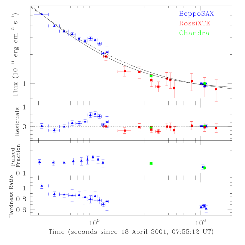
Figure 2: Top Panel: Temporal behaviour of the X-ray (2-10 keV) flux from SGR 1900+14 in the aftermath of the April 18 2001 flare, as observed with the BeppoSAX NFI, Chandra ACIS and the RossiXTE PCA, together with the best-fit curves (see text for details) with a constant plus a power law decay, including (dashed line) or excluding (solid line) the data points in the bump. Second Panel: Flux residuals from the fit performed excluding the data points in the bump. The horizontal dotted line indicates the zero. Third Panel: Light curve of the pulsed fraction during the two BeppoSAX observations, as observed with the MECS, and during the two Chandra ACIS observations (Woods et al. 2003). Bottom Panel: Hardness ratio of the two BeppoSAX observations, between the MECS energy ranges 4-10 keV and 1.6-4 keV. (Uncertainties on all data points are 1-$\sigma$.)

The same procedures were also applied to the data of the second NFI observation (April 29). However, during this observation we only detected a single burst, thus the net exposure times of the cleaned data were 23 ks for the LECS and 57 ks for the MECS. The energy spectra from this observation cannot be fit with an absorbed single power law. The resulting reduced $\chi^{2}$ of this fit is 1.34 (72 degrees of freedom). Motivated by the general knowledge on the energy spectra from these sources (e.g., Woods et al. 1999c), we then added a blackbody component to the fitting function, that indeed improved the fit: the reduced $\chi^{2}$ is now 1.06 (70 degrees of freedom) with the following parameters: photon index $\Gamma$ = 1.54$\pm{0.34}$, N_H = (1.9$\pm$0.3)$\times 10^{22}$ cm^-2 and kT = (0.60$\pm{0.05}$) keV. The statistical confidence on the improvement in the fit obtained by adding the blackbody component, as given by an F-test, is basically 100%. The unabsorbed 2-10 keV flux obtained using these spectral parameters is 0.98$\times 10^{-11}$ erg cm^-2 s^-1. A light curve was extracted for this second observation as well, using 4$\times 10^{4}$ s bin size, due to the lower statistics. The four points obtained following this procedure are plotted in Fig. 2 (full blue triangles, right hand side).

We note that the large value of N_H that we find in our first observation - a factor of 2 larger than what usually found for this source (N${}_{H}\sim 2\times 10^{22}$ cm^-2, e.g. Woods et al. 1999c) - might depend on our choice of fitting with a simple power law model. However, since this observation is the only one at such a high flux level (among those carried out with N_H-sensitive instruments), we cannot also eclude that this (transient) large N_H might be intrinsic to the source and in some way related to the flare. A more extensive discussion of the spectral variations will be reported in a forthcoming paper Mereghetti et al. (2003).

2.2 RossiXTE PCA

Following the reactivation of SGR 1900+14, a sequence of RXTE pointings was performed. The RXTE observations began $\sim$34 hours following the April 18 flare on 19 April 2001, 17:58 UT, and continued intermittently over the next two weeks ending on 5 May 2001. The RXTE observations were split into 13 separate pointing having a total net exposure time with the PCA of 128 ksec. Details on the RXTE observations are described in Woods et al. (2003).

The PCA data were cleaned by removing bursts and limiting the energy range to 2-10 keV photons. The resulting data were binned (0.125 s resolution) and the bin times were transformed to the solar system barycenter using the FTOOL faxbary. Each of the 13 segments were folded on the spin ephemeris reported in Woods et al. (2003) and the rms pulsed flux was measured for each of the resulting pulse profiles.

The RXTE/PCA is not an imaging instrument; its large field-of-view (1^∘ FWHM), therefore, includes flux not only from the SGR, but also from the Galactic ridge (Valinia & Marshall 1998) and other X-ray transients (e.g. XTE J1906+09 [e.g. Wilson et al. 2002]). Thus, under normal circumstances, it not possible to accurately measure the flux level of the persistent emission from SGR 1900+14, as the source contributes 0.62 counts s^-1 within the 2$-$10 keV band, while the remaining cosmic flux constitutes at least 8 counts s^-1, including all the above contributing factors. Following Woods et al. (2001), we set out to measure the phase averaged flux from the PCA observations by first calculating the pulsed flux from the SGR which is not contaminated by the dominant background.

Previously, it was shown that at most epochs the pulsed fraction remained constant at $\sim$11%. Under the assumption of a constant pulsed fraction at most times, Woods et al. (2001) converted pulsed flux measurements to absolute source flux by simply dividing the pulsed flux by the pulsed fraction. However, Woods et al. (2003) has shown that the pulsed fraction following the April 18 flare rises significantly higher to $\sim$18% initially, then decays approximately linearly with time approaching its nominal 11% value. To convert our PCA pulsed fluxes to source flux values, we have fit the 2-10 keV pulsed fraction measurements to a linear decay and interpolated this model to estimate the pulsed fraction at the epochs of our RXTE pointings. These values were used to convert our pulsed flux measurements into phase-averaged source flux values.

The flux data obtained following the procedure outlined above were then input into the same plot as the BeppoSAX data (Fig. 2, full red squares). The first RXTE data point partially overlaps the last BeppoSAX point, and it is consistent with it, providing a confirmation of the goodness of the above procedure. The RXTE data points nicely fill the gap between the two BeppoSAX observations and allow us to monitor the return of the source flux to quiescence.

3 The flux history

The data points for the flux history of SGR 1900+14 after the April 18 flare summarized in Fig. 2 also include the flux measurements obtained by the instrument ACIS-S3 on the Chandra X-ray Observatory on April 22 and 30 Kouveliotou et al. (2001). The overall set of observations provide a concise history of the continuous flux decay of the source. Furthermore, they confirm the cross-calibration between the different instruments, as the overlapping data points indicate.

We have fitted the observed decay trend with a function composed by a constant, accounting for the steady X-ray emission, plus a power law decay - $\sim t^{-\alpha}$ - accounting for the excess emission. As can be seen from the figure, this function describes the data rather well, with the following fit parameters: ${\alpha}$=0.89$\pm$0.06, constant=(0.78$\pm$0.05)$\times 10^{-11}$ erg cm^-2 s^-1.

We note that in a previous communication by us Feroci et al. 2001c ; Feroci et al. (2002) we indicated a decay index of about 0.6. However, in that case we only used a limited data set and did not include the underlying constant flux component in the fit. That index is still valid if the fit is limited to $t\lesssim$ 3$\times$10⁵ s and the constant flux is not considered.

Based on the above fitting function, we can derive the total (unabsorbed) energy emitted during the X-ray afterglow, assuming isotropy. To this purpose we consider the time segment from the end of the burst, $t\simeq$40 s in our reference frame, up to the time when the afterglow extinguishes itself, that is when the total flux returns to its usual value (approximately 10^-11 erg cm^-2 s^-1). We estimate this time to be at $t\simeq$10⁶ s. Integrating the best fitting function over this time interval we get $\sim$2.1$\times 10^{-5}$ erg cm^-2, in the energy range 2-10 keV, of which about 0.8$\times 10^{-5}$ erg cm^-2 is attributable to the (underlying) persistent source emission (as estimated from our fit), bringing the net afterglow energy output to $\sim$1.3$\times 10^{-5}$ erg cm^-2, corresponding to approximately 1.6$\times 10^{43}$ ergs at 10 kpc. This number may be compared to the energy output during the burst itself, available to us in the 40-700 keV range, 1.5$\times 10^{-4}$ erg cm^-2, showing that it is approximately a fraction of 10% of it.

3.1 The bump at $t\sim 10^{5}$ s

Although the simple power law function globally fits the data rather nicely, the reduced $\chi^{2}$ of the fit is in excess of 3, and the derived constant flux emission underestimates the value previously reported for the quiescent status of this source (e.g., Hurley et al. 1999a). As it is evident from Fig. 2, one of the sources of the high value for the $\chi^{2}$ is the bump occurring in the light curve during the first BeppoSAX pointing at $t\sim 10^{5}$ s. We have studied this flux excess in more detail, searching for a possible instrumental origin, a dependence on the source extraction region, or the light curve bin size, and found none. We also checked the data from the two MECS units independently, and find that it appears in both. The possibility that it may be related to an increased flux of solar protons (actually detected by the Konus detectors), due to the ongoing intense solar activity, is excluded by the study of the background over the entire detector. Our conclusion, therefore, is that the bump in the light curve is real.

Having excluded an instrumental origin, we have investigated the nature of the bump, as being due to the SGR source itself. First, we have studied the spectral properties. Already from the time-dependent hardness ratio of the MECS data (Fig. 2), it appears to have no particular spectral signature. A more detailed spectral study (see Mereghetti et al. 2003 for details) confirms that indeed no significant variation in the spectrum is detected at the time of the bump. We have then checked the possibility that the flux increase could be due to an X-ray tail of an undetected (due to Earth occultation) high fluence, short burst. This was done in two ways. First, using the data from the Ulysses and Konus Gamma Ray Burst detectors, that do not suffer from the Earth occultation problem. Unfortunately, at the time of the observation the Sun was particularly active, strongly decreasing the sensitivity of those instruments. However, Konus detected few events from this source with fluences as low as 5$\times 10^{-7}$ erg cm^-2 just about 3 hours before the bump, but nothing is reported between that time and the time of the bump. The upper limit on the fluence of a short ($\sim$0.5 s) burst provided by Ulysses in 25-150 keV is approximately 10^-6 erg cm^-2.

Another way is to look at the pulsed fraction. In fact, Lenters et al. (2003) have noted that the pulsed fraction largely increases during two extended X-ray tails of the high fluence bursts, up to a factor of 2. We have therefore studied the temporal behavior of the pulsed flux during this observation (see Woods et al. 2003 for details) and found that it follows a similar time behavior as the non-pulsed flux. However, when one derives the time history of the pulsed fraction (third panel of Fig. 2) finds that it shows a bump as well. Unfortunately, the large statistical uncertainties prevent us to derive any firm conclusion about it, but, taken at face value, the data on the pulsed fraction during the first BeppoSAX observation suggest only a small increase, if any, in the pulsed fraction at the same time of the bump in the total flux.

Assuming, following Lenters et al. (2003), that the burst/afterglow fluence ratio is approximately constant, the excess energy allows us to roughly estimate the fluence of a putative undetected burst, whose afterglow may have been responsible for the bump. To this purpose, we derived an estimate of the excess energy emitted by SGR1900+14 during the bump. We added to the analytical description used above - a power law plus a constant - a gaussian line, with the only purpose of fitting the data phenomenologically. The fit is indeed statistically very satisfactory, giving a reduced $\chi^{2}$ of 0.8 (22 d.o.f.), therefore we assume it is appropriate to derive the properties of the bump. The $\sigma$ of the gaussian turns out to be approximately 1.7$\times 10^{4}$ s, the peak is about 0.76$\times 10^{-11}$ erg cm^-2 s^-1 and the energy fluence associated with it 3.3$\times 10^{-7}$ erg cm^-2. The energy in the bump is therefore only a few percent of the total energy emitted by the source in the afterglow. Using this value for the fluence in the afterglow, the fluence of an undetected burst should have been of the order of several times $10^{-6}$ erg cm^-2, in contrast with Konus and Ulysses data. We note, also, that if as in the other known cases, the effect of a burst was a power law-like X-ray tail, then the shape of the bump - well described with a gaussian - tends to exclude such an origin. In fact, by superposing two power law tails it is not possible to obtain the slow rise that we observe in the bump, and a decay index greater than 2.5 would be needed for the second power law in order to match the fast decay of the bump, and the fit would not be satisfactory even in this case. In addition, the increase in the pulsed fraction that we possibly observe is quantitatively much smaller than what reported by Lenters et al. (2003) from two other observations. Based on these considerations, we assume as our working hypothesis, that the bump was not due to an undetected burst.

Having identified the bump as an ‘anomaly’ in the flux decay, we now attempt to derive a decay law that is not affected by the bump. We fit the decay data excluding those points that appear to constitute the bump itself (by visual inspection, from the 6th to the 9th BeppoSAX data point). The resulting best-fit curve is the solid line overplotted to Fig. 2. In this case the reduced $\chi^{2}$ is rather satisfactory - 1.09 (21 d.o.f.) - and the fit parameters change to the following values: $\alpha$=1.02$\pm$0.07, constant=(0.86$\pm$0.05)$\times 10^{-11}$ erg cm^-2 s^-1. These parameters, although not dramatically different from the previous ones, allow the fitting curve to better follow the decay given by the RXTE and Chandra points at times between 2$\times 10^{5}$ s and 10⁶ s and give a higher quiescent flux, more in accord with previous observations. From the fit residuals (second panel of Fig. 2) it appears that all the data points between $t\sim 2\times 10^{5}$ s and $t\sim 6\times 10^{5}$ s are systematically overestimated from the analytical law (although none of them by more than 2$\sigma$). This might well be a symptom that the (empirical) analytical law that we used to describe the flux decay may not be completely adequate.

It is also interesting to note that the power law normalization value that we derive for t=0 (the time of the flare) indicates a 2-10 keV flux of the order of 5$\times 10^{-7}$ erg cm^-2 s^-1. The average flux detected by the BeppoSAX Wide Field Camera in the first seconds of the prompt event, in the same energy band, was just about of the same order. This means that the backward extrapolation of the flux of the X-ray afterglow roughly matches the intensity of X-ray emission during the burst, at least over the first few seconds (although it is reasonable to guess that the prompt X-ray flux may have reached a brighter peak at later times). In order to verify whether such a back extrapolation could be supported or denied by other observations, we checked the available data from the All Sky Monitor onboard RXTE (ASM, Levine et al. 1996), that monitors the source several times each day, thus possibly filling the observational gap between the flare and the start of the observations with BeppoSAX. We found that the earliest observation after the time of the flare is a single dwell (90 s) at $t\sim 1.5\times 10^{4}$ s, and the ASM instrument did not detect the source. A 2-$\sigma$ upper limit is about $7.5\times 10^{-10}$ erg cm^-2 s^-1 (Al Levine, 2002, Priv. Comm.), whereas the flux at that time implied by the back extrapolation of both our decay laws is at a level of about $10^{-10}$ erg cm^-2 s^-1, thus compatible with the ASM non-detection.

4 Discussion

Our detection of an X-ray afterglow after an SGR flare is not unique. Three other cases were reported in the literature so far, all of them from this same source: after the 1998 August 27 giant flare Woods et al. (2001), and after two ‘unusual’ short bursts on 1998 August 29 Ibrahim et al. (2001) and 2001 April 28 Lenters et al. (2003). The four cases have several similarities that may lead to the idea that they are indeed different manifestations of the same phenomenon. In the following, we therefore discuss to what extent they are actually similar.

The most basic property that all these four bursts share is a large fluence: their fluence is in excess of 10^-6 erg cm^-2 (e.g., Lenters et al. 2003), whereas the common short bursts from this source usually have fluences between 10^-10 and 10^-7 erg cm^-2 (e.g., Gogus et al. 1999). In addition, to our knowledge, they also share the observational bias of being all of the large-fluence flares that have been followed by an observation with sensitive X-ray instruments shortly (i.e., hours) after the burst. So, with the limits given by this very small sample of events, there may be an indication that a soft X-ray afterglow follows every large-fluence burst, and possibly even every burst. If the burst-afterglow energy ratio is roughly constant, as suggested by Lenters et al. (2003), then this would simply result in the undetectability of the afterglow of ‘standard bursts’ with the instrumentation used so far.

In all the four cases the shape of the afterglow decay can be reasonably well represented by a power law $I(t)\propto t^{-\alpha}$, and is accompanied by a spectral softening (possibly due to a varying relative intensity of the blackbody and the power law spectral components, see Mereghetti et al. (2003) for a more detailed discussion on this issue in the case of the April 18 event). The index of the decay is found in a relatively narrow range in all the four events: the two short ones had the slowest decay - 0.6 - Ibrahim et al. (2001); Lenters et al. (2003), while for the August 27 event Woods et al. (2001) found an index of 0.7 (but without including the persistent emission in their fitting function, therefore that index should be regarded as a lower limit, in absolute value, when compared to our results). The difference in decay index between the two short and smaller-fluence bursts ($\sim$0.6 for August 29 and April 28) and the two long and large-fluence ones ($>$0.7 for August 27 and $\sim$0.9 for April 18) is therefore significant, but at this time the very small number of events prevents us to draw any conclusions about possible correlations of the decay index with the fluence.

A peculiarity that certainly distinguishes the afterglow of the April 18 event from the others is the detection of a bump in the light curve. The tails of the two short bursts (August 29 and April 28) were indeed much shorter ($\sim$10³ s). They show some deviation from a simple power law (i.e., an exponential cut-off, Lenters et al. 2003), but nothing resembling the bump feature seen following the April 18 event. In the case of August 27, the afterglow was detected over a much longer timescale ($\sim$40 days, Woods et al. 2001) with no evidence for a bump on the scale of $\sim$half a day, although the sparse observations early in this decay cannot rule it out.

What caused the bump? In the magnetar model (e.g., see Lyubarsky, Eichler and Thompson 2002, and references therein) the long duration (e.g., of the order of few 10⁶ s) afterglow emission is interpreted in terms of thermal emission from a localized region on the neutron star surface. This is due to an in situ heating of the crust by a decaying magnetic field. The region on the surface is determined by the location of the crust crack that originated the flare itself. This model can reproduce the properties of the afterglow after the August 27 event, although the simple picture may already require some complications when data about the tails of the two short bursts are considered (see Lenters et al. 2003 for details). Our detection of a bump in the light curve possibly requires more of them.

As we have shown, the possibility that the (small) additional energy observed in the bump was injected by an unseen burst is unlikely, unless it was “star-occulted”. In addition, the time behavior of the pulsed fraction requires a geometrically extended phenomenon. In fact, although the energy involved by the bump is a small fraction of the total afterglow energy, its peak flux is approximately 30% of the ‘bump-subtracted’ afterglow. If such an increase in the total flux was entirely due to enhanced emission only at the polar cap, the pulsed fraction would have increased by about a factor of 2. This is not compatible with our data. On the other hand, a bump excess emission due only to non-pulsed flux would have resulted in a decrease of the pulsed fraction by $\sim$25%, contrasted by our data as well. We are therefore left with the conclusion that the bump was due to a (possibly slightly different) increase in both components. This is maybe easier to obtain if the emission region is extended, than with a fine-tuned location of a small emitting area on the star’s surface. Finally, the purely non-thermal spectrum of the early afterglow in this scenario requires, as in the case of the August 27 event, a reprocessing of the photons through an energetic pairs atmosphere.

An alternative scenario may be suggested by noting the similarity of this phenomenon with the X-ray afterglow observed from the gamma-ray bursters (GRBs). The X-ray afterglow in that context is interpreted in terms of (mostly) synchrotron emission by an electron population accelerated to relativistic energies by a propagating shock front (e.g., Dermer & Chiang 1998, and references therein). In that case, the observation of bumps in the otherwise smooth power law decay of the X-ray flux is usually interpreted as due to a clumpy interstellar medium, ‘refreshing’ the shock when it encounters a density increase (e.g., Lazzati et al. 2002). A similar scenario, likely applicable also in a magnetar context, may be adapted to our case as well. The advantage of it is that a non-thermal energy spectrum is naturally explained by the electron acceleration and emission mechanisms, and an extended emission region (required by our observation of a weak or null change in the pulsed fraction at least across the bump) may easily be the result of a non- or mildly-collimated particle ejection and a small Lorentz factor of the electron population, thus limiting also the Doppler boosting. We remind, also, that a similar scenario was already thought to be at work to explain the hard spike of the August 27 event, and the transient radio emission observed a week later Frail et al. (1999). Actually, a major difference between that flare and the event discussed here is the presence of the very hard and short spike at the beginning of the flare, possibly the radiative signature of the particle ejection Feroci et al. 2001a . If this was indeed a signature of the particle acceleration, then we need to assume that here the first spike was not seen because it was Doppler-boosted in a direction away from the observer, and we see the afterglow only when the beaming is not effective anymore, due to a decreased Lorentz factor. Again on the GRB-like behaviour, it is interesting to note that we have shown that our data are compatible with an hypothesis of continuity between the X-ray emission during the flare and in the afterglow, just as it often happens in GRBs. In that context, the afterglow-flare fluence ratio ranges from few percents up to almost 30% Frontera et al. (2000), conistent with the $\sim$10% that we find for the April 18 event from SGR 1900+14.

In conclusion, a power law -like decaying X-ray afterglow seems to be a ‘standard’ consequence of large-fluence flares from SGR 1900+14, although only four cases have been observed. However, the details of such a phenomenon appear to change significantly from one case to another. Here we presented an X-ray afterglow decaying faster than the previously reported events, and showing a bump in the light curve, raising new questions to be addressed by the interpretative models. The continued or future operation of missions like HETE-2, RossiXTE, INTEGRAL and AGILE, combined with the launch of Swift at the end of this year, with its capability of rapid X-ray follow-ups, will likely improve the chance of detecting new SGR afterglows and study their detailed behaviour. Of course, only in the case of cooperation by the SGR sources.

References

- Aptekar et al. (2001) Aptekar, R., et al. 2001, A&AS, 137, 227
- Boella et al. (1997) Boella, G., et al. 1997, A&AS, 122, 299
- Dermer & Chiang (1998) Dermer, C.D., and Chiang, J., 1998, New Astronomy, 3, 157
- Feroci et al. (1999) Feroci, M., et al. 1999, ApJ, 515, L9
- (5) Feroci, M., Hurley, K., Duncan, R.C., and Thompson C. 2001a, ApJ, 549, 1021
- (6) Feroci, M., et al. 2001b, GCN Circular n. 1060
- (7) Feroci, M., et al. 2001c, GCN Circular n. 1055
- Feroci et al. (2002) Feroci, M., et al. 2002, “Neutron Stars in Supernova Remnants”, ASP Conference Series, Vol. 271, 285, eds P.O. Slane and B.M. Gaensler (astro-ph/0112239)
- Frail et al. (1999) Frail, D.A., Kulkarni, S.R, and Bloom, J.S., 1999, Nature, 398, 127
- Frontera et al. (2000) Frontera, F., et al. 2000, ApJS, 127, 59
- Gogus et al. (1999) Gogus, E., et al. 1999, ApJ, 526, L93
- Guidorzi et al. (2001) Guidorzi, C., et al. 2001, IAU Circular n. 7611
- Guidorzi et al. (2003) Guidorzi, C., et al. 2003, in preparation
- (14) Hurley, K., et al. 1999a, ApJ, 510, L111
- (15) Hurley, K., et al. 1999b, Nature, 397, 41
- Hurley et al. (2000) Hurley, K., et al. 2000, ApJ, 528, L21
- (17) Hurley, K. 2001a, in AIP Conf. Proc. 599, “X-ray Astronomy - Stellar Endpoints, AGN, and the Diffuse X-ray Background”, 160
- (18) Hurley, K., Montanari, E., Guidorzi, C., Frontera, F, and Feroci, M., 2001b, GCN Circular n. 1043
- Ibrahim et al. (2001) Ibrahim, A.I., et al. 2001, ApJ, 558, 237
- Jahoda et al. (1996) Jahoda, K., et al. 1996, Proc. SPIE Vol. 2808, p. 59-70, “EUV, X-Ray, and Gamma-Ray Instrumentation for Astronomy VII”, O.H. Siegmund and M.A. Gummin Eds.
- Kouveliotou et al. (1998) Kouveliotou, C., et al. 1998, Nature, 393, 235
- Kouveliotou et al. (2001) Kouveliotou, C., et al. 2001, ApJ, 558, L47
- Kulkarni et al. (2003) Kulkarni, S.R., et al. 2003, ApJ, 585, 948
- Lazzati et al. (2002) Lazzati, D., Rossi, E., Covino, S., Ghisellini, G., and Malesani, D., 2002, A&A, 396, L5
- Lenters et al. (2003) Lenters, G.T., et al. 2003, ApJ in press
- Levine et al. (1996) Levine, A.M., et al. 1996, ApJ, 469, L33
- Lyubarski et al. (2002) Lyubarsky, Y., Eichler, D., and Thompson, C., 2002, ApJ, 580, L69
- Mazets et al. (1979) Mazets, E.P., et al. 1979, Nature, 282, 587
- (29) Mazets, E.P., et al. 1999a, Astronomy Letters, 25(10), 635
- (30) Mazets, E.P., et al. 1999b, ApJ, 519, L151
- Mereghetti et al. (2000) Mereghetti, S., Cremonesi, D., Feroci, M., and Tavani, M. 2000, A&A, 361, 240
- Mereghetti et al. (2003) Mereghetti, S., et al. 2003, in preparation
- Thompson & Duncan, (1996) Thompson, C., and Duncan, R., 1996, ApJ, 473, 322
- (34) Woods, P., et al. 1999a, ApJ, 524, L55
- (35) Woods, P., et al. 1999b, ApJ, 519, L139
- (36) Woods, P., et al. 1999c, ApJ, 518, L103
- Woods et al. (2001) Woods, P., et al. 2001, ApJ, 552, 748
- Woods et al. (2003) Woods, P., et al. 2003, ApJ, this issue