Variation of dispersion measure: evidence of geodetic precession of binary pulsars

Abstract

Variations of dispersion measure (DM) have been observed in some binary pulsars, which can not be well explained by the propagation effects, such as turbulence of the interstellar media (ISM) between the Earth and the pulsar. This paper provides an alternative interpretation of the phenomena, the geodetic precession of the orbit plane of a binary pulsar system. The dynamic model can naturally avoid the difficulties of propagation explanations. Moreover the additional time delay represented by the DM variation of two binary pulsars can be fitted numerically, through which some interesting parameters of the binary pulsar system, i.e., the moment of inertia of pulsars can be obtained, $I_{1}=(2.0\pm 0.6)\times 10^{45}$g cm². The elimination of the additional time delay by the dynamic effect means that ISM between the these pulsars and the Earth might also be stable, like some other binary pulsars.

I Introduction

DM within ISM can delay a radio pulse in reaching Earth by a number of seconds equal to $DM/(2.41\times 10^{-4}f^{2})$, where $f$ is the observing frequency in MHz and DM is the column density of free electrons integrated along the line of sight in unite of pc cm^-3mt77 ,

$$DM=\int_{0}^{l}n_{e}dz\,,$$ (1)

where $l$ is the distance to the pulsar. For many pulsars, the DM can be characterized as a constant that holds steady over years of observation.

However, millisecond pulsar in the globular cluster 47 Tucanae, i.e., PSR J0023$-$7203J (47 Tuc J), shows variations of DM as a function of orbital phasefrei . The variations of DM are independent of frequency, which indicates that the additional time delay is not likely a propagation effectfrei , since propagation effect predicts that the waves at the low-frequency and high-frequency should show very different time of arrivals (TOAs).

The galactic binary pulsar PSR J0621$+$1002 experiences dramatic variability in its DMspl , with gradients as steep as 0.013 pc cm^-3 yr^-1. If the DM variation is interpreted as spatial fluctuation in the interstellar electron density, then it would obviously deviate from the simple power law predicted by the standard theories of ISMspl ; ric .

Therefore, as discussed by the authorsfrei ; spl , attributing the additional time delay (or residuals of (TOAs) to propagation effect, DM variation, is not very satisfactory in the comparison with the observations.

The geodetic precession induced orbital effect of a binary pulsar system can cause an additional time delay, which can well explain the long-term variabilities, such as derivatives of the semi-major axis, $\dot{x}$, $\ddot{x}$, and the orbital period, $\dot{P}_{b}$, $\ddot{P}_{b}$ measured in PSR J2051$-$0827 and PSR B1957$+$20go .

This paper applies the geodetic precession induced time delay in shorter time scales (relative to secular variabilities) to interpret the residuals in timing measurement of 47 Tuc J, which has been attributed to the variation of DM. The new explanation can fit the residuals and also avoid the frequency difficulty in the propagation effect.

Moreover, the geodetic precession induced variations at different time scales impose strong constraints on the intrinsic parameters of a binary pulsar system. Fitting them together, we can obtain for the first time numerical result of the spin angular momenta of the two stars as well as the moment of inertia of the pulsar which is consistent with theoretical predictions.

The significant DM variation of PSR J0621$+$1002 and PSR J0024$-$7204H (47 Tuc H) can also be well explained by the dynamic effect. The elimination of the additional time delay by the dynamic effect means that the DM (or ISM) of these three binary pulsars might be very stable.

The situation is similar to PSR B1855$+$09, which has found no unexplained perturbation in the long record of TOAs, and lead to a reduction in the upper limit of energy density in the gravitational wave background radiationlob .

In section II the geodetic precession induced orbital precession velocity in general case is introduced. In section III the additional time delay due to geodetic precession of a binary pulsar system is derived. And in section IV, V and VI the dynamic effect is applied to 47 Tuc J, PSR J0621$+$1002 and 47 Tuc H respectively. Section VII summarizes the relation of the geodetic precession induced effects with the time delay in two cases, and also the evidences the geodetic precession in binary pulsars.

II orbital precession

The motion of a binary system can be regarded as the precession of three vectors, the spin angular momenta of the pulsar and its companion star, ${\bf S}_{1}$ and ${\bf S}_{2}$, and the orbital angular momentum ${\bf L}$. The change of the orbital period due to the gravitational radiation is 2.5 post-Newtonian order (2.5 PPN), whereas the geodetic precession corresponds to 1.5 PPN. So the influence of gravitational radiation on the motion of a binary system can be ignored when discussing dynamics of a binary pulsar system. Therefore, the total angular momentum, ${\bf J}={\bf L}+{\bf S}_{1}+{\bf S}_{2}$, can be treated as invariable both in magnitude and direction ($\dot{{\bf J}}=0$). With $\Omega_{0}$ denoting the precession rate of $\bf L$ around $\bf J$, the spin-orbit coupling can be expressed asbo ; apo ; kid

$${\bf\Omega}_{0}\times{\bf L}=-{\bf\Omega}_{1}\times{\bf S}_{1}-{\bf\Omega}_{2}\times{\bf S}_{2}\,,$$ (2)

where $\Omega_{1}$ and $\Omega_{2}$ represent the precession of the pulsar and its companion star, respectively. Ignoring terms over 2 PPN, $\Omega_{1}$ and $\Omega_{2}$ can be written asbo

$$\Omega_{1}=\frac{L}{2r^{3}}(4+\frac{3m_{2}}{m_{1}})\ ,\ \ \Omega_{2}=\frac{L}{2r^{3}}(4+\frac{3m_{1}}{m_{2}})\ ,$$ (3)

where $m_{1}$ and $m_{2}$ are masses of the pulsar and the companion star respectively, and $r$ is the separation of $m_{1}$ and $m_{2}$. Notice $L\sim r^{1/2}$, $\Omega_{1}$ and $\Omega_{2}$ are 1.5 PPN.

Barker and O’Connell’s two-body equation included two spins, but the orbital precession velocity was not expressed as relative to the total angular momentum, ${\bf J}$, therefore, it cannot be compared to observation directly (${\bf J}$ is static relative to the line of sight after counting out the proper motion of the binary system).

Apostolatos et al and Kidderapo ; kid ’s orbital precession velocity was relative to ${\bf J}$, however their velocity of orbit plane was derived in the case of one spin, i.e., ${\bf S}_{1}=0$. Which is suitable only for special binary systems, like pulsar-black hole binary.

Therefore, it seems contradictory that in Barker and O’Connell’s equation ${\bf L}$ doesn’t precess around ${\bf J}$, but in practical use, ${\bf L}$ is expressed as precessing around ${\bf J}$. Actually these two expressions can be consistent in the scenario which has been mentioned by Smarr and Blandfordsb . In which ${\bf L}$, ${\bf S}_{1}$ and ${\bf S}_{2}$ all precess around ${\bf J}$ rapidly (1.5PPN), whereas the velocities of ${\bf L}$ relative to ${\bf S}_{1}$ and ${\bf S}_{2}$ are very small (2PPN). And in the confrontation with observation, only the rapid precession velocity relative to ${\bf J}$, 1.5PPN, should be used.

Gonggo derived the orbital precession velocity in a general cases, which is relative to ${\bf J}$, and includes both ${\bf S}_{1}$ and ${\bf S}_{2}$. The derivation is based on two simple assumptions: conservation of the total angular momentum, Eq(2), and the geometry constraints of the triangle formed by ${\bf J}={\bf S}+{\bf L}$ (${\bf S}\equiv{\bf S}_{1}+{\bf S}_{2}$). The two assumptions lead to precession rate of ${\bf L}$ around ${\bf J}$go ,

$$\Omega_{0}=\Omega_{2}\sin\lambda_{LS}+(\Omega_{1}-\Omega_{2})\frac{S^{\parallel}_{1}}{S}\sin\lambda_{LS_{1}}\ \,,$$ (4)

where $S^{\parallel}_{1}=S_{1}\cos\eta_{SS1}$, denoting the component of $\bf{S}_{1}$ in the plane determined by $\bf{S}$ and $\bf{J}$. Note that $L\sin\lambda_{LJ}\approx S$ is used in Eq(4), since $S/L\ll 1$. The right-hand side of Eq(4) can as well be written by replacing subscribes 1 with 2 and 2 with 1.

The geodetic precession of the orbit can cause an additional apsidal motion. In the case of $S/L\ll 1$, the advance of the precession of the periastron, $\dot{\omega}$ can be given by sb

$$\dot{\omega}^{obs}=\dot{\omega}^{GR}+\Omega_{0}\cos\lambda_{LJ}\approx\dot{\omega}^{GR}+\Omega_{0}\ \,.$$ (5)

As given by Eq(4), $\Omega_{0}$ can be as large as $\dot{\omega}^{GR}$ (1.5 PPN), the GR prediction of the advance of periastron.

The effect of spin-orbit coupling on secular evolution of the orbital inclination, $i$, can be given by

$$\cos i=\cos\lambda_{LJ}\cos I-\sin\lambda_{LJ}\sin I\cos\eta_{0}\ \,,$$ (6)

where $I$ is the angle between the total angular momentum, ${\bf J}$, and the line of sight, and $\eta_{0}=\Omega_{0}t+\eta_{i}$ ($\eta_{i}$ is the initial phase) is the phase of precession of ${\bf L}$. Thus $i$ is also a function of time. By Eq(6) the first derivative of the projected semi-major axis isgo

$$\dot{x}=-x\Omega_{0}\sin\lambda_{LJ}\sin\eta_{0}\cot i\ \,.$$ (7)

However, since $\bf{S}_{1}$ and $\bf{S}_{2}$ precess with different velocities, $\Omega_{1}$ and $\Omega_{2}$ respectively ($m_{1}\neq m_{2}$), then $\bf{S}$ varies in both magnitude and direction ($\bf{S}_{1}$, $\bf{S}_{2}$ and $\bf{S}$ form a triangle), then from the triangle of $\bf{S}$, $\bf{L}$ and $\bf{J}$, in react to the variation of $\bf{S}$, $\bf{L}$ must vary in direction ($|{\bf L}|=$const), which means the variation of $\lambda_{LJ}$ ($\bf{J}$ is invariable).

The change of $\lambda_{LJ}$ means that the orbital plane tilts back and forth. In turn, both $\lambda_{LS}$ and $\lambda_{JS}$ vary with time. Therefore, from Eq(4), the derivative of the rate of orbital precession can be given bygo ,

$$\dot{\Omega}_{0}=\Omega_{2}\Omega_{12}X_{3}X_{4}-\Omega_{12}X_{1}(\Omega_{01}X_{2}+\Omega_{12}X_{3})\ \,,$$ (8)

where $\Omega_{12}=\Omega_{1}-\Omega_{2}$, $\Omega_{01}=\Omega_{1}-\Omega_{0}$, $X_{1}=\frac{S^{\parallel}_{1}}{S}\sin\lambda_{LS_{1}}$, $X_{2}=\tan\eta_{ss1}$, $X_{3}=\frac{S_{V1}S_{V2}}{S^{2}}\frac{\sin\eta_{s1s2}}{\alpha\sin\lambda_{JS}}$, and $X_{4}=\frac{\cos^{2}\lambda_{LS}}{\sin\lambda_{LS}}$, with $\alpha=\sin\lambda_{JS}+\frac{\cos^{2}\lambda_{LS}}{\sin\lambda_{LS}}$, $S_{V1}=S_{1}\sin\lambda_{JS1}$ and $S_{V2}=S_{2}\sin\lambda_{JS2}$ represent components of $\bf{S}_{1}$ and $\bf{S}_{2}$ that are vertical to $\bf{J}$.

Note that $\Omega_{1}$ and $\Omega_{2}$ are unchanged when ignoring the orbital decay (2.5PPN), and $\lambda_{LS_{\alpha}}$ are unchanged also, since they decay much slower than the orbital decayapo . $\ddot{\Omega}_{0}$ can be easily obtained through Eq(8).

$\dot{\Omega}_{0}$, the derivative of $\Omega_{0}$, can be absorbed by $\dot{P}_{b}$. The variation in the precession velocity of the orbit results in a variation of orbital frequency (${\nu}_{b}=2\pi/P_{b}$), ${\nu}^{\prime}_{b}-{\nu}_{b}=\dot{\Omega}_{0}\Delta t$ . Then we have $\dot{\nu}_{b}=\dot{\Omega}_{0}$, thereforego ,

$$\dot{P}_{b}=-\frac{\dot{\Omega}_{0}P_{b}^{2}}{2\pi}\ \,.$$ (9)

From Eq(8) and Eq(9), we can see that the contribution of $\dot{\Omega}_{0}$ to $\dot{P}_{b}$ can be as large as 1 PPN, which is much larger than the contribution of GR to $\dot{P}_{b}$ (2.5PPN). While $\dot{P}_{b}$ can also be much smaller than 1 PPN in special combination of parameters in Eq(8).

III geodetic precession induced time delay

As discussed in section II, the geodetic precession induced orbital effect results an additional apsidal motion which can be absorbed by the post-Kepler parameter, $\omega^{obs}$, an additional precession of orbital plane which can be absorbed by, $\dot{x}$, and an additional variation of orbital period which can be absorbed by $\dot{P}_{b}$go .

These additional effects of a binary system can not only cause long-term (secular) time delay, but also short-term time delay.

The essential transformation relating solar system barycentric time $t_{b}$ to pulsar proper time $T$ is summarized by the expressiontw

$$t_{b}-t_{0}=T+\Delta_{R}+\Delta_{E}+\Delta_{S}+\Delta_{A}\,,$$ (10)

where $\Delta_{R}$ is the ”Roemer time delay”, is the propagation time across the binary orbit; $\Delta_{E}$ and $\Delta_{S}$ are the orbital Einstein and Shapiro delays; and $\Delta_{A}$ is a time delay related with aberration caused by rotation of the pulsar. The dominant time delay, $\Delta_{R}$ is giventw

$$\Delta_{R}=xF(\omega+u)\,,$$ (11)

where

$$F(\omega+u)=\sin\omega[\cos u-e(1+\delta_{r})]+$$

$$[1-e^{2}(1-\delta_{\theta})^{2}]^{1/2}\cos\omega\sin u\,.$$ (12)

In calculation the small quantities, $\delta_{r}$ and $\delta_{\theta}$ due to aberration are ignored. $u$ and $A_{e}(u)$ are the eccentric anomaly and the true anomaly respectively. The relations of $u$, $A_{e}(u)$ and the longitude of periastron, $\omega$ are giventw

$$u-e\sin u=2\pi[(\frac{T-T_{0}}{P_{b}})-\frac{\dot{P}_{b}}{2}(\frac{T-T_{0}}{P_{b}})^{2}]\,,$$ (13)

$$A_{e}(u)=2\arctan[(\frac{1+e}{1-e})^{1/2}\tan\frac{u}{2}]\,,$$ (14)

$$\omega=\omega_{0}+kA_{e}(u)\,,$$ (15)

where $k\equiv\dot{\omega}P_{b}/(2\pi)$. Eq(10) to Eq(15) are the standard treatment in pulsar timing measurement. When consider the contribution of orbital precession to the time of arrival, the Roemer delay should has a different value, $\Delta_{R}^{\prime}$, relative to the standard, $\Delta_{R}$, which doesn’t include the dynamic effect. The deviation leads to an additional time delay.

$$\delta\Delta_{R}=\Delta_{R}^{\prime}-\Delta_{R}=x^{\prime}F(\omega^{\prime}+u^{\prime})-xF(\omega+u)\,.$$ (16)

$x^{\prime}=x+\dot{x}t$ at right-hand side of Eq(16) corresponds to an additional time delay by the precession of the orbital plane, in which $\dot{x}$ is given by Eq(7). $u^{\prime}$ represents an additional time delay by the nutation, in which $\dot{P}_{b}$ of Eq(13)) should be given by Eq(9)). And $\omega^{\prime}$ represents an additional time delay by the apsidal motion, in which $k$ of Eq(15) should be written as $k^{\prime}=(\dot{\omega}+\Omega_{0})P_{b}/(2\pi)$.

Thus $\delta\Delta_{R}$ of Eq(16) at two different moment, $t$ and $t+\tau$ can be given as

$$\delta\Delta_{R}^{t+\tau}-\delta\Delta_{R}^{t}=[x^{\prime}F(\omega^{\prime}+u^{\prime})-xF(\omega+u)]_{t+\tau}$$

$$-[x^{\prime}F(\omega^{\prime}+u^{\prime})-xF(\omega+u)]_{t}\,.$$ (17)

In other words if the true Roemer delay is given by $\Delta_{R}^{\prime}$, which include the dynamic effect, but it is treated as the standard one $\Delta_{R}$ without the dynamic effect, then additional time delay results. Following section shows that the additional time delay can be well fitted by the difference between $\Delta_{R}^{\prime}$ and $\Delta_{R}$ given by Eq(16) and Eq(17).

IV 47 Tuc J

IV.1 estimations

This section shows that in the geodetic precession model, once an orbital precession velocity, $\Omega_{0}$, which is suitable to explain one secular variability, i.e., $\dot{x}$, then it is also suitable to explain all the other secular variabilities, like $\dot{\omega}$ and $\dot{P}_{b}$ and $\dot{DM}$ of a binary pulsar. Which indicate that the physics underlying these phenomena is most likely the geodetic precession.

With $m_{1}=1.44M_{\odot}$, $m_{2}=0.02M_{\odot}$, ${P}_{b}=0.12$d and $x^{obs}=0.04$frei , we have the semi-major axis, $a=[GM/\nu_{b}^{2}]^{1/3}=8.2\times 10^{10}$ cm, and orbital angular momentum, $L=\nu_{b}\mu a^{2}(1-e^{2})^{1/2}=1.6\times 10^{50}$g cm²s^-1, with $\mu$ the reduced mass. Then we have $\Omega_{1}=4.4\times 10^{-11}$s^-1, $\Omega_{2}=2.5\times 10^{-9}$s^-1 by Eq(3). Assume $\Omega_{0}\approx\Omega_{1}$, and by Eq(16) the geodetic precession induced time delay in the time interval $\tau=1$yr is approximately,

$$|\delta\Delta_{R}|\approx x|\delta\sin(\omega)|\approx x\Omega_{0}\tau|\cos(\omega)|\approx 5.5\times 10^{-7}(s)\,,$$ (18)

while in the case $\Omega_{0}\approx\Omega_{2}$, the additional time delay in one year is $|\Delta_{R}|\approx 3.2\times 10^{-5}$. The observed one is $\dot{DM}<2\times 10^{-4}$cm^-3pc/yrfrei , which corresponds to $2\times 10^{-6}$ s per yr.

Therefore, if $\Omega_{1}<\Omega_{0}<\Omega_{2}$, i.e., $\Omega_{0}\approx\Omega_{2}/10$, then the corresponding time delay, $|\Delta_{R}|\approx 3.2\times 10^{-6}$s, is close to the observational limit.

The geodetic precession induced secular variabilities, $\dot{x}$ and $\dot{P}_{b}$ can also be estimated. With $\Omega_{0}\approx\Omega_{1}$ and $\dot{x}^{obs}=(-2.7\pm 0.7)\times 10^{-14}$frei , Eq(7) becomes

$$1.8\times 10^{-12}\sin\lambda_{LJ}|\sin\eta_{0}\cot i|\approx 2.7\times 10^{-14}\,.$$ (19)

Thus $\sin\lambda_{LJ}|\sin\eta_{0}\cot i|\approx 1.5\times 10^{-2}$. If $|\sin\eta_{0}\cot i|\approx 0.1$, then $\lambda_{LJ}\approx 1.5\times 10^{-1}$, which means $S/L\approx 1.5\times 10^{-1}$. With $L$ obtained above, we have $S_{1}\approx S\approx 2.4\times 10^{49}$g cm²s^-1. Having the measured pulsar period, $P=2.1$ms, the moment of inertia of the pulsar is $I_{1}\approx 8.0I_{45}$ ($I_{45}\equiv 1\times 10^{45}$g cm²). While if assuming $\Omega_{0}\approx\Omega_{2}$, then the moment of inertia is $I_{1}\approx 0.14I_{45}$. And similarly in the case $\Omega_{0}\approx\Omega_{2}/10$, $I_{1}\approx 1.4I_{45}$. Which means the velocity that suitable for $\dot{DM}$ corresponds to a moment of inertia that is very close to the theoretical prediction.

As shown in Eq(9), $\dot{P}_{b}$ is determined by $\dot{\Omega}_{0}$, which can vary in a range of several order of magnitude by different combination of variables in Eq(8). If we assume $\dot{\Omega}_{0}\approx\Omega_{1}^{2}\approx 1.9\times 10^{-21}$s^-2, then by Eq(9), we have $\dot{P}_{b}\approx 0.33\times 10^{-13}$. Which is about one order of magnitude smaller than the measured one. $\dot{P}_{b}^{obs}=(-0.5\pm 0.13)\times 10^{-12}$. Whereas, if we assume $\dot{\Omega}_{0}\approx\Omega_{2}^{2}$, then $\dot{P}_{b}\approx 9.8\times 10^{-11}$. Which is two order of magnitude larger than $\dot{P}_{b}^{obs}$.

And in the case $\Omega_{0}\approx\Omega_{2}/10$, $\dot{P}_{b}\approx 9.8\times 10^{-13}$, which is close to the measured $\dot{P}_{b}^{obs}$.

Therefore, the orbital velocity of order of magnitude, $\Omega_{0}\approx\Omega_{2}/10$, can consistent with measured variabilities. Which indicates that the geodetic precession might the true mechanism that responsible for the observational results.

IV.2 fitting

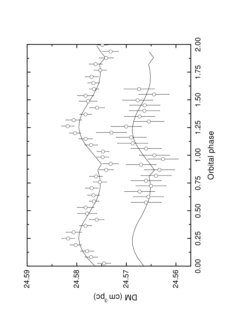
Figure 2: The measuredfrei and predicted DM as a function of orbital phase in 47 Tuc J . The measured upper plot represents the measurement made with 1999-2002 high-resolution data, displayed $0.01$cm^-3 pc below their measured values for clarity. The second plot represent the DM obtained using only the data from the best observation (1999 October 11), displayed $0.02$cm^-3 pc below their measured valuesfrei . The solid curve of the upper plot represent the best fit. And the solid curve of the second plot is obtained by setting the time 0.3714 year later than the upper fitting.

DM variation with the orbital phase is clearly detected in 47 Tuc J, as shown by the scattered points with error bars in Fig 2. The variation has been interpreted as a cometary-like phenomenon, which caused by material at a considerable distance from the companion, with much higher average electron density than that of the rest area. In other words, the plasma cloud is responsible for the additional time delay, which can be attributed to the variations of DM .

Whereas the variation of DM and the residuals of TOAs as function of orbital phase are very close at different frequencies, from 660MHz to 1486MHzfrei . Which means that the additional time delay is not likely caused by the propagation effect of ISM. Since the time delay due to DM variations should be very different at low and high-frequency.

Actually, what measured in 47 Tuc J of Fig 2 is residual of TOAs, or additional time delay, $\Delta^{obs}$, which can be attributed to the variation of DM. And the discussion above indicates that such explanation is difficult to explain the frequency problem.

Therefore, we can transform the DM variation of Fig 2 back into the additional time delay, $\Delta^{obs}$, and try to interpret it by the dynamic effect.

The time delay, $\Delta^{obs}$, measured in the time interval between two moment, $t$ and $t+\tau$ (or orbital phases $\phi(t)$ and $\phi(t+\tau)$), corresponds to the DM variation, $DM(t)$ and $DM(t+\tau)$ respectively. The relationship between DM and $\Delta^{obs}$ can be given bymt77

$$\delta\Delta^{obs}=\frac{DM(t+\tau)}{2.41\times 10^{-4}f^{2}}-\frac{DM(t)}{2.41\times 10^{-4}f^{2}}\,.$$ (20)

Thus the geodetic precession induced time delay at two moment $t$ and $t+\tau$ given by Eq(17), can be used to explain the observational one represented by Eq(20), $\delta\Delta^{obs}$. The new interpretation can not only solve the difficulties in the previous explanations of 47 Tuc J, but also fit the additional time delay numerically.

The estimation above indicates that $\delta\Delta_{R}$, $\dot{x}$ and $\dot{P}_{b}$ can be well explained by the geodetic precession of the binary system. Now we can fit these variations numerically.

The vectors ${\bf S}_{1}$, ${\bf S}_{2}$ and ${\bf S}$ are studied in the coordinate system of the total angular momentum, in which the z-axis directs to ${\bf J}$, and the x- and y-axes are in the invariance plane. ${\bf S}$ can be represented by $S_{P}$ and $S_{V}$, the components parallel and vertical to the z-axis, respectively:

$$S=(S_{V}+S_{P})^{1/2}\ .$$ (21)

$S_{P}$ and $S_{V}$ can be expressed (recall $S_{V1}$, $S_{V2}$ and $S_{V}$ form a triangle) as

$$S_{P}=S_{1}\cos\lambda_{JS1}+S_{2}\cos\lambda_{JS2}\ ,$$

$$S_{V}=(S_{V1}^{2}+S_{V2}^{2}-2S_{V1}S_{V2}\cos\eta_{S1S2})^{1/2}\ ,$$ (22)

where $\eta_{S1S2}$ is the misalignment angle between $S_{V1}$ and $S_{V2}$, which can be written as

$$\eta_{S1S2}=(\Omega_{1}-\Omega_{2})t+\phi_{i}\ .$$ (23)

Therefore, by the variation of $S$ as function of time (in the case of one spin, $S=$const), we can obtain $\Omega_{0}$ as function of time through Eq(4). Thus the measured $\Delta^{obs}$ of Eq(20) (or $\dot{DM}$) can be fitted step by step through Eq(17).

$$\delta\Delta^{obs}=\delta\Delta_{R}^{t+\tau}-\delta\Delta_{R}^{t}\ .$$ (24)

Through Eq(9) and Eq(7), the measured secular variabilities, $\dot{P}_{b}^{obs}$ and $\dot{x}^{obs}$frei , can also be fitted along with $\Delta^{obs}$ by Monte-Carlo method. Obviously the long-term and short-term together imposes very stringent constraints on the numerical solutions. Notice that the measured mass function, $f_{1}(M_{\odot})=4.864\times 10^{-6}$frei is also considered in the fitting.

As shown in Eq(9) and Eq(7), $\Omega_{0}$ is included in $\delta\Delta_{R}$ and $\dot{x}$, meanwhile $\dot{\Omega}_{0}$ is included in $\dot{P}_{b}$. Both $\Omega_{0}$ and $\dot{\Omega}_{0}$ contain $S(t)$, $S_{1}$ and angles, as shown in Eq(4) and Eq(8). Therefore, fitting the short-term and long-term parameters lead to the determination of $S_{1}$ and $S_{2}$, and in turn the moment of inertia of the pulsar, $I_{1}$, since the pulsar period is known.

In numerical fitting, $S_{1}$ and $S_{2}$ are fitted in the range $[2.5\times 10^{46},1.4\times 10^{49}]$ and $[2.5\times 10^{46},7.6\times 10^{49}]$ (g cm²s^-1) respectively, which are enough to cover the estimated values. The best solution is shown in Table I. By Eq(20) and Eq(4), we have $\dot{DM}\propto\delta\Delta_{R}\propto\Omega_{0}\propto S_{1}$, thus the $30\%$ errors in the DM variation in the upper plot of Fig 2, can cause about $30\%$ error in the fitted results, such as $S_{1}$ and $I_{1}$.

After fitting the measured time delay by the predicted one, as Eq(24), we can transform the predicted one, at the right hand side of Eq(24) into the theoretical DM variation, as displayed by the solid curves of Fig 2. So that it can be compared with the measured ones more clearly.

The measured DM variation are slightly different at different time, i.e., 1998 June and 1999 October, as shown in Fig 2 (points with error bars), which can be explained by Eq(16) from which $\delta\Delta_{R}$ are slightly different at different time.

V PSR J0621$+$1002

For PSR J0621$+$1002, dramatic variability of its DM has been measured, with gradient as steep as 0.013 pc cm^-3yr^-1, shown in Fig 3. By the standard picture, the turbulence spreads energy from longer to shorter length scales arises a power law of the structure function, which is given by $D_{DM}(\tau)\equiv\langle[DM(t+\tau)-DM(t)]^{2}\rangle$, where $\tau$ is the time lag between DM measurement. However the structure function obtained from observation obviously deviates from the simple power lawspl . Moreover, there is also no obvious differences in DM variation corresponding to 430 and 1410 MHzspl . Which indicates that DM variation of this binary pulsar is also independent of frequency. In the geodetic precession induced model these difficulties can be explained naturally.

Similarly, with $m_{1}=1.70M_{\odot}$, $m_{2}=0.97M_{\odot}$, $e=0.00246$, ${P}_{b}=8.3$d and $x=12$frei , we have $\Omega_{1}=1.4\times 10^{-12}$s^-1, $\Omega_{2}=2.2\times 10^{-12}$s^-1. Assuming $\Omega_{0}\approx\Omega_{2}$, the geodetic precession induced time delay given by Eq(18) can be written as ($\tau=1$yr)

$$|\delta\Delta_{R}|\approx x\Omega_{0}\tau|\cos(\omega)|\approx 8.3\times 10^{-4}(s)\,,$$ (25)

The measured maximum DM variation, $\dot{DM}=0.013$pc cm^-3yr^-1spl , corresponds to a delay of $\Delta^{obs}=2.9\times 10^{-4}$s per year. Therefore the predicted one and the measured one can be consistent.

VI 47 Tuc H

The DM variation of 47 Tuc H, $\dot{DM}=-0.024(3)$cm^-3pc yr^-1 (equivalent $\Delta_{R}=5.4\times 10^{-4}$s per year), is one of the largest DM variations for any pulsar, and no binary parameters available can explain the trendfrei . Whereas the geodetic precession model can explain this large DM variation easily.

By the same treatment as the two binaries above, with $m_{1}=1.50M_{\odot}$, $m_{2}=0.186M_{\odot}$ and $x^{obs}=2.15$frei , the additional time delay per year is approximately, $\Delta_{R}\approx 1.8\times 10^{-4}$s, in the case $\Omega_{0}\approx\Omega_{1}\approx 2.7\times 10^{-12}$s^-1; and $\Delta_{R}\approx 1.2\times 10^{-3}$s, in the case $\Omega_{0}\approx\Omega_{2}\approx 1.7\times 10^{-11}$s^-1. Therefore, the large $\dot{DM}$ measured in 47 Tuc H, which is $\Delta_{R}=5.4\times 10^{-4}$s per year, can be well explained by an orbital precession velocity that is in the range, $\Omega_{1}<\Omega_{0}<\Omega_{2}$.

VII discussion

As shown in Fig 4, the the orbital precession velocity, $\Omega_{0}$, can contribute to the orbital precession, absorbed by $\dot{x}$; apsidal motion, absorbed by $\dot{\omega}$; and nutation, absorbed by $\dot{P}_{b}$ respectively.

For very special NS–NS or NS–WD binary pulsars, $m_{1}=m_{2}$ or one spin is ignorable (i.e, $S_{1}=0$), ${\bf S}$ is a constant vector, then $\Omega_{0}$ is a constant, which means $\dot{\Omega}_{0}=0$, and in turn $\dot{P}_{b}=0$, therefore, there will be only static orbital precession and apsidal motion but no nutation. In such special cases the additional time delay can be absorbed by $\dot{x}$ and $\dot{\omega}$, of which $\dot{x}$ is a function of time (or orbital phase) and $\dot{\omega}$ is unchanged.

While for general NS–NS or NS–WD binary pulsars, $m_{1}\neq m_{2}$ and $S_{1}\neq 0$, $S_{2}\neq 0$, the two spins precesses at different velocities ($\Omega_{1}\neq\Omega_{2}$), therefore, ${\bf S}$ varies both in direction and magnitude (${\bf S}={\bf S}_{1}+{\bf S}_{2}$). Then $\Omega_{0}$ is a function of time by Eq(4) ($\dot{\Omega}_{0}\neq 0$), which leads to the nutation ($\dot{P}_{b}\neq 0$) by Eq(9). Therefore, for a general NS–NS or NS–WD binary pulsar, there is nutation effect beside the precession of the orbit and the apsidal motion.

Thus, for a general binary pulsar, the three constant parameters $\dot{x}^{obs}$, $\dot{\omega}^{obs}$, and $\dot{P}_{b}^{obs}$ together, can largely eliminate the trend of residuals, or the additional time delay which can be represented as $DM$ vs time, or $DM$ vs orbital phase.

Since $\Omega_{0}$ varies with time, then $\dot{x}$, $\dot{\omega}$ and $\dot{P}_{b}$ also vary with time, as shown by Eq(7), Eq(5) and Eq(9) respectively, whereas, the measured $\dot{x}^{obs}$, $\dot{\omega}^{obs}$ and $\dot{P}_{b}^{obs}$, are all constants, or the average values of the true effects, thus for such binary pulsar which have small orbital periods, i.e., a few hours ($\dot{x}^{obs}$ and $\dot{P}_{b}^{obs}$ vary rapidly), higher order derivatives, such as $\ddot{x}^{obs}$ and $\ddot{P}_{b}^{obs}$ are necessary to eliminate the trend of residuals. The fitting of the $DM$ vs orbital phase in 47 Tuc J in this paper actually included such higher order of derivatives, because $\dot{x}$, $\dot{\omega}$, and $\dot{P}_{b}$ used in fitting are given by Eq(7), Eq(5) and Eq(9) respectively, which are all functions of time.

The relationship of the geodetic precession induced secular variabilities and the additional Roemer time delay as well as the DM variation is summarized in Fig 3.

Therefore, comparing with the secular variations, $\dot{x}$ and $\dot{P}_{b}$, the variation of DM of 47 Tuc J is just the short-term effect ($t\approx P_{b}/20$) of geodetic precession in a binary pulsar.

$\dot{DM}$, and secular variabilities, such as $\dot{x}$ and $\dot{P}_{b}$, have been interpreted separately by different models. While the geodetic precession provides an unified model which can well explain these variabilities (both short term and long-term).

On the other hand, the DM variations provide new evidences of the geodetic precession effect in binary pulsar systems, beside the secular variabilities, and the theoretical prediction of the moment of inertia of neutron stars.

The numerical results of spin angular moment of white dwarf star and the pulsar, as well as moment of inertia of the pulsar provides very useful information on both the structure of white dwarf stars and neutron stars.

The interpretation of the DM variation by the dynamic effects in the three binary pulsars (the frequency problems in the previous explanation are solved automatically) indicts that the structure of the ISM between the these pulsars and the Earth might be very stable, which is similar as PSR B1855+09lob . This might provide new information in the understanding of ISM.

Table 1: Parameters obtained by fitting DM vs time, ${\dot{x}}^{obs}$ and ${\dot{P}_{b}}^{obs}$ of 47 Tuc J

$\lambda_{JS_{1}}$	$\lambda_{JS_{2}}$	$\lambda_{LS_{1}}$	$\phi_{i}$	$\omega_{i}$	$\eta_{i}$
$0.9192$	$1.476$	$0.9203$	$0.1095$	$3.594$	$0.3640$
$S_{1}$(g cm2s-1)	$S_{2}$(g cm2s-1)	$m_{1}$	$m_{2}$	$e$	$i$
$5.985\times 10^{48}$	$4.933\times 10^{49}$	$1.949$	$0.0264$	$1.929\times 10^{-5}$	$1.570$

By $S_{1}$ the moment of inertia of the pulsar can be obtained, $I_{1}=2.0\times 10^{45}$g cm². Notice that $m_{1}$ and $m_{2}$ are in sun mass, all angles are in radian. The errors of the values in the above table is about $30\%$

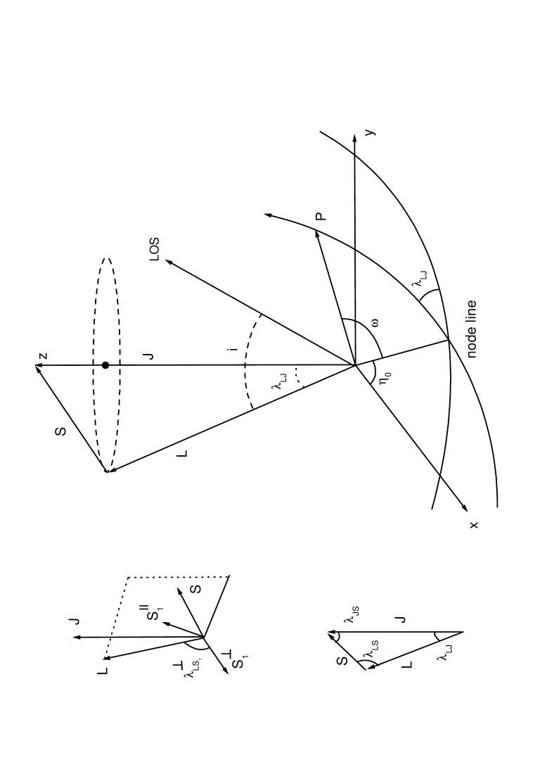
Figure 1: Binary geometry and definitions of angles. The invariable plane (x-y) is perpendicular to the total angular momentum, ${\bf J}$. The inclination of the orbital plane with respect to the invariable plane is $\lambda_{LJ}$, which is also the precession cone angle of ${\bf L}$ around ${\bf J}$. The orbital inclination with respect to the line of sight is $i$. $\eta_{0}$ is the phase of the orbital plane precession. $\omega$ is longitude of periastron (point P).

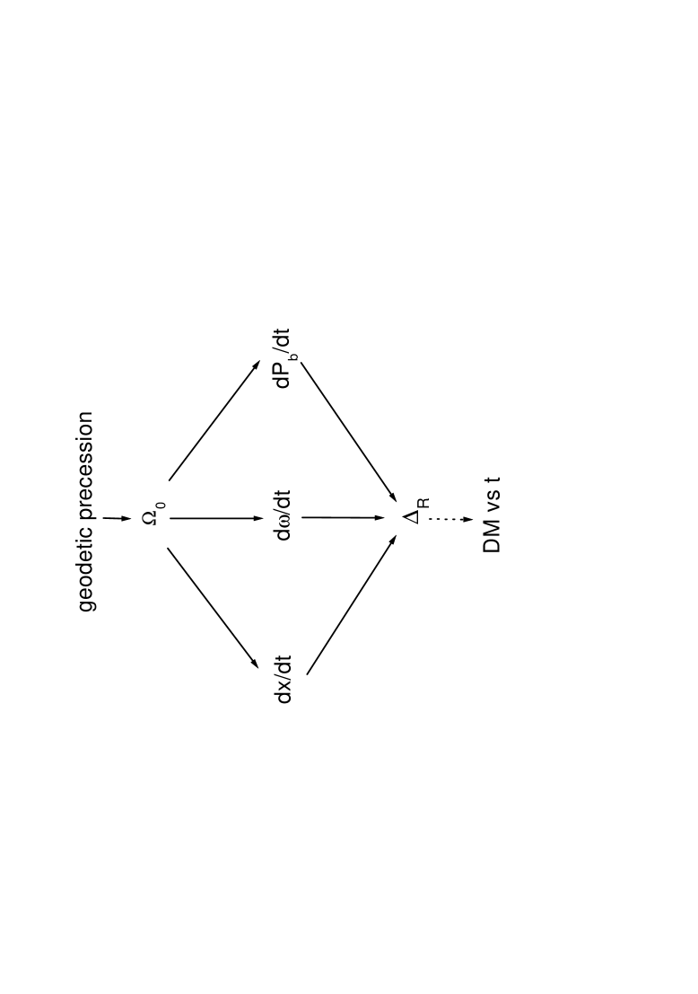
Figure 3: Geodetic precession leads to an additional orbital precession velocity, $\Omega_{0}$, which can be absorbed by three parameters, $\dot{x}$, $\dot{\omega}$ and $\dot{P}_{b}$. Which in turn cause an additional time delay, $\Delta_{R}$, which can be attributed to DM variation.

References

- (1) R.N. Manchester and J.H. Taylor, W.H. Freeman and Company San Francisco (1977).
- (2) P.C. Freire, and F. Camilo et al, MNRAS, 340, 1359-1374 (2003).
- (3) E.M.Splaver, and D.J. Nice, et al, Astrophys.J. 581, 509-518 (2002).
- (4) B.J. Rickett, ARAA, 28, 561-605 (1990).
- (5) B.P. Gong, submitted.
- (6) A. Lommen and D.C. Backer , 199th AAS Meeting.
- (7) B.M. Barker, and R.F. O’Connell, Phys. Rev. D, 12, 329-335 (1975).
- (8) T.A. Apostolatos, C. Cutler, J.J. Sussman, and K.S. Thorne, Phys. Rev. D, 49,6274-6297 (1994).
- (9) L.E. Kidder, Phys. Rev. D, 52, 821-847 (1995).
- (10) L.L. Smarr, and R.D. Blandford, Astrophys.J. 207, 574-588 (1976).
- (11) S.M. Kopeikin, Astrophys. J 467, L93-L95 (1996).
- (12) J.H. Taylor and J.M. Weisberg, Astrophys. J 345, 434-450 (1989).