Abstract

High redshift quasars mark the locations where massive galaxies are rapidly being assembled and forming stars. There is growing evidence that quasar environments are metal-rich out to redshifts of at least five. The gas-phase metallicities are typically solar to several times solar, based on independent analyses of quasar broad emission lines and intrinsic narrow absorption lines. These results suggest that massive galaxies (e.g., galactic nuclei) experience substantial star formation before the central quasar becomes observable. The extent and epoch of this star formation (nominally at redshifts $z>2$, but sometimes at $z>5$) are consistent with observations of old metal-rich stars in present-day galactic nuclei/spheroids, and with standard models of galactic chemical evolution. There is further tantalizing (but very tentative) evidence, based on FeII/MgII broad emission line ratios, that the star formation usually begins $\geq$0.3 Gyr before the onset of visible quasar activity. For the highest redshift quasars, at $z\approx 4.5$ to $\sim$6, this result suggests that the first major star formation began at redshifts $\geq$6 to $\geq$10, respectively.

Chapter 0 Quasar Elemental Abundances
and Host Galaxy Evolution

1 Introduction

Quasars are no longer perceived merely as exotic high-redshift monsters. Rather, they are commonplace, in the sense that every massive galaxy today was at one time an active quasar host. Quasars are thus valuable probes of galaxy evolution. They light up the surrounding gas (in young galactic nuclei), and they provide a bright emission source for absorption line studies, during a poorly understood, early phase of galaxy assembly. This review describes measurements of the gas-phase elemental abundances near quasars, and the implications for massive galaxy evolution. Please see Hamann & Ferland (1999, hereafter HF99) for a more comprehensive review of this topic.

1 Quasars, Galaxies, & High-Redshift Star Formation

Recent studies show that quasars, or more generally Active Galactic Nuclei (AGNs), are natural byproducts of galaxy formation. The super-massive black holes (SMBHs) that power AGNs are not only common in the centers of galaxies, but the SMBH masses correlate directly with the mass of the surrounding galactic spheroid (Merrit & Ferrarese 2001, Gebhart et al. 2000, Tremaine et al. 2002). Whatever processes lead to the formation of galactic spheroids, e.g., elliptical galaxies and the bulges of grand spirals, must also (somehow) create a central SMBH with commensurate mass. Most of the SMBHs in galaxies today are “dormant," or nearly so, because the mass accretion has declined or ceased. But all of the galaxies hosting SMBHs today must have been at one time “active,” with the bright AGN phase corresponding to the final growth phase of the SMBH.

The bright AGN phase is expected to be brief. In the standard paradigm of AGN energy production, the mass accretion rate, $\dot{M}$, needed to maintain a given luminosity, $L$, is $L=\eta\dot{M}c^{2}$, where $\eta$ is an efficiency factor believed to be of order 0.1. The luminosity can also be expressed as a fraction of the Eddington limit, $L=\gamma\,L_{E}\approx(1.5\times 10^{46})\,\gamma M_{8}$ ergs s^-1, where $L_{E}$ is the Eddington luminosity, $M_{8}$ is the SMBH mass relative to $10^{8}$ M_⊙, and $\gamma$ is a constant typically between 0.1 and 1 for luminous quasars (Vestergaard 2003, Warner et al. 2003). If the bright AGN phase corresponds to the final accretion stage where the SMBH roughly doubles its mass while accreting at $\sim$50% of the Eddington rate ($\gamma\approx 0.5$), then the lifetime of this phase should be $\sim$$6\times 10^{7}$ yr (based on the expressions above). This nominal lifetime fits well with the population demographics. In particular, the observed space density of present-day SMBHs, with masses from $<$$10^{6}$ M_⊙ to $\sim$10¹⁰ M_⊙, can account for the high-redshift quasar population if every one of these SMBHs shined previously as an AGN for a few $\times 10^{7}$ yr (Ferrarese 2002).

Another important aspect of the AGN–galaxy relationship is the close link between AGNs and vigorous star formation. For example, high-redshift quasars are often strong sources of sub-mm dust emission, which is attributed to powerful starbursts in the surrounding galaxies (Omont et al. 2001, Cox et al. 2002). Several authors have noted that the growth in the quasar number density with increasing redshift matches well the increasing cosmic star formation rate (e.g., Franceschini et al. 1999). Quasars flourished at a time (corresponding to $z\sim 2$ to 3) when most massive galactic spheroids (e.g., elliptical galaxies and the bulges of grand spirals) were frantically forming most of their stars (Renzini 1998, Jimenez et al. 1999, Dunne et al. 2003). It seems likely that the same processes that dump matter into galactic nuclei to form an SMBH also induce substantial star formation.

All of this evidence indicates that high-redshift quasars are bright beacons marking the locations where massive galactic nuclei are being assembled — vigorously making stars and building a central SMBH. However, we may still have something like the old “chicken versus egg” problem. Which came first, the galaxy or the quasar? The bulk of the stars or the central SMBH? How mature are the host galaxies when the central AGN finally becomes visible?

2 Quasar Abundance Studies

Quasar abundance studies seek to examine quantitatively the chicken versus egg problem. How chemically enriched are quasar environments and, by inference, how much star formation preceded the observed quasars? Does the degree of enrichment depend on the type of AGN or on properties (mass?) of the surrounding host galaxy? When does the star formation begin in quasar environments? Are the host environments of high redshift quasars less evolved and therefore less metal rich? The answers to these questions will provide unique constraints on high-redshift star formation and early galaxy evolution.

Most of the effort in this field has been to measure the overall gas-phase metallicities near quasars. But there is still more we can learn from the relative metal abundances. The ratio of iron to $\alpha$ elements is of particular interest because the $\alpha$ elements, such as O, Ne, and Mg, derive exclusively from massive-star supernovae (Types II, Ib and Ic), while Fe has a dominant contribution from intermediate-mass stars via Type Ia supernovae (Yoshii et al. 1996). The SN Ia contribution of Fe is delayed relative to the SN II+Ib+Ic products because of the longer lifetimes of SN Ia precursors (integrated over a stellar initial mass function). The amount of the delay is often assumed to be $\sim$1 Gyr, but Matteucci & Recchi (2001) showed that this number depends on environmental factors such as the star formation rate and initial mass function. They argue that $\sim$0.3 Gyr is more appropriate for young elliptical galaxies/spheroids (with high star formation rates). In any case, the delay can be used as an approximate “clock” to constrain the formation times of stellar populations. For example, observations of large gas-phase Fe/$\alpha$ ratios near metal-rich quasars would indicate that their surrounding stellar populations are already $\geq$0.3 Gyr old.

1 Spectral Diagnostics

The first step is to understand the abundance diagnostics in quasar spectra. The signature features are the broad emission lines (BELs), with profile widths greater than 1000 – 1500 km s^-1. Reverberation mapping studies show that quasar BELs form in photoionized gas within $\sim$1 pc of the central continuum source (Kaspi et al. 2000). Some of the first quasar studies noted that BELs identify the same variety of elements (hydrogen, carbon, nitrogen, oxygen, etc.) seen in much less exotic stellar and galactic environments (Burbidge & Burbidge 1967). In particular, there are no obvious abundance “anomalies.” The first quantitative estimates of BEL region abundances (see Davidson & Netzer 1979 for an excellent review) confirmed the lack of abundance anomalies compared to solar element ratios, and showed further that the metallicities are probably within a factor of $\sim$10 of solar.

More recent abundance studies include absorption lines among the diagnostics. Quasar absorption lines are classified generically according to their full widths at half minimum (FWHMs). Roughly 10% to 15% of optically selected quasars have classic broad absorption lines (BALs), with FWHM $>$ 2000 to 3000 km s^-1. At the other extreme are the narrow absorption lines (NALs), which have typically FWHM $<$ a few hundred km s^-1. A useful working definition of the NALs is that the FWHM is not large enough to blend together important UV doublets, such as C IV $\lambda\lambda$1548,1551, whose velocity separation is 500 km s^-1. Intermediate between the NALs and BALs are the so-called mini-BALs. The BALs and mini-BALs appear exclusively blueshifted with respect to the emission lines, with velocity shifts from near 0 km s^-1 to $>$30,000 km s^-1 in some cases. Their broad and smooth profiles at blueshifted velocities clearly identify outflows from the central quasar energy source. NALs are also frequently blueshifted, but they can appear at redshifted velocities up to $\sim$2000 km s^-1. NALs within $\pm$5000 km s^-1 of the emission line redshift are also called “associated” absorption lines (AALs). In general, NALs can form in a wide range of environments, from high speed outflows like the BALs to cosmologically intervening clouds or galaxies having no relation to the quasar. One challenge in using NALs for abundance work is to understand the location of the absorbing gas.

The following sections outline the procedures and results related to each of these diagnostics. Please see HF99 for a more complete discussion.

3 Intrinsic Narrow Absorption Lines (NALs)

Figure 1 shows some typical examples of associated NALs in the spectrum of a bright quasar, PG 0935+417 with emission-line redshift $z_{em}=1.966$. The AALs in this case have FWHMs from $\sim$12 to $\sim$133 km s^-1, and they are blueshifted by $\sim$1400 km s^-1 to $\sim$3000 km s^-1 with respect to $z_{em}$.

Figure 1: Normalized Keck–HIRES spectra of “associated” NALs in the quasar PG 0935+417. Strong doublets are labelled above with open brackets: C IV $\lambda\lambda$1548,1551, N V $\lambda\lambda$1238,1242, and Si IV $\lambda\lambda$1393,1403. The velocity scale is relative to $z_{em}$ = 1.966 for the short wavelength component of each NAL doublet. The dotted vertical lines mark the velocities of the six strongest C IV systems.

There are three critical steps involved in using NALs as abundance diagnostics. First, we must distinguish the intrinsic NALs from those that form in unrelated, cosmologically intervening gas. We define “intrinsic" NALs loosely as forming in gas that is (or was) part of the overall AGN/host galaxy environment. Statistical studies suggest that the AALs are often intrinsic to the quasar/host galaxies (Richards et al. 1999, Foltz et al. 1986). Other observational criteria must be applied to determine which specific NALs are intrinsic, such as, i) time-variable line strengths, ii) NAL profiles that are broad and smooth compared to the thermal line width, iii) excited-state absorption lines that require high gas densities, and iv) NAL multiplet ratios that reveal partial line-of-sight coverage of the background light source (see Hamann et al. 1997a, Barlow & Sargent 1997). Characteristics like variability, broad-ish line profiles, and partial covering often appear together, clearly indicating an intrinsic origin. Some NALs show none of these characteristics and the location of their absorbing gas remains ambiguous.

Second, we must derive column densities in a way that can account for an absorber that might be inhomogeneous and/or partially covering the background light source(s). In the most general case, the observed line “intensities” represent an average of the intensities transmitted over the projected area of an extended emission source(s). If the absorber happens to be homogeneous (has a constant line optical depth) across the face of a uniformly bright emission source, then the observed intensity is simply,

$${{I(\lambda)}\over{I_{o}(\lambda)}}\ =\ 1\,-\,C_{f}(\lambda)\,+\,C_{f}(\lambda)\,e^{-\tau_{\lambda}}$$ (1)

where $I_{o}(\lambda)$ is the intensity of the emission source at wavelength $\lambda$, $\tau_{\lambda}$ is the line optical depth, $C_{f}(\lambda)$ is the coverage fraction of the absorbing material ($0\leq C_{f}(\lambda)\leq 1$), and we ignore small contributions of line emission from the absorbing gas. If we measure two absorption lines having a known optical depth ratio, e.g., in a doublet, then we can use the measured strengths and ratios of those lines (providing two equations) to solve uniquely for both $\tau_{\lambda}$ and $C_{f}(\lambda)$ at each wavelength (Petitjean et al. 1994, Hamann et al. 1997, Barlow & Sargent 1997). For resonance lines, the ionic column densities then follow simply from the optical depths, $N_{ion}\propto\ \int\tau_{\lambda}\,d\lambda$. The key is to obtain high-resolution spectra (so there are no unresolved line components) of NAL multiplets. Fortunately, there are many possibilities, such as the doublets shown in Figure 1.1, the H I Lyman series lines, and others.

If the absorbing medium is inhomogeneous, then more lines are needed to define the two-dimensional optical depth/column density distribution. However, a simple doublet analysis still provides a useful estimate of the optical depth spatial distribution (at each wavelength), subject to an assumed functional form for that distribution. We recently completed an extensive theoretical study of the effects of inhomogeneous absorption on observed absorption lines (Sabra & Hamann 2003), which builds upon the pioneering work of deKool et al. (2001). We find that, for a wide range of inhomogeneous optical depth distributions, the spatially averaged value of the optical depth is very similar to the single value one would derive (from the same data) assuming homogeneous partial coverage (Eqn. 1.1). Therefore, the most general situation effectively reduces to the simple homogeneous case for the purposes of an abundance analysis.

The final step is to convert ratios of ionic column densities into abundance ratios using ionization corrections. The correction factors can be large because NALs are often highly ionized and we must compare a high ion, such as C IV, to H I Ly$\alpha$ to estimate the C/H abundance (metallicity). There can also be a range of ionizations present in the absorber but not enough measured lines to fully characterize this range. Nonetheless, Hamann (1997) showed that we can always derive conservatively low estimates of the metal/hydrogen abundance ratios by assuming each metal line forms under conditions that most favor that ion. In particular, we can use the maximum possible value of the metal ion fractions, such as C IV/C, as indicated by photoionization calculations. Similarly, there are minimum ionization corrections for each metal ion that provide firm lower limits on the metal/hydrogen abundance (see also Bergeron & Stasinska 1986). These conservative estimates and firm lower limits provide useful constraints on the metallicity even if we we have no knowledge of the degree or range of ionizations in the gas (see also HF99).

1 Results

High resolution spectra suitable for NAL abundance studies did not become available until the 1990s. The earliest results (Wampler et al. 1993, Petitjean et al. 1994, among others) were confirmed by later studies (Hamann 1997, Hamann et al. 1997a, Tripp et al. 1996, Savage et al. 1998, Petitjean & Srianand 1999, Papovich et al. 2000). Quasar AALs often have metallicities $Z\geq$ Z_⊙. Several of these studies also report N/C above solar, although in most cases the data are not adequate for this measurement. So far there are only two published reports (to our knowledge) of AAL abundances above redshift 4, and the results are slightly mixed. Wampler et al. (1996) estimated $Z\sim 2$ Z_⊙ based on the tentative detection of O I $\lambda$1303 in one AAL system at redshift 4.67, while Savaglio et al. (1997) reported $0.1\leq Z\leq 1$ Z_⊙ for an AAL complex at redshift 4.1. However, in both of these cases, and many others, the location of the absorber is not known. All of the confirmed intrinsic NALs (based on the criteria mentioned §1.3) have metallicities $Z\geq$ Z_⊙ (see refs. above). Petitjean et al. (1994) used a small sample of redshift $\sim$2 quasars to show that there is a dramatic decline in absorber metallicity as one moves away from the quasar emission redshift, from $Z\geq$ Z_⊙ in the AALs to $Z<0.1$ Z_⊙ at velocity shifts $\geq$10,000 km s^-1 (see their Figure 14, also Carswell et al. 2002). This result meets our expectation that AALs are often intrinsic to quasars, while most NALs at lower redshifts are unrelated (Rauch 1998).

There is a strong need now to improve on some of the early measurements and expand the database. We and collaborators have obtained high-resolution (7–9 km s^-1) spectra of 15 AAL quasars at $z_{em}\approx 2$ – 3 using the HIRES echelle spectrograph on the 10 m Keck I telescope. As a brief example consider the AALs of quasar PG 0935+417 shown in Figure 1.1. We find no evidence of line variability (above $\sim$10%) based on several observations that span $\sim$2 years in the quasar rest frame. Nonetheless, the three systems of C IV doublets at 3000 to 2700 km s^-1 are clearly intrinsic because of the large non-thermal line widths and doublet ratios that imply partial line-of-sight coverage of the background light source (see also Hamann et al. 1997b). The location of the three narrower absorption systems at 1700 to 1400 km s^-1 remains unclear. However, a preliminary analysis of all of these lines (based on simple equivalent width measurements and assuming constant coverage fractions across the profiles) suggests that the metallicities in all cases are $\sim$1 to $\sim$3 Z_⊙. A more detailed analysis of this data set is underway, but solar or higher metallicities appear to be common in the AALs, in agreement with earlier studies.

4 Broad Absorption Lines & Mini-BALs

Figure 1.2 shows the rest-frame UV spectrum of a fairly typical BAL quasar, PG 1254+047. The BALs in this case imply outflow velocities from roughly 15,000 to 27,000 km s^-1. The main obstacle to using BALs for abundance work is that the broad profiles blend together all the important doublets. Therefore, unlike the NALs, we cannot examine the doublet ratios for evidence of partial line-of-sight coverage. If we simply assume that the coverage fraction is unity ($C_{f}=1$ in Eqn. 1.1), then measurements of the column densities imply bizarre abundance ratios, such as, [Si/C] $>$ 0.5 and [C/H] $\approx 1$ to 2 (where [$x/y$] = $\log(x/y)-\log(x/y)_{\odot}$). The surprising detections of P V $\lambda\lambda$1118,1128 BALs in at least half of the well-measured sources, including PG 1254+047 (Fig. 1.2), imply [P/C] $\geq$ 1.6 (Junkkarinen et al. in prep., Hamann 1998, Hamann et al. 2002a, and refs. therein).

Figure 2: Hubble Space Telescope spectrum of PG 1254+047 ($z_{em}=1.01$) showing its strong BAL troughs. The BALs are labelled just above the spectrum, while the prominent broad emission lines are marked across the top. The measured flux has units 10^-15 ergs/s/cm²/Å. From Hamann (1998).

The most likely explanation for these strange abundances is that they are incorrect. BALs are often much more optically thick than they appear because the absorber partially covers the background light source(s). Direct evidence for partial coverage has come from comparisons of widely spaced line pairs (similar to the doublet analysis but not involving doublets) in one well-measured BAL quasar (Arav et al. 2001). Doublet ratios in borderline NALs/mini-BALs, sometimes embedded within BAL profiles and believed to form in the same general outflow, also frequently indicate partial coverage (Hamann et al. 1997b, Barlow, Hamann & Sargent 1997, Telfer et al. 1998, Srianand & Petitjean 2000). Less direct evidence comes from spectropolarimetry of scattered light in BAL troughs (Schmidt & Hines 1999), and from flat-bottomed BAL profiles that “look” optically thick even though they do not reach zero intensity.

Another clue comes from the surprisingly strong P v BALs. Hamann (1998) noted that the P V line should be nominally weak. Its ionization is very similar to C IV, but in the Sun phosphorus is $\sim$1000 times less abundant than carbon. Therefore, if the P/C abundance is even close to solar in BAL regions, the P V line should not be present unless C IV and the other strong BALs of abundant elements are much more optically thick than they appear. In other words, there is partial coverage and unabsorbed light fills in the bottoms of BAL troughs. If we turn that argument around and assume solar P/C in PG 1254+047 (Fig. 1.2), we find that the true optical depth in its C IV line is $\geq$25 (Hamann 1998).

This interpretation of the P V may be disputed by Arav et al. (2001), who measured P V and many other BALs in one quasar spectrum with extraordinarily wide wavelength coverage. They estimate a metallicity near solar but [P/C] $\geq$ 1. If that P/C result is correct, it would probably require a unique enrichment history (e.g., involving novae, Shields 1996). However, the uncertainties and challenges are substantial. We prefer to exclude BALs from quasar abundance studies.

5 Broad Emission Lines

Figure 1.3 shows part of the rest-frame UV spectrum of a quasar at redshift $z_{em}=4.16$. The emission lines shown in this plot, plus C III] $\lambda$1909, have formed the basis for many BEL metallicity studies. The main advantage of the BELs is that they can be measured in any quasar using moderate resolution spectra. There is also no question that the lines form close to the quasar, nominally within $\sim$1 pc of the central engine (§1.2.1).

One issue affecting the BEL analysis is that the emitting regions span simultaneously a wide range of densities and ionizations, with the higher ionizations occurring preferentially nearer the central continuum source (e.g., Ferland et al. 1992, Peterson 1993). Consequently, different lines can form in spatially distinct regions. Without a detailed model of the BEL environment, it is important for abundance studies to compare lines that form as much as possible in the same gas with similar excitation and radiative transfer dependencies. However, the range of physical conditions present in BEL regions provides a simplification: observed BEL spectra are flux-weighted averages over a diverse ensemble of “clouds.” The tremendous advantage of this natural averaging is that we do not need to derive, or make specific assumptions about, the physical conditions in the different line emitting regions (Hamann et al. 2002). The formalism developed to simulate this situation (Baldwin et al. 1995) has been dubbed the Locally Optimally-emitting Cloud (LOC) model, because each line forms naturally where the conditions most favor its emission.

Figure 3: Broad emission lines in the rest frame UV spectrum of the redshift 4.16 quasar, BR 2248$-$1242. The lower panel is an expanded version of the upper plot. From Warner et al. (2002).

Another important consideration is that the combined emission in the metal lines is not sensitive to the overall metallicity. In particular, the strengths of prominent metal lines, such as C IV, relative to the hydrogen lines, such as Ly$\alpha$, are not sensitive to the metal-to-hydrogen abundance ratio (HF99). The main reason is that these BELs are the dominant coolants in the photoionized plasma where they form. Radiative equilibrium requires that the total energy emitted from any region in the plasma equals the total energy absorbed. Therefore, changing the metallicity by factors of several cannot produce a commensurate change in the overall line strengths without violating energy conservation.

Nonetheless, BELs are sensitive to the metal abundances in several ways (see Ferland et al. 1996, HF99, Hamann et al. 2002). First, departures from solar metallicity by orders of magnitude will change the total metal/H line emission ratio (as well as individual line ratios such as C IV/Ly$\alpha$). For example, at very low metallicities ($\leq$0.03 Z_⊙) the metal lines no longer control the cooling and their emission strengths decline roughly commensurate with the metal/H abundance. This fundamental sensitivity to the extremes implies that typical BEL metallicities are conservatively within a factor of $\sim$30 of solar. Second, weak metal lines that are not important for the cooling do vary significantly with metallicity (while still preserving the overall energy balance). Abundance studies should, therefore, endeavor to include weaker lines, such as O III] $\lambda$1663 and N III] $\lambda$1750 (Fig. 1.3). Finally, the relative strengths of different metal lines can be sensitive to the metal/metal abundance ratios.

Taking advantage of this last point, Shields (1976) noted that in galactic H II regions the N/O abundance scales roughly proportional to O/H (metallicity) because of a strong “secondary” contribution to the nitrogen enrichment (see also Pettini et al. 2002, Pilyugin et al. 2003). The N/O $\propto$ O/H scaling dominates for metallicities above a few tenths solar. The N/O abundance therefore provides an indirect indicator of the overall metallicity. This technique has become the norm for BEL metallicity studies.

It should be noted that departures from the simple N/O $\propto$ O/H scaling can occur if there are metallicity-dependent stellar yields, or if the enrichment is dominated by star formation in discrete bursts (Kobulnicky & Skillman 1996, Henry et al. 2000). The latter situation would lead to time-dependent fluctuations in N/O because of different delays in the stellar release of N and O. However, the overall trend for increasing N/O with O/H remains, and the best homogeneous data sets indicate that the scatter in the N/O $\propto$ O/H relation declines with increasing O/H (Pettini et al. 2002, Pilyugin et al. 2003). This is the regime of quasars. Moreover, there are no reports, to our knowledge, of high N/O ratios (solar or higher) in metal poor (significantly sub-solar) interstellar environments. Large N/O abundances are an indicator of high metallicities in any scenario that involves well-mixed interstellar gas. The situation with N/C can also be complicated because N and C arise from different stellar mass ranges, leading again to time-dependent effects (Henry et al. 2000, Chiappini et al. 2003). Nonetheless, for the BEL analysis, it is generally assumed that to first order N/C behaves like N/O.

1 Results: Metallicity

Shields (1976) analyzed several ratios of UV intercombination (semi-forbidden) lines (see Fig. 1.3) and found that N/O and N/C are nominally solar to $\sim$10 times solar, consistent with solar to super-solar metallicities (see also Baldwin & Netzer 1978, Davidson & Netzer 1979, Uomoto 1984). Hamann & Ferland (1993) and Ferland et al. (1996) later claimed that the metallicities are typically several times solar, based on a new analysis of the N V/C IV and N V/He II BEL ratios. More recently, Hamann et al. (2002b) used extensive photoionization calculations to quantify better the abundance sensitivities of all of these nitrogen line ratios. In particular, they explored the influence of non-abundance effects such as density, ionization, turbulence, and incident continuum shape, in the context of LOC calculations. They favored N III]/O III] and N V/(C IV + O VI $\lambda$1034) as the most robust indicators of the relative N abundance. N V/He II is also very useful, but it has a greater sensitivity to the ionizing continuum shape because it compares a collisionally-excited line (N V) to a recombination line (He II, see also Ferland et al. 1996). Holding other parameters constant, the nitrogen line ratios scale almost linearly with the N/O and N/C abundances and should, therefore, be proportional to the metallicity if the enrichment follows N/O $\propto$ O/H.

Dietrich & Hamann (2003a) used the Hamann et al. (2002b) calculations to estimate BEL metallicities in a sample of $\sim$700 quasars spanning redshifts $0\leq z_{em}\leq 5$. They find typically several times Z_⊙ across the entire redshift range. Figure 1.4 shows results for a sub-sample of these quasars at $z_{em}\geq 3.5$, where the average metallicity is $\sim$5 Z_⊙ (from Dietrich et al. 2003b). Notice that there is no evidence of a metallicity decrease at the highest redshifts. For the particular $z_{em}=4.16$ quasar shown in Figure 1.3, where many lines are measurable owing to the narrow profiles and large equivalent widths, Warner et al. (2002) estimated $Z\approx 2$ Z_⊙. Dietrich et al. (2003a and 2003b) noted that the metallicities derived from the N V lines ratios (most notably N V/He II) are typically $\sim$30% to a factor of $\sim$2 larger than estimates from the intercombination ratios (e.g., N III]/O III]). The reason for this discrepancy is not clear. It could arise from systematic measurement errors in the weaker lines (Warner et al. 2003), or, perhaps, from subtle excitation/radiative transfer effects in the emitting regions. In any case, a factor of $\leq$2 agreement among the different BEL diagnostics is quite good. Our current strategy is to average the results from the various nitrogen BEL ratios.

The absolute uncertainties are more difficult to quantify because they depend on the theoretical techniques and assumptions. Factors of a few can be expected, but the essential result seems secure. The metallicities in quasar BEL regions are minimally near solar and perhaps typically several times above solar. This result is confirmed in general terms by the AAL data (§1.3.1, see also Kuraszkiewicz & Green 2003).

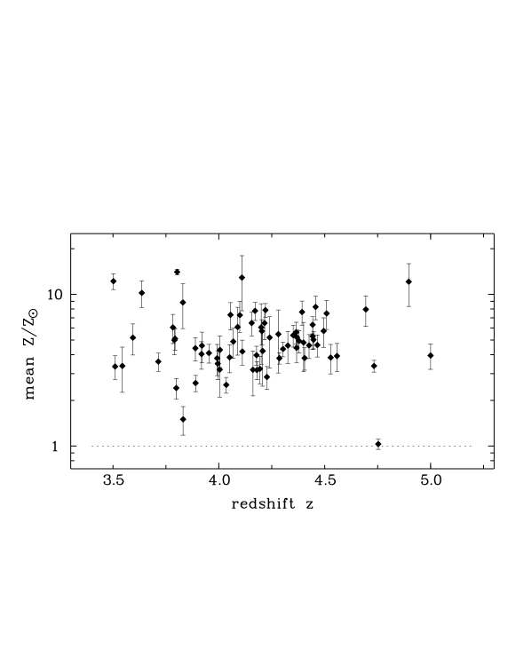
Figure 4: Average metallicities derived from BEL ratios in a sample of high redshift quasars. The error bars represent only the measurement uncertainties. From Dietrich et al. (2003b.)

Another interesting result from the BELs is that more luminous quasars appear to be more metal rich (Hamann & Ferland 1993, Osmer et al. 1994, HF99, Dietrich et al. 2003a). This trend is somewhat tentative because it is stronger in the N V/C IV and N V/He II ratios than in the intercombination lines, and it has not yet been tested in the AAL data. Nonetheless, it meets simple expectations. More luminous quasars are powered by more massive SMBHs, which reside in more massive galaxies (§1.1). There is a well-known relationship between mass and metallicity in normal galaxies (e.g., Trager et al. 2000), which is generally attributed to the effects of galactic winds. Massive galaxies reach higher metallicities because they retain their gas longer against the building thermal pressures from stellar mass loss and supernova explosions. Therefore, the gas near quasars in more massive galaxies could be more metal rich. Warner et al. (2003) tried to test this idea by comparing BEL metallicities to estimates of the SMBH masses (which serve as a surrogate for the host galaxy mass) in the large quasar sample of Dietrich et al. (2003a). The results are uncertain, but they do favor a trend between SMBH mass and BEL metallicity, as expected. In fact, our best estimate for the slope of this trend agrees well with the mass–metallicity slopes observed in galaxies.

2 Results: Fe/$\alpha$

BELs are the only diagnostics used so far to estimate Fe/$\alpha$ abundances as an age discriminator(§1.2). This work has relied on Fe II(UV)/Mg II $\lambda$2798, where “Fe II(UV)” represents a broad blend of many Fe II lines between roughly 2000 and 3000 Å. This blend is by far the most prominent Fe II feature in quasar spectra, and its UV wavelength makes it measurable at the highest redshifts in the near infrared. The nearby Mg II doublet serves the $\alpha$-element representative with an ionization similar to Fe II.

Measuring the flux in the broad Fe II blend presents a unique challenge (see Dietrich et al. 2003c for discussion). Spectra with wide wavelength coverage are essential to properly define the underlying continuum. It also helps to use a scaled template to fit the Fe II blend, based on either theoretical predictions (Wills et al. 1985, Verner et al. 1999, Sigut & Pradhan 2003) or observations of a well-measured source (Vestergaard & Wilkes 2001).

The main difficulty, however, is understanding the theoretical relationship between the Fe II/Mg II emission ratio and the Fe/Mg abundance. The Fe II atom has hundreds of relevant energy levels and thousands of lines that can blend together and/or contribute to radiative pumping/fluorescence processes. Current interpretations of observed Fe II spectra are still based largely on the pioneering calculations by Wills et al. (1985). Their work suggests that the strong Fe II fluxes from typical quasars require a relative iron abundance (e.g., Fe/Mg) that is super-solar by a factor of roughly 3. More modern calculations (Verner et al. 1999 and this proceedings, Sigut & Pradhan 2003, Baldwin et al. in prep.) use better atomic data and can, for the first time, incorporate a many-level Fe II atom into fully self-consistent treatments of the energy budget. So far these calculations have mostly just confirmed what Wills et al. knew already, that the uncertainties are large. However, work is now underway to understand these uncertainties. In particular, it will be important to quantify the sensitivities of the Fe II emission and the Fe II/Mg II ratio to various poorly-constrained, non-abundance parameters in BEL regions. It might turn out that the Fe II(UV)/Mg II ratio is not the best Fe/$\alpha$ diagnostic (Verner et al. this proceedings).

Putting these concerns aside for the moment, the observational results are becoming increasingly interesting. The best data indicate that the Fe II/Mg II emission ratio is the same on average at all redshifts (Thompson et al. 1999, Iwamuro et al. 2002, Dietrich et al. 2002 and 2003c and this proceedings). This includes the most recent observations of two quasars at redshifts $z_{em}\approx 6$ (Freudling et al. 2003). If we accept the tentative Wills et al. (1985) result that Fe/Mg is nominally above solar in BELs, which they deduced from spectra of quasars with $z_{em}\leq 0.5$, then the newer data suggest that Fe/Mg is large at all redshifts. Therefore, SN Ia’s played a role in the enrichment and the star formation must have begun at least 0.3 Gyr prior to the observed quasar epochs. For the redshift $\sim$6 quasars, this line of argument implies that the first major star formation occurred at redshift 10 – 20 (Freudling et al. 2003), consistent with the epoch of re-ionization deduced from recent WMAP data (Bennett et al. 2003).

6 Summary & Implications

Independent analysis of the BELs and intrinsic NALs indicates that quasar environments are metal rich at all redshifts. Typical metallicities range from roughly solar to several times solar. There might also be a trend with luminosity in the sense that more luminous quasars, which reside in more massive host galaxies, are more metal rich. If the gas near quasars was enriched by a surrounding stellar population, then the high metallicities indicate that those populations are already largely in place by the time the quasars “turned on” or became observable. For example, simple “closed-box” chemical evolution with a normal stellar initial mass function will produce metallicities above solar only after $\geq$60% of the original mass in gas is converted to stars. The quasar data imply that this degree of enrichment and evolution is common in massive galactic nuclei before redshift 2, and sometimes it occurs before redshift 5.

Unfortunately, the quasar data do not tell us the size (mass) of the stellar population responsible for the enrichment. However, the mass of gas in the BEL region sets a lower limit. The most recent estimates indicate that luminous quasars have BEL region masses that are conservatively $\sim$10³ to 10⁴ M_⊙ (Baldwin et al. 2003). Normal galactic chemical evolution then suggests that the stellar population needed to enrich this gas to $Z\geq$ Z_⊙ is ten times more massive, or $\sim$10⁴ to 10⁵ M_⊙. This mass may still be just the “tip of the iceberg” if one considers that quasar BEL regions are part of a much more massive reservoir that includes a $\geq$$10^{9}$ M_⊙ SMBH and its surrounding accretion disk. BEL regions might, in fact, be constantly replenished by the flow of material through the accretion disk. If that flow is $\sim$10 M_⊙ yr^-1 of metal-rich gas (§1.1), then clearly a much more massive stellar population (perhaps with Galactic bulge-like proportions) would be needed for the enrichment (see Friaça & Terlevich 1998 for specific enrichment models). for Observations of strong dust and sometimes CO emissions from high-redshift quasars (currently up to $z_{em}\approx 4.7$) indicate that there is often already $\geq$$10^{10}$ M_⊙ of metal-enriched gas present (Omont et al. 2001, Cox et al. 2002). There must have been massive amounts of star formation in these quasar host galaxies before the observed quasar epoch. Efforts to date the stellar populations around quasars using Fe II/Mg II BEL ratios suggest that the star formation often begins in earnest $\geq$0.3 Gyr prior to the appearance of a visible quasar. These results are tentative because of theoretical uncertainties, but for the highest redshift quasars yet studied ($z_{em}\approx 6$) they suggest that the first star formation occurred at $z\sim 10$ – 20.

In terms of the “chicken versus egg" problem (§1.1) the quasar abundance data are clear; a substantial stellar population is already in place by the time most quasars become visible. At low redshifts, direct imaging studies of quasars and their lower-luminosity cousins, the Seyfert 1 galaxies, show clearly that the host galaxies are already present with substantial, even moderately old, stellar populations on $>$ kpc scales (Nolan et al. 2001, Dunlop et al. 2003). At higher redshifts there is less direct imaging data, but at least some quasars still have substantial hosts (Kukula et al. 2001). It could be that the stars and the SMBH begin forming at the same time. But visible quasar activity might be delayed with respect to the surrounding star formation, even at the highest redshifts, because of the time needed to assemble the SMBH and/or blow out the dusty interstellar medium that obscures the youngest AGNs from our view (see also Romano et al. 2002, Kawakatu & Umemura 2003). This delay could explain observations showing that the quasar number density declines dramatically with increasing redshifts above $z\sim 3$, while the cosmic star formation rate appears to stay roughly constant out to at least $z\sim 4$ (Ivison et al. 2002).

Acknowledgements.  We are grateful to our collaborators, especially Jack Baldwin, Tom Barlow, Gary Ferland, Vesa Junkkarinen, and Kirk Korista, who contributed insights and unpublished results to this review. We also acknowledge NSF grant AST99-84040.

References

- [1] Arav, N., et al. 2001, ApJ, 561, 118
- [2] Baldwin, J.A., Ferland, G.J., Korista, K.T., Hamann, F., Dietrich, M. 2003, ApJ, 582, 590
- [3] Baldwin J., Ferland G., Korista K.T., & Verner D. 1995, ApJ, 455, L119
- [4] Barlow T.A., Hamann F., & Sargent W.L.W. 1997, ASP Conference Series, 128, 13
- [5] Barlow T.A., & Sargent W.L.W. 1997, AJ, 113, 136
- [6] Bennett, C.L., et al. 2003, ApJ, in press (astro-ph/0302207)
- [7] Bergeron J., & Stasinska G. 1986, A&A, 169, 1
- [8] Burbidge, G., & Burbidge, E.M. 1967, in Quasi-Stellar Objects, New York: Freeman
- [9] Carswell, R., Schaye, J., & Kim, T.-S. 2002, ApJ, 578, 43
- [10] Chiappini, C., Romano, D., & Matteucci, F. 2003, MNRAS, 339, 63
- [11] Cox, P., et al. 2002, ApJ, 387, 406
- [12] Davidson, K., & Netzer H. 1979, Rev. Mod. Physics, 51, 715
- [13] de Kool, M., et al. 2001, ApJ, 548, 609
- [14] Dietrich M., Hamann, F., Appenzeller, I., Vestergaard, M. 2003c, ApJ, submitted
- [15] Dietrich, et al. 2003b, ApJ, 589, 722
- [16] Dietrich M., Appenzeller I., Vestergaard M., & Wagner S.J. 2002a, ApJ, 564, 581
- [17] Dietrich, M., & Hamann, F. 2003a, in prep.
- [18] Dunlop, J.S., McLure, R.J., Kukula, M.J., Baum, S.A., o’Dea, C.P., & Hughes, D.H. 2003, MNRAS, 340, 1095
- [19] Dunne, L., Eales, S.A., Edmunds, M.G. 2003, MNRAS, 341, 589
- [20] Ferland, G., Peterson, B.M, Horne, K., Welsh, W.F., & Nahar, S.N. 1992, ApJ, 387, 95
- [21] Ferland G., et al. 1996, ApJ, 461, 683
- [22] Ferrarese, L., 2002, Current High Energy Emission Around Black Holes, ed. C.-H. Lee (Singapore: World Scientific) (astro-ph/0203047)
- [23] Foltz, C.B., et al. 1986, ApJ, 307, 504
- [24] Franceschini, A., Hasinger, G., Takamitsu, M., & Malquori, D. 1999, MNRAS, 310, L5
- [25] Freudling, W., Corbin, M.R., & Korista, K.T. 2003, ApJ, 587, L67
- [26] Friaça, A.C.S. & Terlevich, R.J. 1998, MNRAS, 298, 399
- [27] Hamann F. 1997, ApJS, 109, 279
- [28] Hamann F. 1998, ApJ, 500, 798
- [29] Hamann F. & Ferland G. 1993, ApJ, 418, 11
- [30] Hamann F. & Ferland G. 1999, ARA&A, 37, 487
- [31] Hamann F., Barlow T.A., Junkkarinen V. & Burbidge, E.M. 1997a, ApJ, 478, 80
- [32] Hamann, F., Barlow, T.A., Cohen, R.D., Junkkarinen, V., & Burbidge, E.M. 1997b, ASP Conf. Series, 128, 25
- [33] Hamann F, Korista K.T., Ferland G.J., Warner C. & Baldwin J. 2002b, ApJ, 564, 592
- [34] Hamann, F., Sabra, B., Junkkarinen, V., Cohen, R., & Shields, G. 2002a, MPE Rep. 279, 121 (astro-ph/0304564)
- [35] Henry, R.R.C., Edmunds, M.G., & Köppen, J. 2000, ApJ, 541, 660
- [36] Ivison, R. J., et al. 2002, MNRAS, in press
- [37] Iwamuro, F., et al. 2002, ApJ, 565, 63
- [38] Jimenez, R., et al. 1999, MNRAS, 305, L16
- [39] Kaspi, S., Smith, P.S., Netzer, H., Maoz, D., Jannuzi, B.T., & Giveon, U. 2000, ApJ, 533, 631
- [40] Kawakatu, N., & Umamura, M. 2003, ApJ, 583, 85
- [41] Kobulnicky, H.A., & Skillman, E.D. 1996, ApJ, 471, 211
- [42] Kukula, M., et al. 2001, MNRAS, 326, 1533
- [43] Kuraszkiewicz, J.K., & Green, P.J. 2003, apj, in press
- [44] Matteucci, F., & Recchi, S. 2001, ApJ, 558, 351
- [45] Merritt, D. & Ferrarese, L. 2001, ApJ, 547, 140
- [46] Nolan, L.A., Dunlop, J.S., Kukula, M.J., Hughes, D.H., Boroson, T., & Jiminez, R. 2001, MNRAS, 323, 308
- [47] Osmer, P.S., Porter, A.C., & Green, R.F. 1994, ApJ, 436, 678
- [48] Papovich, C., et al. 2000, ApJ, 531, 654
- [49] Peterson, B.M. 1993, PASP, 105, 247
- [50] Petitjean, P., Srianand, R. 1999, A&A, 345, 73
- [51] Petitjean, P., Rauch, M., Carswell, R.F. 1994, A&A, 291, 29
- [52] Pettini, M., Ellison, S.L., Bergeron, J., & Petitjean, P. 2002, A&A, 391, 21
- [53] Pilyugin, L.S., Thuan, T.X., Vilchez, J.M. 2003, A&A, 397, 487
- [54] Rauch, M. 1998, ARA&A, 36, 267
- [55] Renzini A. 1998, ASP Conference Series, 146, 298
- [56] Richards, G.T., et al. 1999, ApJ, 513, 576
- [57] Romano, D., Silva, L., Matteucci, F., & Danese, L. 2002, MNRAS, 334, 444
- [58] Sabra, B. & Hamann, F. 2003, ApJ, submitted
- [59] Savage, B.D., Tripp, T.M., & Lu, L. 1998, AJ, 115, 436
- [60] Savaglio, S., et al. 1997, A&A, 318, 347
- [61] Schmidt, G.D., & Hines, D.C. 1999, ApJ, 512, 125
- [62] Shields, G.A. 1976, ApJ, 204, 330
- [63] Shields, G.A. 1996, ApJ, 461, L9
- [64] Sigut, T.A.A., & Pradhan, A.K. 2003, ApJS, 145, 15
- [65] Srianand, R., & Petitjean, P. 2000, A&A, 357, 414
- [66] Telfer, R.C., Kriss, G.A., Zheng, W., & Davidsen, A.F. 1998, ApJ, 509, 132
- [67] Thompson, K.L., Hill, G.J, & Elston, R. 1999, ApJ, 515, 487
- [68] Trager, S.C., Faber, S.M., Worthey, G., & Gonzalez, J.J. 2000, AJ, 119, 1645
- [69] Tremaine, S., et al. 2002, ApJ, 574, 740
- [70] Tripp, T.M., Lu, L., & Savage, B.D. 1996, ApJS, 102, 239
- [71] Uomoto, A. 1984, ApJ, 284, 497
- [72] Verner, E.M., et al. 1999, ApJS, 120, 101
- [73] Vestergaard, M., & Wilkes, B.J. 2001, ApJS, 134, 1
- [74] Vestergaard, M. 2003, ApJ, in press
- [75] Wampler, E.J., Bergeron, J., & Petitjean, P. 1993, A&A, 273, 15
- [76] Wampler, E.J., et al. 1996, A&A, 316, 33
- [77] Warner, C., Hamann, F., Shields, J.C., Constantin, A., Foltz, C.B., & Chaffee, F.H. 2002, ApJ, 567, 68
- [78] Warner, C., Hamann, F., & Dietrich, M. 2003, ApJ, submitted
- [79] Wills B.J., Netzer H., & Wills D. 1985, ApJ, 288, 94
- [80] Yoshii, Y., Tsujimoto, T., & Nomoto, K. 1996, ApJ, 462, 266