Circulating Subbeam Systems and the Physics of Pulsar Emission

The purpose of this paper is to suggest how detailed single-pulse observations of “slow” radio pulsars may be utilized to construct an empirical model for their emission. It links the observational synthesis developed in a series of papers by Rankin in the 1980’s and 90’s to the more recent empirical feedback model of Wright (2003a) by regarding the entire pulsar magnetosphere as a non-steady, non-linear interactive system with a natural built-in delay. It is argued that the enhanced role of the outer gap in such a system indicates an evolutionary link to younger pulsars, in which this region is thought to be highly active, and that pulsar magnetospheres should no longer be seen as being “driven” by events on the neutron star’s polar cap, but as having more in common with planetary magnetospheres and auroral phenomena.

Introduction

A visitor to a pulsar observing session will see on the oscillograph something quite unlike anything in the rest of astrophysics: a never-ending dancing pattern of pulses: sometimes bright, sometimes faint, sometimes in regular patterns, sometimes disordered, sometimes switching off entirely only to resurge with greater vigour. Variations can be found on every time scale down to tiny fractions of seconds.

Astrophysics is a field used to dealing with objects which evolve over millions, over thousands of millions of years, perhaps occasionally punctuated by dramatic cataclysmic events, but generally affording no more than an unvarying image through the telescope. How are we then to deal with a phenomenon which is so alien to the common astrophysical experience?

It can be argued that the study of pulsars is more than a study of complex physics: that it is a study of complexity itself. Beyond the original insights, some 30 years ago now, that pulsars are rotating magnetised neutron stars, emitting coherently in the radio band from a roughly conical region above the magnetic polar caps, little has been elicited from the welter of information gathered over the decades to point us towards some fundamental understanding of the underlying mechanism by which the pulsars emit.

This impasse has arisen partly because pulsars have been treated primarily as steady-state astrophysical objects undergoing minor fluctuations which we detect in subpulses, rather than as intrinsically non-steady, nonlinear systems whose subpulses contain valuable information about the nature of the system. Yet before any detailed physics can be undertaken, it is essential to unravel the embedded complexity and to discern the structure of the underlying system. This point is well understood in many branches of terrestrial physics where irregular time series are commonplace. Why is it so difficult to predict the weather? Why do animal populations dramatically rise and fall in an apparently random manner? The point of course is that although complexity may arise through the operation of complex systems (as with the weather), it can also do so through simple systems operating under simple conditions—as in the classic population studies of Prof. Robert May [for a review see May (1986)]. And it is essential to distinguish between them, and to know which we are dealing with.

In the case of pulsars emphasis has certainly been laid on the former of these assumptions. Theorists have explored the properties of time-independent magnetosphere models (often axisymmetric about the rotation axis, so they would not even pulse!) and assumed that the observed radio phenomena are complex temporal or geometrical “perturbations” of some underlying equilibrium. Furthermore, many emission models have seen pulsar “events” as being driven and determined by conditions on the polar cap surface, reflecting the traditional view of classical dynamics that systems have starting and ending points, that causality has only one direction.

The problem of this approach is that detailed time-structured observations have little to say in the construction and verification of these models. Perhaps it is possible to take an alternative approach, well started in a series of papers by one of us and her collaborators (“Towards An Empirical Theory of Pulsar Emission”, I–VIII; hereafter ETI–ETVIII), to use the observations to determine the model—to ask the pulsars themselves how they work.

To do this we will adopt the view that, although apparently complex, pulsar observations at both radio frequencies and in the optical, x-ray and $\gamma$-ray regions may be the by-products of a single simple underlying system. As far as possible special pleading or exceptional circumstances will not be introduced in order to explain difficult results. The thesis explored in this review is that the simple picture of a dipole rotating alone in vacuo, when inclined at different angles and viewed from different angles, can give rise to the myriad of beautiful complex phenomena observed in pulsars at many wavelengths over the past decades. This thesis will be put to the test.

Geometry is Pivotal

Let us assume that the only permanent features of any pulsar are its underlying magnetic geometry and our particular view of it. Knowledge of these is the prerequisite to establishing the degree of complexity (or simplicity) the underlying flow of the emitting particles needs to possess to account for the highly non-steady observations.

So what results, developed over the many years of pulsar research, can confidently be regarded as indicators of a pulsar’s magnetic field geometry and thus give a starting point in our quest? Below are listed the three most influential ideas, all of which are closely associated with a pulsar’s most fundamental observational property: its remarkably stable and individual integrated profile.

• The most fundamental result—as fundamental today as it was over 30 years ago for Radhakrishnan & Cook (1969; hereafter R&C) and Komesaroff (1970)—is the conal, single-vector-model (SVM) geometry implicit in many profile forms and position-angle traverses. Without question this is the most successful theoretical idea yet articulated as it provides a fundamental standpoint for explaining geometric aspects of the observations. Of course, it is probably a simplification or abstraction of the actual physical environment. And we must question whether its underlying assumptions are entirely correct. But (as with the dipolar assumption below) the best means of assessing its correctness is to assume it true and then study any resulting discrepancies.

• Second, the extension and development of the foregoing models (also Backer 1976) into a profile classification system—the starting point of the “Empirical Theory” noted above—and their subsequent evolution into several broadly compatible means of estimating the magnetic inclination and sightline impact angles $\alpha$ and $\beta$ (Lyne & Manchester 1988; ETVIa,b). This in turn has led to the provisional conclusion that the the integrated emission from most pulsars stems from one or all of three different emission beams, the core and the inner/outer cones, each roughly centered on the magnetic axis.

• Third, it has emerged that pulsar emission beams are nearly circular! While various workers have cogently explored whether they might be latitudinally or longitudinally extended, no strong evidence has emerged to the effect that they are non-circular (Biggs 1990; McKinnon 1993). Indeed, probably they are somewhat so, but their departures from circularity are evidently small and less systematic than mere axial extension (Arendt & Eilek 2003; Eilek & Arendt 2003).

On the basis of the first two points it may provisionally be concluded that pulsar emission appears to reflect a magnetic field configuration which is nearly dipolar in the emission region. While many of us have at times appealed to “non-dipolar effects” to explain sundry mysteries, no single instance yet exists where this explanation can be clearly demonstrated. Indeed, although theory of neutron stars and observations of them in other contexts (e.g., x-ray binaries) suggest that pulsar surface magnetic fields are probably not entirely dipolar—particularly in the case of millisecond pulsars—our very failure to identify concrete instances of non-dipolar effects in ordinary pulsars argues that the fields must be nearly dipolar at the emission-region heights that the observations reflect. Furthermore, clear evidence for non-dipolarity will probably come only by pushing the dipolar assumption so far that counterexamples emerge. Many theorists have plausibly argued that the magnetic field in the outer magnetosphere will be distorted by current flows and relativistic effects (e.g., Michel 1991; Beskin et al. 1993; Mestel 1999; Shibata 1995). But one must be beware of overlooking more fundamental concepts by using multipole structures close to the surface to explain difficult observations—i.e., one may fall into the trap of using complexity to explain complexity.

Support for the third point, also consistent with the dipolehypothesis, follows from the identification of circulating subbeams systems in B0943+10 (Deshpande & Rankin 1999) and B0809+74 (van Leeuwen et al. 2002): it is then this subbeam circulation which produces the average conal form, and thus makes them roughly circular in shape—i.e., symmetrical about the magnetic axis. The subbeam circulation (identified observationally as subpulse “drift”) may be provisionally regarded as a general characteristic of conal beams—but the subbeams need not be regularly spaced, nor steady over time; they can equally well be formed in a sporadic or chaotic manner while still retaining a circular symmetry about the magnetic axis. For these reasons, the form of pulsar beams can best be explained by assuming circularity and then assessing any evidence for departures.

We can therefore adopt three assumptions, the SVM, dipolarity and conal beam circularity, to jointly provide a standpoint for constructing simple geometrical models for most pulsars (e.g., Deshpande & Rankin 2001; hereafter DR01). To these we can add three basic electrodynamic concepts, also geometric in nature, which were established in the early days of pulsar research. First, a light cylinder, at which corotating particles would attain the speed of light. Second, a corotating zone whose bounding field line would be the last to close within the light cylinder; emission would thus be confined to the open field lines in a region close to the polar cap and surrounding the magnetic axis. Third, a surface on which the charge density would be formally zero in a quasi-steady state, and which would therefore be capable of forming an “outer gap” accelerator (Holloway 1975). It is in this last region that $\gamma$- and x-ray pulses are thought by many (Cheng et al. 1986; Romani 1996; Romani & Yadigaroglu 1995; Hirotani & Shibata 1999; Cheng et al. 2000) to be formed in young pulsars, and it is not unreasonable to believe that it may continue to play an important role even after its high-energy phase is past (Chen & Ruderman 1993; Wright 2003a).

These are the geometric considerations which play a central role in our approach, but attempts at “ab initio” theorising will be eschewed: three decades of experience and history have shown that general pulsar theories—physical theories of pulsars attempting to deduce the behaviour of real pulsars from first principles—are incapable of yielding significant, specific, falsifiable expectations about the observed emission of an actual individual pulsar. Future more successful theories must be able to do so, and simple semi-empirical models of the emission geometry along the lines summarised here provide the essential point of connection between our natural observations and the ramifications of physical theories. However in this article, we stress again, the reader will find geometry put not only to its traditional use of disentangling the observer’s perspective of pulsar “events”, but given a prominent role in determining their nature.

The Pulsar Family

Although the main focus of this article will be on “slow” radio pulsars, it is important to stress that their properties are likely to be closely related both to those of faster, younger pulsars such as the Crab and Vela, which also emit in the high-energy bands, and to the family of older but rapidly spinning millisecond pulsars.

Young Pulsars

Through their capacity to produce optical, x-ray and $\gamma$-ray emission, young pulsars have often been seen as a class apart—not least because they are observed by a distinctly different community of astronomers! Yet this is a dangerous view if we are to regard pulsars as exhibiting a continuum of behaviour which evolves as a pulsar ages. It has seemed likely that the high-energy photons of young pulsars are produced by a different mechanism—and probably in a different region of the magnetosphere—from the coherent radio emission. It is then easy to believe that those who study radio pulsars have little to learn from the high-energy studies, and vice versa.

The stress we are laying on the role of geometric features in determining phenomena should warn us against this view. Indeed, it is largely through geometric arguments that the outer gap has been identified by some (Cheng et al. 1986) as a possible source of $\gamma$ rays: and the outer gap is directly linked by magnetic field lines to what is certainly the site of the radio emission in slower pulsars. Does outer-gap pair creation cease as soon as the high-energy emission becomes undetectable? It is possible to construct a viable emission model in which this process plays a critical role (Wright 2003a), and if verified, could provide a natural link between radio pulsars and their high-energy siblings.

Millisecond Pulsars

These pulsars, thought to be older neutron stars which have been “spun-up” through a history of accretion, have relatively weak magnetic fields and often unusual profiles which do not conform to the pattern of slow pulsars (Kramer et al. 1998, 1999). There are good theoretical arguments for believing that their surface magnetic fields are highly distorted (e.g., Ruderman et al. 1998), which may cause profile distortion. However, virtually nothing is known of their single pulse behaviour. For this reason they lie outside much of the analysis here, but again we would caution against rushing to multipole geometries as quick explanations. At any large distance from the star the dipole component will dominate, and, as we will strongly suggest, dipole geometries are capable of creating great intrinsic complexity.

Subbeam Circulation and Pulsar Phenomenology

Pulsar Profiles as Attractors

It is no coincidence that the three fundaments listed in the opening section are all deductions based on the properties of integrated profiles. A pulsar’s profile is its indelible, individual and stable characteristic. This extraordinary property has been recognized since the early days of pulsar research. However, the invariance of profiles is probably responsible for seducing many theorists into taking it as evidence of some underlying stability in the emission system, such that the ever changing behaviour of the individual pulses can conveniently be ignored.

Yet they are nothing of the sort. Studies of non-linear dynamical systems have repeatedly revealed the presence of strange attractors, features which confine the highly time-dependent variables of the system to a specific region of variable space, but in no way indicate convergence to a steady state. A pulsar’s profile represents a two-dimensional cross-section (Poincaré section) created by our sightline intersecting an otherwise unseen three-dimensional attractor. Nothing in the pulsar emits radiation in the form of a profile. Profiles contain valuable information about the quasi-chaotic system, but they are not the system itself.

A powerful result of the 1980’s was the claim that pulsars have attractors in the form of nested cones (ETI, ETVIa), and even that cones have approximately consistent radii from pulsar to pulsar (relative to the size of the polar cap) (ETVIa,b). Over the years there have been associated claims that the true attractor structures are less (Lyne & Manchester 1988) or more (Gangadhara & Gupta 2001, 2003) ordered, but nonetheless the implications of these findings remain profound. It has long been assumed that pulsar emission emanated from particles closely bound to the magnetic field lines, so that the emission components followed the contours of that field. The consequence of any observations which suggest consistent profile structure from pulsar to pulsar (such as the “Empirical Theory”) is then that certain field lines are preferentially selected by the particles—and very nearly the same field lines in each pulsar. Explanations for this in terms of the classic Ruderman & Sutherland (1975; hereafter R&S) model then have to appeal to multipole features in the surface magnetic field (Gil et al. 2002a,b; Asseo & Khechinashvili 2002), yet this begs the obvious question as to why each pulsar would have similar multipoles. Alternatively, it has been suggested that the cones are formed by multiple refractions within the magnetosphere (e.g., Petrova 2000). But then, precisely because profiles are only attractors and not the actual emission, we would expect the subpulses in the inner and the outer cones to have similar subpulse behaviour—and this seems to be far from the case.

However, if we abandon the unwritten assumption of these models that pulsar magnetospheres are systems driven from the polar cap—that the tiny tail wags the substantial dog—then we are forced to postulate that somehow the outer magnetosphere selects the critical fieldlines. The natural choice for these fieldlines, on both geometric and physical grounds, would be the cones which connect the outer gap’s upper and lower extrema to the polar cap (as exemplified in the model of Fitzpatrick & Mestel 1988a,b). There is anyway strong evidence that the outer gap plays a critical role in the production of $\gamma$ rays in young pulsars ( Romani & Yadigaroglu 1995), and it would be natural that it might continue to play an important, if not directly detectable, role in slower pulsars. The opening angles of these critical field lines seem, on reasonable assumptions about the emission heights, to have the right proportions to account for the attractor cones of ET (Gil et al. 1993; Wright 2003a), and at these heights the magnetic field is almost purely dipolar. It is not impossible that the precise fieldlines preferred in any given pulsar may be at some intermediate value, especially in more inclined pulsars—and may vary in time, resulting in multiconal attractors.

Figure 1: A carousel depicting the structure and themes of this paper: the individual topics are linked to the underlying principles via their geometric interpretations

We are consequently led to understand that it is the downward-moving particles which determine the emission site. These particles must be accelerated over the vast distances from the outer gap towards the pole (Mestel 1985; Beskin et al. 1993), and particles of opposite sign must be accelerated back to the gap. This concept thus shares many features with the free acceleration models of Arons & Scharlemann (1979), Mestel (1999), Mestel & Shibata (1994) and Jessner et al. (2001), although the scale of operation is greater than envisaged by these authors. More recently, by invoking inverse-Compton scattering as the principle emission mechanism for producing pairs in older pulsars, promising models have begun to appear (Hibschmann & Arons 2001a,b; Harding et al. 2002; Harding & Muslimov 2002a,b) in which the acceleration zone is extended further up into the magnetosphere, and in which pair creation may fail to quench the local electric field in slow pulsars, thus leaving a residual potential difference extending to “infinity”—a feature which could naturally correspond to the magnetosphere-wide scale requirements of the empirical model. However, in all these models the implied so-called “return flow” should in the present view be seen as the primary flow, and none have explored the possibility of azimuthally-dependent emission implied by both observations and the feedback system of Wright (2003a) (see Figure 2).

The new model may therefore theoretically reproduce the system attractors—the double cone. But to develop it further on the empirical basis we have promised above, we must focus our attention on the pulse-sequence behaviours, and deduce the model’s properties from them. The behaviours can be conveniently discussed under four headings which summarize four basic emission phenomena: “drift”, core emission, mode-changing, and nulling. These headings are largely suggested by the manner of their detection and observation. However, it is essential to bear in mind that some or all are often present in a single pulsar (e.g., B0031–07, B1237+25), and may well spring from different aspects of the same physical mechanism. A fifth heading, “emission cycles”, is therefore added, under which we discuss the apparent “rules” or “memories” which may link these phenomena. The principle headings of our discussion are gathered together graphically in the carousel of Figure 1.

“Drift”/Non-“drift”

Subpulse “drift” is a crucial clue towards solving the pulsar puzzle, as it exhibits the stunningly beautiful capacity for order in pulsar radio emission. It is a feature found only in conal regions of the profile—and indeed only then when our sightline passes obliquely along the outer edge of the emission cone (thus producing a conal single, or S_d profile). And this drift can range from being gradual—with subpulses moving slowly across the pulse window over up to 20 rotation periods—to being rapid—presenting an on-off effect to the observer. Its intermittent presence in the emission of predominantly “slow” pulsars is powerful evidence of the unpredictable regularity characterisitic of quasi-chaotic systems. The emission of some pulsars varies systematically, although not periodically or even predictably, between discreet drifting patterns (e.g., B0031–07, B1944+17, or B2319+60), but many/most stars usually exhibit much less order in their pulse sequences (PSs). No pulsar is known which permanently emits with one single drifting pattern. On the other hand, few pulsars have conal emission which is fully chaotic. Most at least occasionally exhibit sequences which, however brief, are more or less orderly.

It is possible that higher orders of regularity are present, even in apparently chaotic emission, which defy detection by current methods. It may be that we are limited by current analytical tools, designed to identify specific correlations rather than to measure the underlying complexity. Power spectra and cross-correlations pick up strong periodicities at specific phases of the pulse window and are powerful tools when the emission is highly regular. But how, for example, could a systematically decaying or oscillating drift rate be detected? Near-chaotic systems can exhibit great subtlety in their behaviour.

How do the differing geometrical circumstances found within the pulsar population produce the immense variety of patterns—both in the emission of a single star and among those with ostensibly similar characteristics? It is suspected that slow systematic drift over many periods may be a characteristic of pulsars with small magnetic inclination angles (well known in this category are B0809+74, B0031–07 and B0818–13—all thought to be aligned within about 15^∘), a result which would suggest that the entire magnetosphere—and not just conditions near the surface—plays a role in fixing the subpulse behaviour. However, it is no less important to understand an unusual ${\bf S}_{\rm d}$ pulsar with no drift, such as B0628–28, as it is to understand the regularities of B0943+10 or B0809+74, and to account for the more irregular patterns found in those pulsars with larger magnetic inclinations. Also a puzzle are the properties of the conal doubles (type ${\bf D}$) stars, where our sightline cuts the emission cone more centrally (e.g., B0525+21 and B1133+16); here some subpulse regularity is observed but apparently far less than in their close kin, the ${\bf S}_{\rm d}$ stars.

Nonetheless, from both an observational and theoretical standpoint the natural starting point of any study of “drift” is to examine those pulsars with the most regularly behaved drifting subpulses, and by far the best and brightest known exemplars are B0943+10 and B0809+74. Observations of these have given us the telling image of a circular “carousel” of emitting subbeams (Deshpande & Rankin 1999; DR01). B0943+10 in particular, when emitting in its highly regular “B” mode, exhibits precisely 20 subbeams which circulate around the magnetic axis about every 37 rotation periods (or about 41 s). This star has provided us our first opportunity to count the number of subbeams and to confirm the geometric aspects of the R&S model. Yet it is now known that even this “B” mode adopts slightly varying circulation speeds on largely unpredictable timespans (Rankin et al. 2003). And the well-known pulsar B0809+74, after being thought for decades to have a near-clockwork regularity in its drifting pattern, has recently been found to drift on occasions at a consistently slower rate (van Leeuwen et al. 2002).

The task of accounting for drifting subpulses has only made limited progress over the years since the publication of the 1975 R&S polar gap model. Recently Gil and coworkers have described multipole models in which “sparks” on the polar cap can be made to adequately mimic the observed drift of certain pulsars (e.g., Gil & Sendyk 2000), but this inevitably involves some arbitrariness in the choice of the magnetic field structure. However, it is possible to produce drifting subbeams naturally, and without invoking multipoles, through the operations of the feedback model sketched in the previous subsection (Wright 2003a): one can suppose the formation of pair-creation “nodes” in regions both around the polar cap close to the surface, and in the outer gap, which “fire” particles at each other and thus create a self-sustaining system. The nodes will appear to precess in tandem both about the magnetic axis and around the outer gap. This system, although still owing much in its physical processes to the R&S model (i.e., pair creation and the $\bf{E}$$\times$$\bf{B}$ particle drift), depends on interactions between widely separated regions of the magnetosphere. Thus a natural time delay is built into the system, and hence leads to the possibility of chaotic or quasi-chaotic behaviour. The system can equally well be viewed as being “driven” from the polar cap as from the outer gap, although in reality it is a self-sustaining system with no starting and no end point.

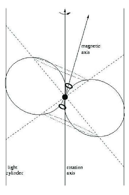
Figure 2: The emission geometry for pulsars at a low angle of inclination. Note that although the rings of nodes both near the pulsar surface (dark ring) and their mirrors on the null surface (finely dotted ring) encircle the magnetic axis, only the mirror ring also includes the rotation axis. The dotted straight lines representing the null surface separate negatively and positively charged regions of the magnetosphere, and their intersection with the last closed field-line defines the site of an “outer gap” [see Wright (2003a) for details].

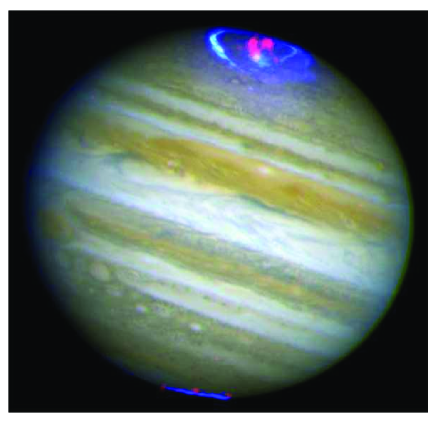
Figure 3: A multi-frequency image of Jupiter taken from the Chandra website. The (blue) UV ring and the (red) X-ray spots are superimposed on the well-known optical image. It is thought that the X-rays must originate from particles reflected from pole to pole. In the movie from which this picture is taken the intensity of the spots varies on the timescale of the interpole travel time. Image reproduced with kind permission from…

The promise of this approach is that such a feedback model has within it the capacity to explain more complex phenomena than the simple steady circulation of an axisymmetric system. As the magnetic inclination of a pulsar increases (while yet retaining near dipolar geometry at relevant heights), the system naturally causes the emission in the circulating “carousel” to develop a patchiness and asymmetry reminiscent of many observed features. In this view, the subbeam “carousel”, although always possessing a near-circular form, is no more than a distorted “reflection” of the outer-gap nodes, which circulate in tandem with those above the polar cap in an extended quasi-elliptical path about both the rotation and magnetic axes (Fig. 2). Although no time dependence is built into it, the model bears a striking resemblance to auroral models in terrestrial and planetary magnetospheres [comparisons with the recently discovered “drifting” x-ray hot spots around Jupiter’s poles (Gladstone et al. 2002—see Figure 3) are particularly apposite], and one may speculate that phenomena known from these fields—such as flares and magnetic reconnection—may be found to play an analogous role.

Core Emission

Core emission, as its name suggests, is emission which appears to be propagated in a narrow pencil beam surrounding the magnetic axis. Its angular dimensions are such that, if deemed to be coming directly from the polar cap surface, it would fill exactly the area enclosed by the “feet” of the last closed field lines. A great mystery, of course, is the relationship between this and the drift emission often found in the surrounding cones. We understand the gross distinctions between them in terms of their beam topology and modulation characteristics (ETI–V), but we understand virtually nothing about their commonality; and if the magnetosphere is truly operating as an integrated system, it seems most likely that both types of radio emission stem from the same sets of accelerated charged particles. It is tempting—yet at present no more than a speculation—to see at least a part of the core emission simply as the radial reflection of the emission of cascading downward flowing particles (Michel 1992; Wright 2003a). Such particles are an important component of the feedback model, and will certainly be powerful emitters as they are accelerated immediately above and towards the polar cap. Above all they will move down the last closed field lines from the outer gap and naturally define the limits of the polar cap.

Support for the interdependence of core and conal radiation comes from pulsars such as B1237+25, where our sightline runs almost directly over the magnetic axis. In the single pulse trains of this pulsar, the core region is dormant while the outer components have a strong and regular periodicity, but when the core brightens (as it does on quasi-periodical timescales) the conal modulation is interrupted, and only recommences when the core subsides (Hankins & Wright 1980). A case could be made to view the core emission from all pulsars as generally being inhibitive to regular periodicity in the conal components. This is certainly supported by observations of the well known pulsar B0329+54 (e.g., Bartel et al. 1982; Suleymanova & Pugachev 1998, 2002; hereafter SP98, SP02), which has multiple cones as well as a dominant central core component, yet has never been reported to show any periodic behaviour.

Surprisingly, core emission has still not been well studied. In part this is because it was identified after the heyday of enthusiasm for single-pulse investigations. It is also an unfortunate coincidence that most of the bright exemplars of core emission lie outside the declination limits of the Arecibo instrument. This is only a part of the story, however: the Vela pulsar, perhaps the prime example of core emission in the sky, has to date been poorly studied. No current well measured set of profiles is available, and we do not know if the star exhibits either polarization or profile modes or if it ever nulls. Many other things have been studied about this nearly unique and remarkably influential star (e.g., Krishnamohan & Downs 1983; Radhakrishnan & Deshpande 2001; Johnston et al. 2001; Kramer et al. 2001), but many of the basics remain a matter of guesswork.

The Vela pulsar B0833–45 is probably an excellent example of the core-single ${\bf S}_{\rm t}$ class—those with a single core component at meter wavelengths. ETIV has shown that it lies at the short-period end of a group whose component widths scale as $P^{-1/2}$—just as does the angular width of the polar cap. As the rotation period $P$ increases, there is a tendency for stars first to acquire an inner cone, and later an outer cone (ETVI). One might therefore suggest that as pulsars slow and lose their outer-gap high-energy emission (and by implication their capacity to create self-sustaining pair production here), sporadic low-energy pair-creation at either limit of the outer gap may still be permitted, and this in turn could generate conal radio emission through the feedback mechanism outlined above (Wright 2003a). As the pulsar further slows, these limits will become inaccessible to the sustaining surface x-rays, leading finally to the extinction of first the inner and then the outer cone.

This picture, again based on geometric argument, corresponds well to the observational analyses of ETI–VI. It also creates, yet again, the possibilty of a feedback system: when pair-creation becomes prolific in the outer gap, the downward-moving particles quench the potential and polar cap pair creation needed for conal radiation (Cheng et al. 1986). This reduces the heating of the polar cap, which therefore cools until its thermal x-rays cannot support the outer-gap pair avalanche, and the mechanism for creating conal radiation can recommence. Thus, the core emission can be seen as one component of a thermostatic process!

On the evidence above, the core emission is a very large and significant piece of the pulsar-emission jigsaw puzzle. In our future research we therefore should set about answering a series of guideline questions:

• How can we test whether the appearance of a core component in the radio emission is evidence of the onset of (possibly short-lived) runaway pair-creation in the outer gap? Some kind of statistical test for quasi-chaotic behaviour may be appropriate.

• Does the core component have significant structure within itself? If the conjecture of Wright (2003a) that core emission is in part reflected conal emission is correct, then the core structure may mimic the conical structure of the outer components. Such structure does seem to occur in B0329+54 (SP02), but in faster pulsars it is often difficult to discern whether the observed structure (Crawford et al. 2001) is to be interpreted as truly core or conal.

• If core activity is responsible for disrupting quasi-periodic conal modulation, can we detect this in the conal emission of pulsars which do not have a central sightline traverse? How do the statistics of periodicity loss in pulsars with only conal emission compare with those where the core is visible? These questions are clearly related to the phenomenon of moding, discussed in the next subsection.

• How common is quasi-periodicity in core components? And whether periodic or not, can any pattern of rise or fall or non-stochastic behaviour be discerned?

Moding: Changes in Subpulse Patterns

Historically, this phenomenon has often been associated with, and identified through, discrete variations in the profile shape. It was first identified by Backer (1970) in B1237+25, but later in a wide range of pulsars including B0329+54 (Lyne 1971, SP98, SP02), B1822–09 (Fowler et al. 1981), B2319+60 (Wright & Fowler 1981a), B0943+10 (Suleymanova & Izvekova 1984; Sulemanova et al. 1998; DR01) and most recently B2303+30 (Rankin & Wright 2003). Moding may well be universal, especially now that even B0809+74—long a considered a bastion of near-steady regularity (Lyne & Ashworth 1983)—has been shown to have a second mode (van Leeuwen et al. 2002). This effectively means that no well studied pulsar has been found to be free of moding.

However detected, moding is always associated with changes in the subpulse pattern. In those exemplars listed just above, the moding is easy to identify through clear and sudden changes in the profile shape. In others, such as B0031–07 (Huguenin et al. 1970) and B1944+17 (Deich et al. 1986), the mode change is seen as an immediate and significant change in subpulse drift rate, with later analysis then revealing an associated profile change (Wright & Fowler 1982). The changes are often easy to identify, but in some prominent pulsars exhibiting profile moding without any regular subpulse modulation (e.g., B0329+54), it is important to identify what changes in the PSs correlate with the mode changes, work already well started by Suleymanova & Pugachev (SP98, SP02).

Interestingly, it seems that at least some pulsars “anticipate” their mode changes. This has been demonstrated in both B0329+54 (SP98; SP02) and B0943+10 (Suleymanova et al. 1998) where subtle intensity variations begin some hundreds of pulses before the more dramatic—almost instantaneous—mode change actually occurs. It is curious (and hard to account for theoretically) that this slow anticipatory modulation does not seem, in the case of the exquisite “drifter” B0943+10, to affect the periodicity of its drift. Work is underway to see if B2303+30, which in many ways resembles B0943+10 but whose mode changes are more frequent, also shares this property.

On the basis of these observations it may be useful from a theoretical standpoint to distinguish between two types of modes: “ordered” modes in which the subpulses exhibit regular behaviour such as drift, and “disordered” modes, where the emission is predominantly chaotic. Thus, B0031–07 and B1944+17 have three modes of the first kind, B0809+74 (van Leeuwen et al. 2002) has at least two of the same, B1237+25 one of each, and both B0943+10 and B2303+30 may have several ordered and one disordered mode (Rankin et al. 2003; Rankin & Wright 2003). Often the changes between the ordered modes may be gradual, as in B2016+28 (Oster et al. 1977).

In most of the pulsars with more than two ordered modes, it has been found that mode changes do follow some systematic “cycle” (generally accelerating the drift rate through increasing values before returning to the “start”). Examples are B0031–07, B1944+17 and B2319+60, and this may well be a common feature at least of slow-drift pulsars. This apparent memory is a powerful clue and we must learn how to interpret it (see the Emission Cycles section below).

In pulsars with “disordered” modes, we must ask if this might always correspond to the onset of core emission, even if that emission is fortuitously invisible to us. This question is closely related to our discussion of B1237+25 in the previous section. The apparently spontaneous switching from one emission mode to another, whether ordered or not, is, of course, the hallmark of a quasi-chaotic system. It need not imply that the switch is “caused” by any external agency either from the interstellar medium or the neutron star crust. Nor need the moment of change be at all predictable. Nevertheless, time series generated from these changes may not be entirely chaotic and it may be possible to borrow analytical techniques from studies of non-periodic phenomena in other fields to mine underlying information about the physical system which produces moding.

Our understanding that the integrated profile forms are produced by a system of circulating subbeams, which is highly symmetric about the magnetic axis, constrains our possible interpretations. When a mode change occurs between ordered modes, it is crucial to know which parameters have concurrently changed. It was originally believed—for example in the case of B0031–07—that the repetition rate $P_{3}$ altered suddenly, but that the driftband separation, $P_{2}$, remained unchanged. This would imply geometrically that the emitting regions, and their corresponding nodes, would remain on the same fieldlines but accelerate their drift motion. This appears to be true, at least to first order, for the five or six pulsars where this phenomenon is known. Some doubt was cast on this by the discovery that the profiles of the successive modes did actually widen (Wright & Fowler 1982), a result later confirmed by Vivekanand & Joshi (1997). These latter authors further claim that their driftband measurements suggest significant increases in $P_{2}$ from mode to mode (i.e., as $P_{3}$ decreases). Such measurements are notoriously difficult to make, not least because $P_{2}$ varies across the pulse window and may be subject to polarization and “absorption” effects (see next section). However van Leeuwen et al. (2002) identify a similar effect in B0809+74, where an increase in $P_{3}$ is associated with a narrowing profile and an increase in $P_{2}$.

If confirmed, the change in $P_{2}$, though slight, would imply (pointed out by van Leeuwen et al. 2002) that the emission beam has rapidly moved radially across fieldlines, and in terms of our geometric model here this would mean the outer gap nodes would have migrated to different latitudes on the outer gap and the polar nodes to new radii on the polar cap. This is perfectly possible (given that we do not know the nature of the underlying cause for the mode change!) and would reveal interesting properties for the model, but it is first necessary to confirm this result in more detail: again, it is the observations which must be the arbiter of the form the model takes.

Nulling

“Null” pulses are identified by a complete absence of intensity throughout the entire pulse window, and appear to interrupt pulse sequences without warning. Often they persist for many periods (some pulsars are known which remain in a “null” state most of the time), and then emission reappears as suddenly as it ceased. The phenomenon is more common in older, longer-period pulsars, although it is no longer believed that pulsars “die” through gradually “nulling away” (see ETIII). In certain pulsars nulls and subpulse drift have long been understood as closely associated (Unwin et al. 1978; Filippenko & Radhakrishnan 1982; Lyne & Ashworth 1983), but we still have remarkably little physical understanding of these nulls.

It is possible that there are several different kinds of nulls (see Backer 1971), an idea also hinted at in analyses of the slow-drifting, moding pulsar B0031–07 (Vivekanand 1995), who found a bimodal distribution of null length. Vivekanand did not, however, identify where the two types of nulls occurred in the PSs. It is very possible that the shorter nulls tended to occur within a single mode (i.e., the mode persists following the null) and that the longer “nulls” occurred between different modes. One might also take B0809+74 as evidence for this idea, as its slower drift mode(s) always seem to follow long null intervals (van Leeuwen et al. 2002).

By contrast, in fast-drifting pulsars there are now strong indications that nulls are associated with subbeam circulation in a broader context: pulsar B2303+30 rarely seems to null when in its bright and well ordered drift mode, but it exhibits deep nulls in PSs which are less orderly or chaotic (Rankin & Wright 2003). Pulsar B0834+06 exhibits mostly 1-pulse nulls which appear to fall on the weak phase of its nearly even-odd PS modulation. Can it be that in a pulsar (e.g., B1133+16) with sporadic pulse-to-pulse modulation, there are occasionally “empty” sightline traverses through the average emission-beam pattern which simply fail to encounter significant radiation? In order to answer such questions, new investigations of pulsar nulling are required which investigate the link between nulling and subpulse behaviour.

A recent result of this new approach is the success in understanding the null/drifting interaction in B0809+74. van Leeuwen et al. (2002, 2003) have shown not only that each transition to the second mode is preceded by a null sequence, but that during every null sequence the phase of the subpulse is “remembered” and then gradually accelerates either to its previous mode or a new mode. This is a more subtle interaction than previously suspected (Lyne & Ashworth 1983).

Knowing the source and growth of nulls in the magnetosphere would give great insight into their nature. The onset and ending of a “null” are so rapid that they are hard to catch in the moment—though such a population should occur statistically in many pulsars. We do not know how close to simultaneous is the onset at different frequencies (and by implication at differing locations in the emission zone), nor whether it ends as fast as it commences. Currently the Multi-Frequency, Multi-Observatory Pulsar Polarimetry (MFO) Project (Ramachandran 2002) is gathering simultaneous broad-band observations which are providing the first general opportunity to address such questions. Does the entire “carousel” of subbeams switch off together? A study of nulling in conal double (D) pulsars might help resolve this. From an observational point of view it is difficult to distinguish between short “nulls” (with absolutely no emission) and very weak emission, so the observations required are not easy to obtain.

The statistics of null and burst length in a given pulsar are as important as the null fraction. Where null pulses occur within PSs is equally crucial. An interesting analogy to nulling—and to mode changing too—is the incidence of terrestrial earthquakes or avalanches, where larger earthquakes (avalanches) occur less frequently according to a specific law (the Gutenberg-Richter law). It is known that statistics of these “self-ordered critical systems” (SOC’s) reveal characteristics of the underlying physical processes, typically through the presence of power-law distributions (Bak 1996). This procedure has also successfully been applied to solar flares and magnetic reconnection, and would be interesting to pursue in this context.

There are virtually no working theories which adequately account for nulling, and hence there is no agreement as to whether nulling occurs because the engine producing the emitting particles temporarily “switches off”, or whether the emission process itself breaks down. For example, in the feedback model outlined here, the flow from the suface to the null line and back may not be continuous and may contain irregular or even “void” stretches of low particle density creating voids in emission, which we experience as nulls. Alternatively, or additionally, nulls may arise through a breakdown in the mechanism which maintains the coherent radiation. This latter could arise simply because the rapidly changing flow cannot hold the flow steady enough for the conditions producing coherence to develop. Thus the nulling phenomenon could be seen as the visible yet ‘superficial’ response to one of a range of deeper underlying conditions. One might then predict that nulls will be more prevalent in highly irregular stretches of emission, and there is some suggestion of this in the observations of a number of pulsars (e.g., B2303+30), but it is important to test this in more careful analyses of observations.

Emission Cycles

In a number of pulsars, so far 4, the emission modes are characterized by a progressive increase in drift-rate through at least 3 modes. These pulsars [B0031–07 (Huguenin et al. 1970), B1918+19 (Hankins & Wolszczan 1987), B1944+17 (Deich et al. 1986), B2319+60 (Wright & Fowler 1981a)] all have very low drift-rates in their principal modes, and the magnetic axes of all are thought to be weakly inclined with respect to their rotation axes.

What is remarkable about them is that the mode sequences appear to follow certain “rules”. For example, B0031–07 has 3 identified modes, A, B and C, which have repetition periodicities ($P_{3}$s) of about 12, 8 and 5 periods respectively. These modes are interspersed by null stretches, both within a mode and between modes. But often a mode-change occurs without an intervening null, and then it is found that only transitions A to B or B to C are allowed (Huguenin et al. 1970; Wright & Fowler 1981b). The transitions take place within a few rotation periods at most, possibly within a single period. In other words, sudden, null-free mode changes in which the driftbands retain their identity can only occur when the mode change corresponds to an increase in the drift rate. This gives the impression that the pulsar emission is executing a kind of cycle, from A to B to C, which may last some hundreds of pulses. Not all cycles include C, which is anyway of short duration.

These properties are shared by the remaining 3 pulsars, and recently the pulsar B0809+74, also with a slow drift rate and low inclination, has also been shown to have smooth transitions (preserving drift-band identity) from a slow mode to fast, but only fast to slow following a long null (van Leeuwen et al. 2002). All this suggests that the subpulse sequences possess direction, even “memory”. This behaviour is known in many branches of non-linear studies. Near-chaotic systems can move from one pattern to another, apparently unpredictably, migrating from one limit cycle to another with a corresponding change in attractor. Regarding profiles as attractors, this is precisely what the changing pulsar profiles reveal: the profiles of the emission modes do seem to widen as the driftrate increases, and by a similar amount in each pulsar.

A further curious fact about these pulsars is that the ratios of their successive modal drift rates are about the same: all (including B0809+74) appear to increase their driftrates by about 1.6 as they move from one mode to the next. Whether this increase entirely stems from a reduction in the pattern repetition rate ($P_{3}$), or whether also the band spacings ($P_{2}$) are slightly reduced [as Vivekanand & Joshi (1997) and van Leeuwen et al. 2002 find for B0031–07 and B0809+74 respectively] is important to clarify.

It is fascinating to speculate as to what is physically happening during these “cycles”. It seems unlikely that additional nodes (Wright 2003a) or sparks (Gil et al. 2002a,b; Gil & Melikidze 2002) are created as the mode transitions occur, for they seem to be smooth and no act of node/spark creation is observed. The conclusion is that the emission region, and hence the nodes/sparks, must migrate radially to an inner set of field lines. In Wright’s model, the outergap mirror points must move along the gap further from the star. The cycle would then begin with a slow drift in outer fieldlines, possibly those bounding the corotating zone, and progress towards the axis. This spiral inwards is reminiscent of the model suggested many years ago for B1237+25 by Hankins & Wright (1980), although in this strongly inclined pulsar the entire sequence lasts only 2.8 periods. Note also that the slow drift rate of the weakly-inclined pulsars implies (in the model of Wright 2003a) that the outergap nodes are nearly corotating with the star—appropriate to the corotating zone boundary. Then, as the modes progress, they spin faster (in the corotating frame) counter to the rotation of the star, and eventually become closer to being stationary in the observer frame and nearer the light cylinder.

The fact that we have only 4 established examples so far of this cyclic behaviour may be because lengthy and detailed studies of the subpulse sequences is necessary before the mode-change “rules” become apparent. But if subpulse behaviour does result from magnetospheric feedback (Wright 2003a), it also may be because at the more common larger angles of inclination (say between 20^∘ and 50^∘) the structure of the magnetosphere’s potential becomes highly asymmetric, with both faster driftrates and more blurred mode changes. Hence slow long-term cycles may only be a feature of nearly-aligned pulsars.

Integrated Profile Questions or Attractor Analyses

Although we have stressed the importance of single pulse analyses and implied that they are the true currency of a pulsar’s emission, the fact remains that single pulse analysis is only possible for a small minority of the pulsar population. Only 10–20 pulsars have so far had their single pulse behaviour documented, and for some of these the description is only preliminary [e.g., B1112+50 (Wright et al. 1985)] or relatively inaccessible (e.g., Ashworth 1982; Backer 1971). Many more bright pulsars, some recently discovered (e.g., Lorimer & McLaughlin 2003), are deserving of greater study and we feel a major effort should be made to accelerate their analysis.

We are therefore forced to accept that for the majority of pulsars (there are some 1700 known to date) only their integrated profile is available for study. Yet, so long as we continue to bear in mind their nature as attractors, it is possible to mine a great deal of information, particularly of a geometric nature, from this population. This is essentially what was done by one of us (ETI,ETII,ETIII) and Lyne & Manchester (1988) in the eighties, when perhaps 200 usable profiles were available.

What now needs to be done is to look at these results in the light of our twin hypotheses of nearly circular subbeam circulation, and a pan-magnetosphere feedback system. We will take in turn a number of crucial aspects of profile analyses, and pursue the consequences.

Double-Cone Beam Structure

While several pulsars with five distinct components had long been known (e.g., B1237+25, B1857–26), suggesting two conal rings as well as a central core beam, it was not until 1993 (ETVI) that firm evidence was given for two cones with coherent geometrical characteristics (then confirmed by Gil et al. 1993; Kramer et al. 1994). Specifically, the respective inner and outer cones in double-cone (M) stars were found to have outside, half-power, 1-GHz radii of 4.33${}^{\circ}P^{-1/2}$ and 5.75${}^{\circ}P^{-1/2}$—and the single cones of triple (T) pulsars were found to be one or the other. Then, ETVII showed that while outer cones exhibit RFM, inner-cone radii appear to be nearly constant over the entire radio band.

It is still not understood why some pulsars have two concentric cones and what is the relation of the subpulse modulation in the two cones. Even for the paragon of this phenomenon, B1237+25, there is very much still to learn. One line of approach has assumed that double-cone emission probably comes from the same set of emitted charges, whether sparks or beams (e.g., Deshpande & Rankin 2001), while Gil and collaborators (Gil & Sendyk 2000; Gil et al. 2002a,b; Gil & Melikidze 2002) have envisioned several concentric rings of sparks on the stellar surface which are thought to be associated with the various cones and even the core. The implications of these assumptions are very different, and almost no work has been devoted to pursuing their study through PS analyses. There are now almost 20 stars with well identified double-cone profiles (see ETVI), so a systematic study is possible and feasible—though perhaps no more than half a dozen are strong enough for PS analysis. In any case, that rotating subbeams are responsible for the generation and modulation of these cones gives us new ways of studying and assessing their character and origin.

RFM/no RFM

The phenomenon that prominent conal double profiles (e.g., B1133+16) become progressively wider with wavelength was well noted very early (Komesaroff 1970), and many workers participated in documenting the effect, often by fitting pairs of power-law functions to the asymptotic high and low frequency profile widths or component spacings (e.g., Lyne et al. 1971; Sieber et al. 1975). Thorsett (1991) demonstrated that a function of the form $\varphi_{0}$+$(f/f_{0})^{-a}$ fitted the full low to high frequency behaviour well. von Hoensbroech & Xilouris (1997) have provided a full review of work on “radius-to-frequency mapping” (hereafter RFM) in the course of extending the range of the high frequency observations.

The question of RFM has perhaps become more interesting with the conclusion that it is exclusively a characteristic of outer-conal beams (Mitra & Rankin 2002; ETVII). This study included the beam geometry for the first time, so that conclusions are framed in terms of conal beam radii and emission heights. In addition, two different types of RFM behaviour were identified among the outer cones—those which approach a constant radius at the highest frequencies and those that do not.

Nonetheless, in many other ways the emission from inner and outer conal beams is indistiguishable, so that it again becomes a question of how a rotating subbeam system radiates in such a manner that its envelope does or does not exhibit a frequency dependent radius. Closely related questions arise in considering the significance of the altered profile forms produced by mode changes. This was first noted in the context of pulsar B0329+54 (Lyne 1971), but excellent examples are now also B0611+22 (Nowakowski & Rivera 2000) and recent studies of B0809+74 (van Leeuwen et al. 2002, 2003).

The problem is aggravated by the fact that there is no agreed model for the production of emission. Assuming that the coherent radiation is emitted tangentially to field lines in the polar cap region some hundreds of kilometers above the stellar surface, the critical problem is then to determine precisely which fieldlines are carrying the emission and at which height (Kijak & Gil 2003). This is no easy task given the likely effects of aberration and time-delay (Gangadhara & Gupta 2001; ETVII). From the standpoint of the feedback model, this work is very important, since it will determine the nature and true positioning of the link to the outer gap.

“Absorption”

This phenomenon relates to the gross asymmetry which is evidenced in certain pulsar profiles, yet only within certain frequency ranges, suggesting that the asymmetry is not an intrinsic property of the profile but that some intervening medium has partly “absorbed” the emission. Although first discussed in the context of multi-frequency alignment anomalies in the relatively stable pulsar B0809+74 (Davies et al. 1984; Bartel et al. 1981; Bartel 1981), where the drifting subpulses become blurred and attenuated as they pass through a specific longitude. range. The phenomenon is now also known to be closely associated with profile mode changing, as (e.g., in B0943+10) the degree and character of the “absorption” is strongly correlated with the profile mode. Thus much of what was said above in regard to profile modes is equally applicable here. Indeed, perhaps profile-mode changing and “absorption” should be viewed together as two faces of one phenomenon—the temporal and profile-spectral manifestations of a single cause which is also manifested in the PS pattern. From an observational standpoint we now can see why “absorption” is most clearly or usually identified in pulsars with $|\beta|$/$\rho$ near unity (i.e., usually stars which are members of the ${\bf S}_{\rm d}$ profile class) whereas profile mode changing is most easily identified in multiply-peaked pulsars with $|\beta|$/$\rho$ much less than unity.

A more recent variation of this topic has come with the discovery of mysterious “notches” in the profiles of a number of very different pulsars (McLaughlin & Rankin 2003). These are found in certain wide-profile pulsars, are narrow double-dip in character, and tend to follow the profile centroid by about 60^∘ longitude. The critical question is whether they are intrinsic to the profile or are truly absorption. There is a need for frequency-dependent studies to resolve this, since if not intrinsic the notches could for the first time identify very localised regions of the magnetosphere where the absorption takes place.

Defining the location of absorption, given the geometric theme of this paper, is something of a challenge. Assuming that the effect is not occuring within the circulating subbeams, we have to track the likely path of the radiation as it escapes the magnetosphere. Three things will be crucial to this: 1) the longitude in the profile, which defines the moment and angle of emission, 2) the rotation period, which fixes the scale of the magnetosphere, and 3) the angle of inclination, which locates the position of the null surface, the outer gaps and the distance from the magnetic pole to the light cylinder.

A start on this problem very much in keeping with the “keep-it-simple” geometrical ideas of this article has recently been made on the issue of profile notches: it can be shown that if, as generally assumed, the emission frequency is height-dependent, then double-notches can arise through time-delay and aberration in quite natural geometries and needs no appeal to “distorted” field-lines (Wright 2003b).

RF Spectra, Rotation Energy Loss & RF Efficiency

That conal beams are produced by systems of rotating subbeams gives us the possibility of estimating the full radiation pattern of a given pulsar in terms of what we observe in the course of our particular sightline traverse. A first effort in this direction was made by Deshpande & Rankin (1999) for pulsar B0943+10. Then, the emission from the full beam pattern at a given frequency can be integrated over the pulsar’s full spectrum and compared with its rotational energy loss to estimate its overall RF radiation efficiency. Such efforts, carried out for a substantial group of stars promise to provide an important quantitative point of connection with physical theories of pulsar emission.

The above work depended on low frequency observations made over many years at the Pushchino Radio Astronomy Observatory and the catalogues of pulsar spectra and luminosity estimates compiled by Malofeev and colleagues there (e.g., 1996, 1999). Otherwise, only limited progress has been made in understanding why pulsars exhibit different radio-frequency spectra. Some attention has been paid to spectral-index differences at centimeter wavelengths (i.e., Maron et al. 2000) as well as the breaks in such indices exhibited by certain stars (Ochelkov & Usov 1984; Beskin et al. 1988; ). However, equally important is the issue whether a pulsar’s spectrum turns over at low frequencies (Benford & Bushauer 1977; Malofeev & Malov 1981). Some pulsars (e.g., B0329+54) exhibit spectral turnovers at 100–300 MHz, and thus are observable at low frequencies only with great difficulty, if at all. Other pulsars—and it seems all of those best known for their regular drifting-subpulse systems (e.g., B0031–07, B0809+74, B0943+10)—are observable to very low frequencies. B0943+10 in particular exhibits no spectral turnover down to some 30 MHz (Deshpande & Rankin 2001). It should thus now be possible to gain some insights into the physical reasons for such different behaviours.

Emission Questions

Microstructure and Giant Pulses

A number of observations and developments have begun to narrow the possible interpretations of microstructure. Apparently, the fine temporal structure of microstructure has been resolved, and additionally there is evidence that its autocorrelation length scale is roughly proportional to the pulsar period (Popov et al. 2002). Observations using the Effelsberg and Westerbork instruments seem to show in pulsars like B0329+54 that micropulses occur in all three main components (Lange et al. 1998; Ramachandran 2001) so that the phenomenon—as with nulling—affects both core and conal components. It is, however, far from clear what connection, if any, micropulses have with subbeams in S_d stars such as B0809+74 or whether there is any orderliness to their polarization characteristics. Much work then needs to be done in order to assess how closely associated microstructure is with the other primary pulsar phenomena—and the study of microstructure in a pulsar with a very orderly rotating subbeam system such as B0809+74 undoubtedly has much to teach us about the nature of microstructure.

In a small, but now growing, number of fast pulsars microstructure is found to be associated with the phenomenon of “giant pulses”. Such pulses are narrow but exhibit an intensity far in excess of the mean pulse energy. They were first found in the Crab pulsar (Heiles et al. 1970; Lundgren et al. 1995; Hankins & Kern 2003), but recently have also be found inspun-up millisecond pulsars (e.g., Kinkhabwala & Thorsett 2000). Theyhave a distinctive power-law energy distribution—possibly suggestive of self-organised criticality (see earlier section on Nulling, and Young & Kenny, 1996), suggesting they might be the response to a simple generating physical system operating on a wide range of scales in a self-similar manner. Furthermore, they often occur at phases close to those of the high-energy profile components (Romani & Johnston 2001). Assuming high-energy emission is indeed emitted from outer gaps, all this intriguingly hints at an independent physical radio source for giant pulses and at an interrelationship between polar cap and outer gap radio emissions.

Polarization Issues

The origin of the orthogonal polarization modes (OPM) is one of the great mysteries of the pulsar emission problem. Those stars so far well studied in terms of their OPM characteristics are so far almost all conal dominated, so we have virtually no good examples apart from B0329+54 (Bartel et al. 1982; Gil & Lyne 1995; SP98, 02) of core components that can indicate what role the OPM play in core emission. What is increasingly clear is that conal pulsar beams are highly modal in their angular beaming characteristics (Deshpande & Rankin 2001; Rankin & Ramachandran 2003; Rankin et al. 2003). OPM has historically been assumed to be a characteristic of the pulsar emission mechanism, but there is now theoretical work to the effect that it may result from propagation effects (Arons & Barnard 1986; Petrova 2000). Basic questions about whether the two modes occur simultaneously in individual samples and whether they are fully or partially polarized remain. The issue of how such characteristics vary with frequency, and whether they might be implicated in the general lower levels of polarization at very high frequencies, has only been touched. Again, each of these questions can fruitfully be studied in the context of a rotating subbeam system, because the modulated character of the signals gives one an additional method by which to separate the combined effects of the modal interactions. The work of McKinnon & Stinebring (1998, 2000) has provided a much sounder statistical and interpretive foundation for OPM work, but analyses based on sensitive and fully calibrated recent observations are needed to carry this work further.

Just why pulsars have polarization and depolarization remains a mystery. The modal character of the rotating subbeam systems which produce conal beams is probably almost entirely responsible for the complex variety of characteristics observed in different pulsars with conal profiles. Rankin & Ramachandran (2003) have explored the character of this beam-edge depolarization in stars with conal components pairs where our sight-line passes close to the magnetic axis as well as in conal single (${\bf S}_{\rm d}$) stars where our sightline makes an oblique traverse, finding that a virtually identical beam configuration can produce the full range of observed effects. Therefore, it should be possible to model the depolarization of the conal emission in a wide variety of situations to both improve our knowledge of the conal emission geometry as well as the nature of the modal emission which produces the polarization and depolarization. This is a rich area for immediate study and a good example of how the context for PS analysis and interpretation has been changed almost completely by our expectation that rotating subbeam systems produce the emission which both polarizes and depolarizes conal components.

A closely related question is the polarimetric relation between inner and outer conal beams. We often see evidence for two active modes on the outer edge of the emission beam and only one in interior regions of the profile (or beams). In a double-cone star (e.g., B1237+25) this means both modes are active in the outer cone, but only a single mode is apparent in the inner cone. However, we also see cases of inner-cone D or T stars where both modes are also active in their inner cones. Must this circumstance not bear importantly on how the OPM is generated—that is, whether it is an emission or propagation effect?

X-ray, Optical & $\gamma$-ray Emission

We close our carousel of pulsar phenomenology (Fig. 1) with a discussion of high-energy pulsar observations and their relation to the radio emission.

Although nearly 2000 radio pulsars have now been discovered, only a handful of these have been detected at high-energy wavelengths. Future satellites promise to greatly expand this number, but there remains a feeling that we are dealing with two classes of pulsars: one population where the x-ray and shorter wavelength emission is closely correlated with young pulsars having large values of $B_{12}/P^{2}$ together with prominent or exclusive core emission beams at radio wavelengths, the other with no high-energy emission and exhibiting predominantly conal features. The contrast is exacerbated by the fact that pulse-sequence analysis is still impossible for the high-energy emission, and that therefore only profile (i.e., attractor) studies are available. This has further fostered the impression that such pulsars are in a steady state, and furthermore emit from different regions by a different mechanism.

Yet this dichotomy may be an illusion, brought about simply by the differing means by which the high-energy and radio emisson are detected: a major point stressed in Wright’s (2003a) work is that even in slow pulsars the radio emisson may require the interactions between differing regions of the magnetosphere. Thus a highly-energetic pulsar with core emission and an old pulsar with only outer cone radio emission above the level of detectability represent opposite ends of an evolutionary spectrum. Younger pulsars with energetic outer gaps would “quench” the electric field in the conal regions above the poles (Cheng et al. 1986), and the downflowing particles would somehow generate the core emission, possibly by reflection of incident radiation generated just above the polar cap surface.

Measurements of correlations between core and high-energy emission must become possible in the near future and provide an opportunity to test and develop these ideas. For example, certain x-ray pulsars, such as B0611+22 (Nowakowski & Rivera 2000), exhibit slow quasi-periodic profile changes which could be interpreted as a very slow rotation of one or more subbeams (Kern 1998), and it would be interesting to know whether the x-ray emission is modulated or correlated with these radio profile variations.

The evolutionary picture has received some theoretical support from the recent studies by Harding and her coworkers (Harding et al. 2002; Harding & Muslimov 2002a,b) of pair creation in the polar cap region. Building on the earlier work of Hibschman & Arons (2001a,b) which incorporates the effects of backflowing particles in determining the height of the acceleration zone, they envisage a pulsar’s radio emission as a two-phase process: above the polar caps of young pulsars the principle radiation mechanism by which pairs are produced is curvature radiation, which generates sufficient pairs to screen the ambient electric field. However in older, “slow” pulsars, this gives way to radiation dominated by inverse Compton scattering—and crucially the electric field above the acceleration zone cannot now be fully screened. This implies that particles will continue to be slowly accelerated towards the outer gap, where Wright (2003a) envisages the occurence of further pair creation. Intriguingly, Hirotani & Shibata (2001) have recently shown that the precise location of the outer gap will itself depend on the inflow and outflow of current, suggesting further non-steady feedback processes. The implication of these exercises is that we ignore interactions between the polar cap and outer gap at our peril.

Conclusions

This paper represents an attempt to take a novel view of the pulsar phenomenon. By abandoning the view that a pulsar’s magnetosphere is in a near-steady state, and further that its behaviour on all scales of time and space is determined by so far unexplained, yet complex events on the tiny polar caps, it is argued that a promising new approach is possible.

Thus the magnetosphere is seen as having an inclined, essentially dipolar, structure, whose apparently complex emission arises not from abitrarily complex magnetic field components, but from subtle time-delayed interactions between regions relatively remote from one another. The principle interaction exists between the magnetic polar regions of the neutron star and the outer gap. But it is also arguable that, quite possibly, a similar aurora-like mirror interaction occurs between the poles—a feature which might be mathematically represented as a particle “pressure” exerted within or at the surface of the closed corotating “dead” zone (Mestel et al. 2003). Each region of the magnetosphere is then dependent on every other, yet never in a steady state and always with a natural time lag. This idea is distinctly different from the more conventional view that the flow is driven smoothly from the tiny polar regions to the light cylinder, and opens a whole new line of pulsar investigation.

In developing our specific ideas we lean on both the observational analyses of one of us (ETI-VIII) and the recently developed concepts of the other (Wright 2003a), where the geometry of the feedback process has been examined in greater detail and successfully compared with observations in a few highly-organised pulsars. Such a feedback system can naturally proceed to bifurcations (i.e., alternate states) and ultimately to fully chaotic emission without any need to invoke strange geometries or external influences. This behaviour is highly reminiscent of what is found in real pulsars, and thereby hints at the possibility of uniting theory and observations.

Here an attempt is made to link these new ideas to the principal long-standing conundrums found in the study of older, slow pulsars. But the wider purpose is to suggest that future theoretical investigations may benefit from links to existing studies of the properties of time-dependent non-linear systems, which demonstrate that highly complex behaviour can be found in even the simplest systems. Similarly, the subtle statistics of time series, often used to mine information from apparent chaos in fields far removed from astrophysics, might be usefully applied to pulsar sequence data. It would not be the first time that cross-discipline studies have given unexpected insights.