Varying Alpha in a More Realistic Universe

Abstract

We study the space-time evolution of the fine structure constant, $\alpha$, inside evolving spherical overdensities in a lambda-CDM Friedmann universe using the spherical infall model. We show that its value inside virialised regions will be significantly larger than in the low-density background universe. The consideration of the inhomogeneous evolution of the universe is therefore essential for a correct comparison of extragalactic and solar system limits on, and observations of, possible time variation in $\alpha$ and other constants. Time variation in $\alpha$ in the cosmological background can give rise to no locally observable variations inside virialised overdensities like the one in which we live, explaining the discrepancy between astrophysical and geochemical observations.

Recent observations of small variations in relativistic atomic structure in quasar absorption spectra murphy suggest that the fine structure constant $\alpha$, was smaller at redshifts $z=1-3$ than the current terrestrial value $\alpha_{0}=7.29735308\times 10^{-3}$, with $\Delta\alpha/\alpha\equiv\{\alpha(z)-\alpha_{0}\}/\alpha_{0}=-0.543\pm 0.116\times 10^{-5}$. Several theories of varying $\alpha$ have been proposed to investigate the implications bsbm . Time-varying $\alpha$ requires a scalar field that couples to electromagnetically-charged matter. Variations in $\alpha$, allowed by the conservation of energy and momentum will then depend on the expansion of the universe and the evolution of the electromagnetically coupled matter. The inclusion of electroweak or grand unification will create more complicated consequences and constraints lang . Variations in $\alpha$ due to perturbation in the matter fields were first studied in mota2 , using the linear theory of cosmological perturbations. It was shown there, that perturbations in $\alpha$ will grow during the matter-dominated epoch and will be constant or decay during the other eras. In otoole the effects of $\alpha$ on gravity were also analysed. However, any effects on the time and spatial evolution of $\alpha$ due to cluster and galaxy formation has been ignored in the literature. This is a major weakness and, as a result, past attempts to confront observations on extragalactic scales with lab or solar system constraints on $\alpha$ variation are all questionable. This letter describes the first attempts to follow the inhomogeneous evolution of $\alpha$ during the development of non-linear cosmic structures. We compare the evolution of $\alpha$ in the background universe and in overdense regions of the universe.

We will study variations in $\alpha$ in the Bekenstein-Sandvik-Barrow-Magueijo (BSBM) theory bsm1 , which assumes that the total action of the Universe is given by:

$$S=\int d^{4}x\sqrt{-g}\left(\mathcal{L}_{g}+\mathcal{L}_{m}+\mathcal{L}_{\psi}+\mathcal{L}_{em}e^{-2\psi}\right)$$ (1)

In the BSBM varying-$\alpha$ theory, the quantities $c$ and $\hbar$ are constants, while $e$ varies as a function of a real scalar field $\psi,$ with $e=e_{0}e^{\psi}$. $\mathcal{L}_{\psi}={\frac{\omega}{2}}\partial_{\mu}\psi\partial^{\mu}\psi$, $\omega$ is a coupling constant, and $\mathcal{L}_{em}=-\frac{1}{4}f_{\mu\nu}f^{\mu\nu}$. The gravitational Lagrangian is the usual $\mathcal{L}_{g}=-\frac{1}{16\pi G}R$, with $R$ the Ricci curvature scalar. $\mathcal{L}_{m}$ is the matter fields Lagrangian. Defining an auxiliary gauge potential by $a_{\mu}=\epsilon A_{\mu}$ and a new Maxwell field tensor by $f_{\mu\nu}=\epsilon F_{\mu\nu}=\partial_{\mu}a_{\nu}-\partial_{\nu}a_{\mu}$, the covariant derivative takes the usual form, $D_{\mu}=\partial_{\mu}+ie_{0}a_{\mu}$. The fine structure constant is then $\alpha\equiv\alpha_{0}e^{2\psi}$ with $\alpha_{0}$ the present value here.

The background universe will be described by a flat, homogeneous and isotropic Friedmann metric with expansion scale factor $a(t)$. Varying the total Lagrangian we obtain the Friedmann equation ($\hbar=c\equiv 1$) for a universe containing dust, of density $\rho_{m}$ $\propto a^{-3}$ and a cosmological constant $\Lambda$ with energy-density $\rho_{\Lambda}\equiv$ $\Lambda/(8\pi G)$:

$$3H^{2}=8\pi G\left(\rho_{m}\left(1+\left|\zeta\right|e^{-2\psi}\right)\ +\rho_{\psi}+\rho_{\Lambda}\right)$$ (2)

where $H\equiv\dot{a}/a$ is the Hubble rate, $\rho_{\psi}=\frac{\omega}{2}\dot{\psi}^{2},$ and $\zeta=\mathcal{L}_{em}/\rho_{m}$ is the fraction of the matter which carries electric or magnetic charges. The value (and sign) of $\zeta$ will depend on the nature of dark matter: $\zeta\approx 10^{-4}$ for neutrons or protons but $\zeta=-1$ for superconducting cosmic strings bsm1 . The scalar-field evolution equation is

$$\ddot{\psi}+3H\dot{\psi}=-2e^{{-2\psi}}\zeta\rho_{m}/\omega.$$ (3)

Variations in $\alpha$, due to the formation of overdense spherical regions, can be studied using the spherical infall model padmanaban . We model the spherical overdense inhomogeneity by a closed Friedmann metric and the background universe by a spatially flat Friedmann model. Each has their own expansion scale factor and time, which are linked by the condition of hydrostatic support at the boundary. This approach is equivalent to study the effect of perturbations to the Friedmann metric by considering spherically symmetric regions of different spatial curvature in accord with Birkhoff’s theorem. The density perturbations need not to be uniform within the sphere: any spherically symmetric perturbation will evolve within a given radius in the same way as a uniform sphere containing the same amount of mass. Clearly, this model ignores any anisotropic effects of gravitational instability or collapse. Similar results could be obtained by performing the analysis of the BSBM theory using a spherically symmetric Tolman-Bondi metric for the background universe with account taken for the existence of the pressure contributed by $\Lambda$ and the $\psi$ field. In what follows, therefore, density refers to mean density inside a given sphere.

Consider a spherical perturbation with constant internal density which, at an initial time, has an amplitude $\delta_{i}>0$ and $|\delta_{i}|\ll 1$. At early times the sphere expands along with the background. For a sufficiently large $\delta_{i},$ gravity prevents the sphere from expanding. Three characteristic phases can then be identified. Turnaround: the sphere breaks away from the general expansion and reaches a maximum radius. Collapse: if only gravity is significant, the sphere will then collapse towards a central singularity where the densities of the matter fields would formally go to infinity. In practice, pressure and dissipative physics intervene well before this singularity is reached and convert the kinetic energy of collapse into random motions. Virialisation: dynamical equilibrium is reached and the system becomes stationary: there are no more time variations in the radius of the system, $R$, or in its energy components. In the spherical collapse model, due to its symmetry, the only independent coordinates are the radius of the overdensity and time. Also, as is standard practice when using this model, we consider that there are no shell-crossing which implies mass conservation inside the overdensity and independence of the radius coordinate padmanaban . The equations can then be written ignoring the spatial dependence of the fields (but still including an equation for the evolution of the radius). Hence, the evolution of a spherical overdense patch of scale radius $R(t)$ is given by the Friedmann acceleration equation:

$$3\ddot{R}=-4\pi GR\left(\rho_{cdm}\left(1+\left|\zeta\right|e^{-2\psi_{c}}\right)+4\rho_{\psi_{c}}-2\rho_{\Lambda}\right)$$ (4)

where $\rho_{cdm}$ is the total density of cold dark matter and baryons in the cluster, $\psi_{c}$ is the homogeneous field inside the cluster and we have used the equations of state $p_{\psi_{c}}=\rho_{\psi_{c}}$, $p_{cdm}=0$ and $p_{\Lambda}=-\rho_{\Lambda}$. In the cluster, the evolution of $\psi_{c}$ and $\rho_{cdm}$ is given by

$$\ddot{\psi_{c}}+3\left(\dot{R}/R\right)\dot{\psi_{c}}=-2e^{-2\psi_{c}}\zeta\rho_{cdm}/\omega$$ (5)

and $\rho_{cdm}\propto R^{-3}.$ The cluster will virialise when

$$T_{vir}=-0.5U_{G}+U_{\Lambda}-2U_{\psi_{c}}$$ (6)

where $U_{G}$ $=-\frac{3}{5}GM^{2}R^{-1}$ is the potential energy associated with the uniform spherical overdensity, $U_{\Lambda}$ $=-\frac{4}{5}\pi G\rho_{\Lambda}MR^{2}$ is the potential associated with $\Lambda,$ and $U_{\psi_{c}}=-\frac{3}{5}GMM_{\psi_{c}}R^{-4}$ is the potential associated with $\psi_{c}.$ $T_{vir}$ is the kinetic energy, and $M=M_{cdm}+M_{\psi_{c}}$ is the cluster mass, with $M_{cdm}=\frac{4\pi}{3}\rho_{cdm}(1+|\zeta|e^{-2\psi_{c}})R^{3}$ and $M_{\psi_{c}}=\frac{4\pi}{3}\rho_{\psi_{c}}R^{6}$; Using the virial theorem (6) and energy conservation when the cluster virialises gives

$$0.5U_{G}+2U_{\Lambda}-U_{\psi_{c}}\,\,|_{z=z_{v}}=U_{G}+U_{\Lambda}+U_{\psi_{c}}\,\,|_{z=z_{ta}}$$ (7)

where $z_{v}$ is the redshift of virialisation and $z_{ta}$ is the redshift at the turn-around of the over-density at its maximum radius, when $R=R_{max}$ and $\dot{R}\equiv 0$.

The analysis in this letter (which reduces completely to the linear perturbation analysis in the small time limit when all inhomogeneities are small mota2 ) is valid for spherically symmetric perturbations right into the non-linear regime, including turnaround and collapse. Spatial gradients in pressure (and hence in the scalar field) are negligible on large scales, exceeding the Jeans length. The scalar field is indeed slightly inhomogeneous but the inclusion of a varying $\alpha$ at a level consistent with observation murphy , ($\dot{\alpha}/\alpha_{0}\sim 10^{-6}H$), does not affect the overall expansion of the universe or the dynamical collapse of the overdense regions. The energy density associated with $\psi$ is always a negligible contribution to the energy content of the universe, both in the cluster and in the background, if we are far from the initial or collapse singularities bsm1 . After the fluctuation virialises and attains gravitational equilibrium this assumption may no longer be true, but our analysis like that of all other exact studies of galaxy formation breaks down at that stage because the resulting disk will be controlled by pressure and gradients.

The behaviour of the fine structure constant during the evolution of a cluster can now be obtained by numerically evolving the background eqs.(2)-(3) and the cluster eqs.(4)-(5) until the virialisation condition (7) holds. Since the Earth is in a virialised overdense region, the initial conditions for $\psi$ are chosen so as to obtain our measured lab value of $\alpha$ at virialisation $\alpha_{c}(z_{v})=\alpha_{0}$ and to match the latest observations murphy for overdense regions at $3\geq|z-z_{v}|\geq 1$. Since $z_{v}$ is uncertain, we have chosen representative examples with virialisation over the range $0<z_{v}<10$. This is shown in Fig. 2, where the clusters have different initial conditions in order to satisfy the constraints described. This is just an example, since in reality, the initial condition for $\psi$ needs to be fixed only once, for our Galaxy. Hence, $\alpha$ in other clusters will have a lower or higher value (with respect to $\alpha_{0}$) depending on their $z_{v}$; see Fig.1. After virialisation occurs the cluster radius becomes constant; time and space variations in $\alpha$ are suppressed, and $\alpha$ becomes constant. If there were any variations in $\alpha$ after virialisation, the energy and radius of the cluster would need to vary in order to conserve energy and this is inconsistent with virialisation. This phenomenon is not included in Fig. 1, since we did follow the evolution to virialisation with a many-body simulation which would need to include the fluid equations that describe the pressure inside the cluster. In our simulation, the virial condition is a ’stop condition’ and so we just observe the typical behaviour of the cluster’s collapse as $R\rightarrow 0$. Clearly, collapse will never occur in practice; dissipative physics will eventually intervene and convert the kinetic energy of collapse into random motions. In addition to the stationarity condition that occurs when the cluster virialises, it can be seen from Fig.2 that in all cases the variation in $\alpha$ since the beginning of the cluster formation is of order $10^{-5}$, and numerical simulations give $\dot{\alpha}/\alpha\approx 10^{-22}s^{-1}.$ If variations in $\alpha$ are so small for such a wide range of virialisation redshifts, we can assume that the difference between the value of $\alpha_{c}$ at $z_{v}$ and at $z=0$ will be negligible. Therefore it is a good approximation to assume that the time-evolution of both $\alpha_{c}$ and of the cluster will cease after virialisation. Although this is not necessarily true (the cluster could keep accreting mass), it is a good approximation in respect of the evolution of $\alpha$, especially for clusters which have virialised at lower redshifts.

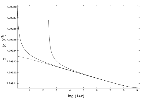
Figure 1: Evolution of $\alpha$ in the background (dashed line) and inside clusters (solid lines) as a function of $\log(1+z)$. Initial conditions were set to match observations of $\alpha$ variation in ref. murphy . Two clusters virialise at different redshifts, one of them in order to have $\alpha_{c}(z_{v}=1)=\alpha_{0}$. Vertical lines represent the moment of turn-around.

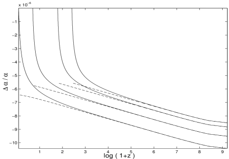
Figure 2: Evolution of $\Delta\alpha/\alpha$ in the background (dashed lines) and inside clusters (solid lines) as a function of $\log(1+z)$. Initial conditions were set to match observations of $\alpha$ variation in ref. murphy . Four clusters that virialised at different redshifts. All clusters were started so as to have $\alpha_{c}(z_{v})=\alpha_{0}$.

If we could measure $\alpha$ inside virialised overdensities and the corresponding value in the background, at the time of their virialisation, then Fig 3 and 4 would give us the evolution of $\alpha_{v}$ or its time shift, $\Delta\alpha_{v}/\alpha_{v},$ as a function of $z_{v}$. Those figures show us that differences in between the background and the overdensities increase as $z_{v}\rightarrow 0$. This is due to the earlier freezing of the value of $\alpha$ at virialisation, and to our assumption that we live in a $\Lambda CDM$ universe. At lower redshifts, specially after $\Lambda$ starts to dominate, variations in $\alpha$ in the background are turned off by the accelerated expansion. However, the value of $\alpha$ in the collapsing cluster will keep growing until virialisation occurs. Numerical simulations give $\Delta\alpha/\alpha(z=2)=-6\times 10^{-6}$ for the background and $\Delta\alpha/\alpha(z_{v}=0.13)=-1.5\times 10^{-7}$ in a cluster. At higher redshifts, $z\gg 1$, both $\alpha_{b}$ and $\alpha_{c}$ evolve in expanding environments: their increase is logarithmic in time before $\Lambda$ starts to dominate, so the difference between them will be much smaller.

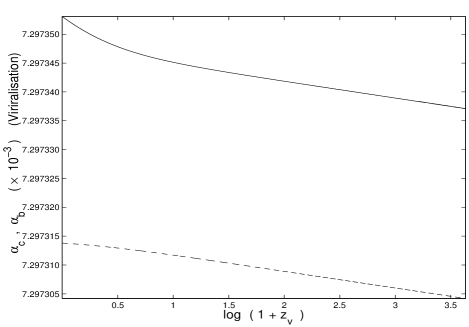
Figure 3: Plot of $\alpha$ as a function of $\log(1+z_{v})$, at virialisation. Clusters (solid line), background (dashed line).

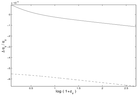
Figure 4: Plot of $\Delta\alpha/\alpha$ as a function of $\log(1+z_{v})$, at virialisation. Clusters (solid line), background (dashed line).

Spatial variations in $\alpha$ can be tracked using a ’spatial’ density contrast, defined by $\delta\alpha/\alpha\equiv[\alpha_{c}-\alpha_{b}]/\alpha_{b}$. A plot of the spatial inhomogeneities in $\alpha$ with respect to the matter density inhomogeneity, $\delta\rho/\rho,$ at virialisation is shown in Fig. 5. Note that $\delta\alpha/\alpha$ grows in proportional to the density contrast of the matter inhomogeneities ($\propto t^{2/3}$ when both are small during dust domination mota2 ). In a $\Lambda CDM$ model, the density contrast, $\Delta_{c}=\rho_{cdm}(z_{v})/\rho_{b}(z_{v})$ increases as the redshift decreases. For high redshifts, the density contrast at virialisation becomes the asymptotically constant in standard ($\Lambda=0$) CDM, $\Delta_{c}\approx 178$ at collapse or $\Delta_{c}\approx 148$ at virialisation. This is another reason why at lower redshifts the difference between $\alpha_{v}$ and $\alpha_{b}$ increases. Trends of variation in $\alpha$ can be then predicted from the value of the matter density contrast of the regions observed. Useful fitting formulas for the dependence of $\alpha$ variation on $\delta\rho/\rho$ and the scale factor $a$ $\equiv(1+z)^{-1}$ are:

$$\delta\alpha/\alpha = (5.56-0.7\sigma^{\frac{1}{2}}+0.078\sigma+0.00352\sigma^{\frac{3}{2}})\times 10^{-6}$$

$$\delta\alpha/\alpha = (5.37+0.373\theta^{\frac{1}{6}}-0.27\theta^{\frac{1}{3}}+0.007\theta^{\frac{1}{2}})\times 10^{-6}$$

$$\Delta\alpha/\alpha = -(2.47-1.81\sigma^{\frac{1}{2}}+0.59\sigma-0.094\sigma^{\frac{3}{2}})\times 10^{-6}$$

where $\theta\equiv\frac{\delta\rho}{\rho}/\Delta_{c_{v}}$, $\sigma\equiv a/a_{v}$. $\Delta_{c_{v}}$ and $a_{v}$ are ’input’ parameters defined when $\alpha(z_{v})=\alpha_{0}$ .

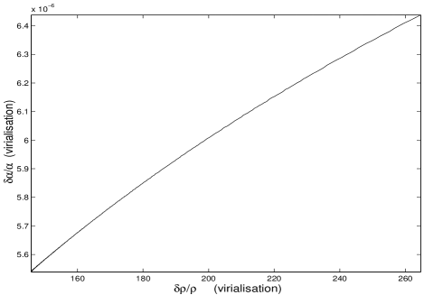
Figure 5: Variation of $\delta\alpha/\alpha$ with $\delta\rho/\rho$ at the cluster virialisation redshift. The evolution of $\alpha$ inside the clusters was normalised to satisfy the latest time-variation observational results, and to have $\alpha_{c}(z_{v})=\alpha_{0}$ for ${z}_{v}{=1.}$

The evolution of $\alpha\equiv\alpha_{b}$ in the background and inside clusters depends mainly on the dominant equation of state of the universe and the sign of the coupling constant $\frac{\zeta}{\omega},$ which is determined by the theory and the dark matter identity. Here, we have assumed that $\omega=1$, so all the dependence is in $\zeta$. As shown in refs. bsm1 , $\alpha_{b}$ will be nearly constant for accelerated expansion and also during radiation-domination far from the initial singularity (where the kinetic term, $\rho_{\psi}$, can dominate). Evolution of $\alpha$ will occur during the dust-dominated epoch, where $\alpha$ increases logarithmically in time for $\zeta<0$. When $\zeta$ is negative, $\alpha$ will be a growing function of time but will fall for $\zeta$ positive bsm1 . Inside clusters $\alpha_{c}$ will have the same dependence on $\zeta$ as it has in the background. The sign of $\zeta$ is determined by the physical character of the dark matter that carries electromagnetic coupling: if it is dominated by magnetic energy then $\zeta<0$, if not then $\zeta>0.$ Our numerical simulations were performed assuming $\zeta=-2\times 10^{-4}$. If we had chosen $\zeta$ to be positive we would find that $\alpha_{b}$ would decrease as steeply as $z\rightarrow 0$. We choose the sign of $\zeta$ to be negative so $\alpha$ is a slowly growing function in time during dust domination. This is done in order to match the latest observations which suggest that $\alpha$ had a smaller value in the past murphy . However, we know that on small enough scales the dark matter will become dominated by a baryonic contribution for which $\zeta>0.$ This will create distinctive behaviour and will be investigated separately. Generally, past studies of spatially homogeneous cosmologies have effectively matched the value of $\alpha_{b}$ with the terrestrial value of $\alpha$ measured today. However, it is clear that the value of the fine structure constant on Earth, and most probably in our local cluster, will differ from that in the background universe. This feature has been ignored when comparing observations of $\alpha$ variations from quasar absorption spectra murphy with local bounds derived by direct measurement prestage or from Oklo oklo and long-lived $\beta$-decayers beta . A similar unwarranted assumption is generally made when using solar system tests of general relativity to bound possible time variations in $G$ in Brans-Dicke theory varyg : there is no reason why $\dot{G}/G$ should be the same in the solar system and on cosmological scales. Since any varying-constant’s model require the existence of a scalar field coupled to the matter fields, our considerations apply to all other theories besides BSBM and to variations of other ’constants’ other . Note that this feature is much less important when using early universe constraints like the CMB or BBN cmbbbn , since small perturbations in $\alpha$ will decay or become constant in the radiation era mota2 .

In summary, using the BSBM theory we have shown that spatial variations in $\alpha$ will inevitably occur because of the development of large density inhomogeneities in the universe. This was first shown in the linear regime, when perturbations are small mota2 , and then $\frac{\delta\alpha}{\alpha}$ tracks $\frac{\delta\rho_{m}}{\rho_{m}}$ during the dust-dominated era on scales smaller than the Hubble radius. We have used the spherical collapse model to study the space-time variations in $\alpha$ in the non-linear regime. Strong differences arise between the value of $\alpha$ inside a cluster and its value in the background and also between clusters. Variations in $\alpha$ depend on the matter density contrast of the cluster region and the redshift at which it virialised. If the overdense regions are still contracting and have not yet virialised, then the value of $\alpha$ within them will continue to change. Variations in $\alpha$ will cease when the cluster virialises so long as it does so at moderate redshift. This leads to larger values of $\alpha$ in the overdense regions than in the cosmological background and means that time variations in $\alpha$ will turn off in virialised overdensities even though they continue in the background universe. The fact that local $\alpha$ values ’freeze in’ at virialisation, means we would observe no time or spatial variations in $\alpha$ on Earth, or elsewhere in our Galaxy, even though time-variations in $\alpha$ might still be occurring on extragalactic scales. For a cluster, the value of $\alpha$ today will be the value of $\alpha$ at the virialisation time of the cluster. We should observe significant differences in $\alpha$ only when comparing clusters which virialised at quite different redshifts. Differences will arise within the same bound system only if it has not reached viral equilibrium. Hence, variations in $\alpha$ using geochemical methods could easily give a value that is $100$ times smaller than is inferred from quasar spectra. We conclude that the consideration of the evolution of inhomogeneities, notably the one inside which we live, is essential if we are to make meaningful comparisons of different pieces of astronomical and terrestrial evidence for the constancy of $\alpha$.

References

- (1) M.T.Murphy et al., MNRAS, 327, 1208 (2001). J.K.Webb et al., Phys. Rev. Lett. 87, 091301 (2001). J.K.Webb et al., Phys. Rev. Lett. 82, 884 (1999). M.T.Murphy et al., Astrophys. Space Sci. 283, 577 (2003).
- (2) H.B.Sandvik et al., Phys. Rev. Lett. 88, 031302 (2002); P.Brax et. al, Astrophys. Space Sci. 283, 627 (2003); J.D.Bekenstein, Phys. Rev. D 25, 1527 (1982); Phys. Rev. D 66, 123514 (2002) and astro-ph/0301566. D.Youm, Mod. Phys. Lett. A 17, 175 (2002).
- (3) P.Langacker et al., Phys.Lett. B528, 121(2002); T.Dent et al., Nucl. Phys. B 653, 256(2003); X.Calmet et al., Eur. Phys. J. C 24(2002) 639; H.Fritzsch, hep-ph/0212186.
- (4) J.D.Barrow et al., Class. Quant. Grav. 19, 6197 (2002). J.D.Barrow et al., Phys. Rev. D 65, 063504 (2002); Phys. Rev. D 65, 123501 (2002) and Phys. Rev. D 66, 043515 (2002).
- (5) J.D.Barrow et al., Class. Quant. Grav. 20, 2045 (2003)
- (6) J.D.Barrow et al., MNRAS 322, 585 (2001). J.D.Barrow et al., Int. J. Mod. Phys. D 11 (2002) 1615.
- (7) J.D.Prestage et al., Phys. Rev. Lett. 74, 18 (1995). Y.Sortais et al, Physica Scripta T95, 50 (2001)
- (8) Y.Fujii et al., Nucl. Phys. B 573, 377 (2000). T.Damour et al., Nucl. Phys. B 480, 37 (1996).
- (9) K.A.Olive et al., Phys. Rev. D 66, 045022 (2002).
- (10) T. Padmanabhan, ’Structure formation in the universe’, CUP, Cambridge, 1995; J. Peacock ’Cosmological Physics’, CUP. Cambridge 1999.
- (11) P.D.Scharre et al., Phys. Rev. D 65, 042002 (2002).
- (12) A.Ivanchik et al., Astrophys. Space Sci. 283, 583 (2003). J.P. Uzan, Rev. Mod. Phys. 75, 1403 (2003).
- (13) C.J.A.P.Martins et al., astro-ph/0302295. P.P.Avelino et al., Phys. Rev. D64 (2001) 103505.