Constraining Dark Energy Evolution with Gravitational Lensing by Large Scale Structures

Abstract

We study the sensitivity of weak lensing by large scale structures to the evolution of dark energy. We explore a 2-parameters model of dark energy evolution, inspired by tracking quintessence models. To this end, we compute the likelihood of a few representative models with varying and non varying equation of states. Based on an earlier work, we show that the evolution of dark energy has a much stronger impact on the non-linear structure growth than on the angular diameter distance, which makes large scale structure measurements a very efficient probe of this evolution. For the different models, we investigate the dark energy parameters degeneracies with the mass power spectrum shape $\Gamma$, normalisation $\sigma_{8}$, and with the matter mean density $\Omega_{M}$. This result is a strong motivation for performing large scale structure simulations beyond the simple constant dark energy models, in order to calibrate the non-linear regime accurately. Prospective for the Canada France Hawaii Telescope Legacy Survey (CFHTLS) and Super-Novae Acceleration Probe (SNAP) are given. These results complement nicely the cosmic microwave background and Super-Novae constraints. Weak lensing is shown to be more sensitive to a variation of the equation of state, whereas CMB and SNIa give information on its constant part.

Dark energy is a generic way to describe the acceleration of the universe. Within this framework, the acceleration of the expansion measured by the type Ia Super-Novae surveys Perlmutter et al. (1999); Riess et al. (2001) is explained by the contribution of a new component. In a FRLW metric, this component is described by its equation of state. In this paradigm, the cosmological constant is one possible model, among others, of dark energy.

The question of the properties of this dark energy remains open. Different observations have been proposed to evaluate them. Measurement of the distances to Super-Novae Astier (2001); Maor et al. (2001); Goliath et al. (2001) or of the size of structures on the CMB Brax et al. (2000); Doran and Lilley (2002) provide informations on how the dark energy modifies the relation between cosmological distances and redshifts. The evolution of large scale structures also probe the properties of dark energy. This kind of tests can be built using cluster abundances Haiman et al. (2001); Weller et al. (2002); Hu (2003), Ly-$\alpha$ forest Seljak et al. (2002), strong Bartelmann et al. (2002a); Sereno (2002) and weak lensingBenabed and Bernardeau (2001); Huterer (2002); Hu (2002); Bartelmann et al. (2002b); Weinberg and Kamionkowski (2003)…

In this article, we will investigate the weak lensing constraints in the case of a varying equation of state. This case has been first investigated qualitatively by Benabed and Bernardeau Benabed and Bernardeau (2001) (hereafter BB01). We will expand their results and propose the first quantitative analysis of the efficiency of the shear two points function to probe varying equation of state dark energy models. The constraints on the dark energy using the linear regime alone are not particularly strong, even using the tomography technique Hu (2002). Here, we take into account the non-linear regime of gravitational collapse, which is known to convey much of the dark energy sensitivity Benabed and Bernardeau (2001), and we study the degeneracy of the dark energy parameters with the matter density $\Omega_{M}$, the mass power spectrum shape $\Gamma$ and normalisation $\sigma_{8}$.

As said above, large scale structures are sensitive to the expansion rate of the universe, which makes the structure growth sensitive to the dark energy content of the Universe Benabed and Bernardeau (2001). This sensitivity is due to the fact that when the dark energy starts to dominate the energy budget of the Universe, the efficiency of the gravitational collapse is reduced. Hence, the density fluctuations growth changes when the dark energy differs from a simple cosmological constant. For models within the current SNIa constraints, it corresponds to a slower growth in the linear regime. The stronger the variation in the evolution of dark energy, the earlier this effect occurs and the more suppressed will be the structure growth. Keeping the amplitude of density fluctuations fixed today, this translates into an earlier entrance of the fluctuations in the non-linear regime, leading to more concentrated dark matter halosKlypin et al. (2003); Linder and Jenkins (2003), and therefore stronger lenses Sereno (2002). As shown in BB01, the shear two points function is sensitive to these two effects. It provides an unbiased measure of the projected density power spectrum in both the linear and non-linear regimes, which is a direct test of the evolution of large scale structures, and through it, a measure of the properties of dark energy. In particular, the scale at which the transition between the two regimes occurs is tested. This feature is the key to constraint the properties of dark energy.

In the following, we first review the computation of the shear two points function with a dark energy component. Then, we propose a simple two parameters model that encompass the major features of a generic class of dark energy, namely the tracking quintessence models. Next, we address the question of the efficiency of future lensing surveys to determine the dark energy properties.

I Theory

We establish in this section the theoretical basis of the result presented in section II. We show here how to compute the non-linear cosmic shear power spectrum with a non-trivial dark energy, and how it is evaluated from the data. We discuss the sensitivity of this quantity to the evolution of an hypothetical dark energy component. We then propose a dark energy equation of state parameterization suitable for a class of dark energy models.

I.1 Cosmology

Lets assume that the dark energy component is minimally coupled to the universe, which means that it interacts with the rest of the Universe via gravity only. The expansion of the universe is completely described by the Friedmann equations

$$\left(\frac{\dot{a}}{a}\right)^{2} = \frac{8\pi}{3M_{\textrm{Planck}}}\sum\rho_{\textrm{X}}$$ (1)

$$\frac{\ddot{a}}{a} = -\frac{4\pi}{3M_{\textrm{Planck}}}\sum\left(\rho_{\textrm{X}}+3p_{\textrm{X}}\right).$$ (2)

and the knowledge of an equation of state for each component

$$P_{\textrm{X}}=w_{\textrm{X}}\,\rho_{\textrm{X}}.$$ (3)

The radiation, matter and curvature equation of state are fixed. The only unknown quantity here, is the equation of state parameter of the dark energy, $w_{Q}$. It usually varies between $+1$ and $-1$. The case $w_{Q}=-1$ corresponds to a cosmological constant.

It has been proposed recently that $w_{Q}$ can also take values lower than $-1$ Carroll et al. (2003). This is only possible if the dark energy has a negative kinetic energy. Such unusual behavior have only been found in very specific modelsOnemli and Woodard (2002), and it is not yet clear if it has any physical meaning. Therefore, we keep the conservative prior $w_{Q}\geq-1$.

We also assume that the dark energy does not fluctuate and thus is not coupled to the fluctuations of the matter density. This is of course not true in general: it is expected that dark energy fluctuates from one Hubble volume to the next, which is expected to leave an imprint on the metric fluctuations when the universe expands. However, it has been showed that these fluctuations are quickly damped by the evolution. Moreover, it is expected that they are negligible on scales smaller than the horizon at recombination Ferreira and Joyce (1998); Malquarti and Liddle (2002); Brax et al. (2000). In the following, we only consider such scales and can thus safely ignore these fluctuations.

With these assumptions, the impact of dark energy on the evolution of the large structures is completely described by the equation of state Benabed and Bernardeau (2001).

I.2 Shear measurements on distant galaxies

The deviation of light by the gravitational potential wells distorts the image of the distant galaxies. This shear effect can be used to probe the projected mass distribution along the line of-sight (see and references Bartelmann, Matthias and Schneider, Peter (1999) therein), from a measurement of the shape of the lensed galaxies. The lensing effect produced by the large scale structures is weak, but has already been measured Van Waerbeke and Mellier (2003).

The gravitational lensing effect depends on the second order derivatives of the gravitational potential projected along the line-of-sight. The convergence $\kappa$ and the shear $\bf\gamma$ describe the distortion of the image of the distant images (located at some redshift $z_{s}$), by the inhomogeneous matter distribution along the line-of-sight. At linear order, convergence and shear field are related

$$\Delta\kappa=\left(\partial_{1}^{2}-\partial_{2}^{2}\right)\gamma_{1}+2\partial_{1}\partial_{2}\gamma_{2}$$ (4)

At the same order, the convergence in the direction $\bf\theta$, which describes the isotropic change of the image at position $\chi_{s}$, is given by:

$$\kappa(\hbox{$\bf\theta$}) = {\frac{3}{2}}{\frac{H_{0}}{c}}^{2}\Omega_{0}$$

$$\int_{0}^{\chi_{S}}{\textrm{d}}\chi\;{\frac{\mathcal{{D}}(\chi_{s}-\chi)\,\mathcal{{D}}(\chi)}{\mathcal{{D}}(\chi_{s})}}{\frac{\delta\left(\mathcal{{D}}(\chi)\hbox{$\bf\theta$},\chi\right)}{a(\chi)}},$$

where $\chi_{s}(z_{s})$ is the source radial distance located at redshift $z_{s}$, and $a=1/(1+z)$ is the scale factor. The radial distance at redshift $z$ is given by

$$\chi(z)=\int_{0}^{z}{\textrm{d}}z^{\prime}{\frac{c}{H}}.$$ (6)

The angular diameter distance $\mathcal{{D}}$ is defined by

$$\mathcal{{D}}(\chi)=\left\{\begin{array}[]{ll}\sin(\sqrt{K}\chi)/\sqrt{K},&K>1\\ \chi,&K=1\\ \sinh(\sqrt{K}\chi)/\sqrt{K},&K<1\end{array}\right.$$ (7)

where $K$ is the curvature. As a consequence, the weak lensing effect is a direct and unbiased measurement of the projected density contrast.

We focus on the convergence power spectrum $P_{\kappa}(\ell)$. It can be shown Bernardeau et al. (1997); Jain and Seljak (1997) that it is directly related to the 3-dimensional mass power spectrum $P_{3D}$ via:

$$P_{\kappa}(\ell) = {\frac{9}{4}}\left(\frac{H_{0}}{c}\right)^{4}\Omega_{0}^{2}$$

$$\int_{0}^{\chi_{S}}{\textrm{d}}\chi^{\prime}\;{\frac{g^{2}(\chi^{\prime})}{\mathcal{D}^{2}(\chi^{\prime})a^{2}(\chi^{\prime})}}P_{3D}\left({\frac{\ell}{\mathcal{D}(\chi^{\prime})}},\chi^{\prime}\right),$$

where the $g(\chi)$ function describe the lensing efficiency,

$$g(\chi)=\frac{\mathcal{{D}}(\chi_{s}-\chi)\,\mathcal{{D}}(\chi)}{\mathcal{{D}}(\chi_{s})}.$$ (9)

When the lensed galaxies are distributed in redshift, the observed signal is given by Eq.9 integrated among the source redshift distribution $p_{s}(\chi)$. In that case, the $g(\chi)$ function becomes:

$$g(\chi)=\mathcal{D}(\chi)\int_{\chi}^{\chi_{s}}{\textrm{d}}\chi^{\prime}\;p_{s}(\chi^{\prime})\,{\frac{\mathcal{D}(\chi_{s}-\chi^{\prime})}{\mathcal{D}(\chi_{s})}}.$$ (10)

The source redshift distribution $p_{s}(z)$ is normalised, and usually parametrised as

$$p_{s}(z)=\Gamma^{-1}\left({\frac{1+\alpha}{\beta}}\right){\frac{\beta}{z_{s}}}\left({\frac{z}{z_{s}}}\right)^{\alpha}\leavevmode\nobreak\ \exp\left[-\left({\frac{z}{z_{s}}}\right)^{\beta}\right].$$ (11)

The free parameters $\alpha$, $\beta$ and $z_{s}$ are adjusted to accommodate different survey properties.

The ellipticity of the galaxies is an unbiased measure of the shear, from which we derive the statistical properties of the convergence field (see a review of the observational results in Van Waerbeke and Mellier (2003)). In practice, the statistic of interest is the aperture mass variance as function of scale, $\langle M_{\textrm{ap}}^{2}(\theta)\rangle$ Schneider et al. (1998), also called the $M_{\textrm{ap}}$ statistic. It links the variance of the convergence field (which is the field of physical interest, because proportional to the projected mass density) and the shear (which is the observable quantity). Its main feature is to provide a natural separation between the cosmological signal (which is curl-free) and the systematics (contributing to the curl mode). It has already been measured on several galaxy surveys Van Waerbeke and Mellier (2003). The $M_{\textrm{ap}}$ statistic at a scale $\theta_{c}$ is defined as the convergence smoothed with a compensated filter $U(\hbox{$\bf\theta$})$. Using Eq. (4), it is also given by a properly smoothed shear component $\gamma_{t}$:

$$M_{\textrm{ap}} = \int_{0}^{\theta_{c}}{\textrm{d}}^{2}\theta\;U(\theta)\;\kappa(\hbox{$\bf\theta$})$$ (12)

$$= \int_{0}^{\theta_{c}}{\textrm{d}}^{2}\theta\;Q(\theta)\;\gamma_{t}(\hbox{$\bf\theta$}),$$ (13)

with $\int_{0}^{\theta_{c}}{\textrm{d}}\theta\;\theta\;U(\theta)=0$, and where

$$Q(\theta)={\frac{2}{\theta_{c}^{2}}}\int_{0}^{\theta_{c}}{\textrm{d}}\theta^{\prime}\;\theta^{\prime}\,U(\theta^{\prime})-U(\theta).$$ (14)

The tangential shear $\gamma_{t}$ at a location $\hbox{$\bf\theta$}=(\theta\cos\varphi,\theta\sin\varphi)$ is defined by

$$\gamma_{\textrm{t}}(\hbox{$\bf\theta$})\equiv-\Re\left(\gamma(\hbox{$\bf\theta$})\,{\textrm{e}}^{-2{\textrm{i}}\varphi}\right).$$ (15)

The choice of $U(\theta)$ is arbitrary provided it has a zero mean. In the following, we will use Van Waerbeke and Mellier (2003)

$$U(\theta)\equiv{\frac{9}{\pi\theta_{c}^{2}}}\left(1-\left({\frac{\theta}{\theta_{c}}}\right)^{2}\right)\left({\frac{1}{3}}-\left({\frac{\theta}{\theta_{c}}}\right)^{2}\right).$$ (16)

For this particular choice, the variance of the convergence is expressed in term of the shear power spectrum as

$$\langle M_{\textrm{ap}}^{2}\rangle={\frac{288}{\pi}}\int{\textrm{d}}\ell\;\ell\;P_{\kappa}(\ell)\left[{\frac{J_{4}(\ell\theta_{c})}{\ell^{2}\theta_{c}^{2}}}\right]^{2}.$$ (17)

The variance of the aperture mass is therefore a broad-band estimate of the convergence power spectrum given in Eq.(9), which can directly be estimated from the galaxy shapes. This is the quantity which will be used to study the evolution of dark energy in section II. In order to make predictions on cosmic shear observable, one only needs to compute the convergence power spectrum in dark energy. As shown in Eq. (I.2), it only depends on the cosmology through the relation between angular distances and redshifts, and through the power spectrum of the matter density fluctuations. The source distribution $p(z)$ can be determined from the data and does not depend on the cosmology.

A complete discussion on the computations of the weak lensing power spectrum with a cosmology with a non-trivial dark energy has been done in BB01. We only reproduce here the conclusions of this work.

I.3 Cosmological distances

The relation between the cosmological distances and redshift is given by eq. (6). The dark energy component only leaves an imprint on $\chi(z)$ by modifying the acceleration of the universe obtained by solving Eq. (1-2).

The modification of the relation distance / redshift affects mildly the convergence power spectrum. It can be summarized into two simple effects : a normalization change and a scale shift (similar to the modification of the position of peaks in CMB).

The lensing efficiency function (Eq. 9-10) acts as a selection window. It is maximum for lenses located roughly at mid-distance between the observer and the source galaxies. This selection effect can be approximated by replacing the $g(\chi)^{2}$ term in in Eq. (I.2) by a Dirac function

$$g^{2}(\chi)\sim g^{2}(\chi_{\textrm{mid}})\delta(\chi-\chi_{\textrm{mid}}).$$ (18)

In this approximation, the normalization change advertised earlier is driven by the change in the position of the maximum of the selection function.

The scale shift is also easily understood with this approximation. This shift comes from the $P_{3D}(\frac{\ell}{\mathcal{D}(\chi)})$ term in Eq. (I.2). The modification of the maximum of the efficiency window selects a different depth for projection.

In the following, we will show that the matter power spectrum can be split into two evolution regimes. At large scale, the linear regime is well described by a power law. The effect of dark energy can be completely re-absorbed into a change in normalization. At small scales however, in the non-linear regime, the power law approximation is no longer a good description of the power spectrum. Like the modification of the peaks in the CMB power spectrum, the scale under which is seen the transition from linear to non-linear regime will be slightly shifted by the above effect.

I.4 Power spectrum of matter

From a practical point of view, there is no need to compute the whole power spectrum of the density fluctuation. Only a narrow range of scale, from a few arc-second (galaxy scale) to a few hundreds of arc-minutes across the sky is enough. Large scales ($>\leavevmode\nobreak\ 5$ degrees) are difficult to access observationally anyway; the weak lensing correlation amplitude is small, where the residual systematics might be a problem, and the surveys capable of such measurement are not yet planned. At scales smaller than a few arc-seconds, the number of lensed galaxies drops, and the noise blows up.

At redshift one, a few degrees corresponds to a few hundreds of Mpc, which is far below the horizon size at recombination. As stated in section I.1 we can safely assume that for the scales of interest, a classic CDM power spectrum is a good approximation of the power spectrum of the matter density fluctuation. Moreover, for these scales, the power spectrum behaves essentially as a power law. The remarks made above on the cosmological distances holds, and the effect of the modification of the equation of state of dark energy on the cosmological distances translate, for this range of scales, in a simple normalization shift.

We have yet to investigate the evolution of the power spectrum from recombination until now. The growth of structures is modified by the presence of a dynamic dark energy component. At the linear order, it is given by the well known equationPeebles (1993)

$$\ddot{D}_{+}(t)+2H\dot{D}_{+}(t)-\frac{3}{2}H^{2}\,\Omega_{0}(t)\,D_{+}(t)=0.$$ (19)

In this equation, the matter acts as a source term that increases the depth of the potential well and tends to increase the density contrast. On the opposite, the expansion of the universe acts, via the second term, as a friction effect and reduces the efficiency of gravitation to increase the density contrast. This term carries all the effect of dark energy on the growth of structures.

At high redshift, the dark energy is completely dominated by the radiation or the matter density. During the radiation era, the growing mode of equation Eq. (19) can be obtained analytically

$$D_{+}\propto a^{\frac{3}{2}}.$$ (20)

During matter domination, the solution is also well known

$$D_{+}\propto a.$$ (21)

These remarks allow us to integrate Eq. (19) in our model; we do not know any other initial condition that would allow us to perform the integration and be sure to keep the growing solution.

It is worth noting here that there is no other way to compute the growth of structureBenabed and Bernardeau (2001); Linder and Jenkins (2003). The well known integral solution of Eq. (19) is valid when the universe only contains matter, radiation curvature and a cosmological constant. It is also easy to convince oneself that there is no solution to Eq. (19) that can be integrated from today toward the past. Equation (19) generically admits a growing and a non-growing solution. Only the first one is of cosmological interest, and there is no way to build this solution when integrating from the final point of the evolution.

During the expansion, the growth follows the radiation, and then the matter solution. When dark energy gets closer to the energy density of matter, the friction term grows compared to the source one. The efficiency of gravitational collapse to build up the density perturbation decreases and the growth of structures is damped. For the set of models where the dark energy happens to dominate earlier, this reduction of the growth rate is experienced at a higher redshift. The exact starting point of this damping depends on the evolution properties of the dark energy model. Models with $w_{Q}>-1$ experience this effect earlier than for $w_{Q}=-1$. For a constant equation of state, the energy density of the dark energy goes as

$$\Omega_{Q}\propto a^{-3(1+w_{Q})}.$$ (22)

As said above, the $w_{Q}=-1$ model is the cosmological constant case. When $w_{Q}>-1$, $\Omega_{Q}$ grows as the scale factor $a$ goes to unity. In this case, the dark energy contribution to the expansion is significant at a higher redshift than when $w_{Q}=-1$. This is even more important for varying $w_{Q}$, as shown figure 1. The modelling of the dark energy used in this figure will be described later.

Figure 1: The energy density of dark energy normalized to the critical density as a function of redshift. Thick plain line is the classic $\Lambda$ model. The thick long dashed line and thin dot dashed line are resp. a $w_{Q}=-0.8$ and $w_{Q}=-0.6$ models. The short dashed and dotted line are resp. $w_{0}=-0.8,\>w_{1}=0.2$ and $w_{0}=-0.8,\>w_{1}=0.3$ models (complete description of the parameterization can be found sec. I.5). The sooner the dark energy gets close to one, the sooner it will affect the expansion and the growth of structure. As expected, models with a equation of state different from $w_{Q}=-1$ contribute significantly to the acceleration sooner. Models with a varying equation of state contribute yet sooner. A constant $w_{Q}=-0.6$ model interpolates between the two $w_{1}\neq 0$ ones.

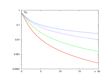
Figure 2 shows the result of a numerical integration of eq. (19) for different models. The damping of the growth appears earlier in the varying equation of state models, compared to the constant equation of state.

Figure 2: linear growth for different models. Models are the same than fig. 1.The growth are normalized to the recombination era. The modification of the equation of state induce a precocious acceleration that decrease the efficiency of gravitational collapse at higher redshift than in the $w_{Q}=-1$ case. A variation in the equation of state ($w_{1}\neq 0$) amplify this effect. As expected from fig. 1 a constant equation of state model can partly mimic a varying equation of state: if one knows the CMB normalization and today normalization of the fluctuation of structures, one cannot distinguish between a $w_{Q}=-0.6$ and a $w_{0}=-0.8,\>w_{1}=0.3$ models.

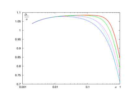
For a fixed redshift, the modification of the growth of structure at linear order will be degenerated with the normalization of the power spectrum. Of course, following the linear power spectrum along the line of sight allows to break this degeneracy. Unfortunately, the measured shear power spectrum is only a projection of the mass power spectrum along the line of sight. We showed in previous section that this projection acts like a selection effect on a single redshift plane. Therefore, the integrated growth effect will be, in the linear part of the lensing power spectrum, indistinguishable from a normalization shift.

At small scales, the evolution of the density contrast changes dramatically. Virialized objects are formed and evolve in a different regime than the simple one described by the linear approximation. BB01 showed that this regime can potentially solve part of the degeneracy described above. The weak lensing measurement on galaxies allows access to the bigger scales of this non-linear regime.

The perturbation approach cannot describe this regime as the density contrast is very big at the scale of virialized objects. A complete computation of this regime cannot be done analytically. One has to rely on hypotheses on the properties of this regime to be able to describe it. Several “classic” description of this regime has been proposed (among others see Hamilton et al. (1991); Peacock and Dodds (1996); Cooray and Sheth (2002)). We will follow here the choices made in BB01. We assume that the Stable Clustering Ansatz provide a valid description of the smaller scales of the non-linear regime. It states that virialized objects are stable, that is to say that their physical size does not vary with the expansion of the universe. Hence, at the scale of these objects, the density contrast has to grow to match exactly the expansion. Instead of a growth of order $a$ or smaller, the density contrast evolves as $a^{3/2}$.

One should note that the scales described by the Ansatz are below the shear measurement scales. The transition between the linear and non-linear regimes is described by a mapping between the two regimes Hamilton et al. (1991). This mapping is calibrated using a fit to n-body simulations, as described in Peacock & Dodds Peacock and Dodds (1996). At large scale, the mapping keeps unchanged the linear regime, and at small scales, it must go as $(a^{2}/g^{2}P)^{3/2}$. Although this type of mapping has been widely tested for many different cosmologies, it has never been tested for dark energy models. However, given the robustness of the mapping for very different cosmologies, we assumed it remains valid for the class of models studied here.

This is a very strong assumption. It can partly be justified by the fact that it is unlikely that a smoothed dark energy component with no coupling can affect the small scale behavior of the matter. Its influence should only appear as a change in the expansion and thus, as we have shown above, as a modification of the linear growth of structures. The strength of this argument argument is enhanced by a recent result from another description of the non-linear regime usually called the halo model. This approach describes the virialized object as dark matter halos of known profile and abundance depending on the cosmological parameters Cooray and Sheth (2002). The results and concepts behind this approach have been successfully tested in the context of dark energy Klypin et al. (2003); Linder and Jenkins (2003). In particular the differences observed between halos in $\Lambda$ cosmologies and in cosmology with non trivial dark energy can be explained by an earlier entrance into the non-linear regime. The observed discrepancies are, as expected, all explained by the modification of the linear growth of structures Benabed and Bernardeau (2001); Bartelmann et al. (2002b).

As we just emphasized above, the effect of a non trivial dark energy on the non-linear regime are all encoded in the linear growth. As the structures grow slowly, they reach the non-linear regime earlier (for the same final normalization). Thus, changing their growth at a higher redshift they undergo a longer non-linear evolution. This translates, in the context of Stable Clustering Ansatz into a higher asymptote of the power spectrum at large wave numbers Benabed and Bernardeau (2001), and in the halo approach, into a halo profile with more substructure and more mass in the center Klypin et al. (2003). Note that the case described here is very similar to a comparison between an open and a flat model.

This will show up in the weak lensing power spectrum in two ways. First, the earlier entrance in the non-linear regime, once projected, gives a transition between the linear and non linear regime at smaller $\ell$. Second, the amplitude of the power spectrum at small scale is expected to be higher. BB01 proposed estimations of these two effects. In particular, due to the different evolution in the non-linear regime, the modification of the asymptote height is expected to go as the third power of the normalization modification in the linear regime.

Probing the small scales of the shear power spectrum will reduce the degeneracy between the determination of dark energy properties and the normalization of the matter density fluctuation. The extend to which this can be done is the main subject of sec. II.

Before going to next section, we would like to emphasize the fact that any modification in the nature of dark matter will be degenerated (at the level of the growth of structures of course) with the effect of dark energy. In particular, inclusion of hot dark matter will also modify the rate of growth. It is expected that this modification should decrease the amount of small scale structure, thus suppressing the effect of dark energy. We are then likely to underestimate the effect of dark energy in those models.

I.5 Dark Energy Model

The evolution of $w_{Q}$ is a priori free. It has to be fixed by a proper model of dark energy. Several models have been studied. The simplest being the minimal quintessence model, where $w_{Q}$ is constant. Another very interesting class of models are the so-called tracking potential models.

These models have been extensively described Steinhardt et al. (1999). Their interest lie in the fact that their equation of state parameter is constant during most of the universe evolution. The constant equation of state is an attractor solution for $w_{Q}$ when the expansion of the universe is dominated by another component (like the radiation or the matter). Of course, when the dark energy reaches the order of magnitude of the other energy densities, it leaves its attractor evolution. This attractor ensures that the initial conditions of dark energy does not have to be finely tuned. Whatever is the starting value of the dark energy, it has to reach the attractor and will always exit the domination of matter at the same point, which in turn depends of the exact model.

This explains the interest these models have met among the high energy physics community. In particular, it has been shown that some tracking potential models can be built within particle physics models. For example, P. Brax and J. Martin Brax and Martin (2000) proposed a version of the Ratra-Peebles model Peebles and Ratra (1988) that can be embedded in super-gravity models.

Minimal and tracking models are not the only dark energy models available. The problem however is that it does not exist any common framework to describe the different dark energy models that allows a direct comparison between them as we plan to do here, in the context of weak lensing. We attempt here to provide a suitable parameterization that will allow to constrain the dark energy properties using shear measurements. This is a simplification of the problem: we only have to model the evolution of dark energy that can leave an imprint on the weak lensing power spectrum. As a consequence, we only have to consider its impact on the growth of structure and on the relation distance-redshift.

We choose to parameterize the evolution of dark energy in term of its equation of state. This choice is the most prevalent one. This is by no mean the only possible parameterization Alam et al. (2003). As stated in section I.1, the knowledge of the EOS of dark energy is sufficient to solve Eq. (1-2) and to compute $\chi(z)$ and $D_{+}$.

If we do not make any further assumptions, $w_{Q}$ can freely vary between $-1$ and $1$. The easiest solution is to assume that $w_{Q}$ can be written as a power series of the redshift

$$w_{Q}=\sum w_{i}\,z^{i}.$$ (23)

This is the way most SNIa data are analyzed. More precisely, using the fact that the data collected relates directly to the integral of the expansion factor up to a redshift of order one, it is enough to only investigate this equation of state in a perturbative development

$$w_{Q}=w_{0}+w_{1}z\dots$$ (24)

The possible determination of the two first orders of this development Astier (2001); Goliath et al. (2001); Maor et al. (2001) as been studied.

This approach is not valid in our case. As noted above, one can only compute the growth of structure from recombination. A perturbative development as Eq. (24) is of course not suitable for our purposes; it leads to arbitrarily growing equation of state, which is not physical! The full power series is also useless. As explained above, it is in the transition between linear and non-linear scales that one can expect to gain some information on the dark energy. As shown figure 1 and 2, one can expect some level of degeneracy even between a given varying and a non varying EOS models. Accordingly, it is very important here that we greatly reduce the parameter space allowed to $w_{Q}$.

Since we obviously cannot explore completely the equation of state space if we want to restrict ourselves to a small number of parameters, we have to make some assumptions on the behavior of the dark energy equation of state. There are already too many different models of dark energy, and it is impossible to describe them with just one simple parameterization. Attempts have been made to generically describe dark energy with a simpler parameterization than the naive power series. They however produce results with yet to many parameters Corasaniti and Copeland (2002) for our purpose. Another possible approach would be a principal component analysis designed for shear power spectrum inspired from ideas proposed in Huterer and Starkman (2002).

Here, to reduce the complexity, we add a physical assumption. We will only be interested in models who exhibit a behavior similar to the one of the tracking potential models. This is a very strong assumption. If the choice of model is hard to justify, we will however give here a few arguments in favor of the tracking potential behavior.

The behavior of the dark energy equation of state at large redshift is in fact quite irrelevant for us. Indeed, tracking models assures that the equation of state of the dark energy is constant as long as it is dominated by the other components Steinhardt et al. (1999). When dark energy is dominated its variation have little or no impact on the expansion of the universe. The growth of structure is not greatly modified by variation of $w_{Q}$ when the dark energy component does not contribute significantly to the expansion. Accordingly, assuming a constant or varying equation of state during domination of matter or radiation is not relevant to our problem. Of course if one assumes that dark energy can be dominant at high redshift, this discussion is not valid. However, an such a dark energy model would leave a huge imprint on the CMB and would be most probably already ruled out by observations.

Figure 3: Comparison between an explicit SUGRA model and its parameterization. The equations of state are presented on the top panel, whereas the energy density, normalized to the critical density are on the bottom. Plain line is the SUGRA $\alpha=6$ model, long dashed is the logtan parameterization, short dashed, the log parameterization (see Eq. (25) and (29)). The parameter $w_{0}=-0.84$, $w_{1}=0.32$ are measured on the SUGRA model. The log parameterization quickly fails to fit the equation of state above $z\sim 1$. It keeps a relatively good agreement on the dark energy density the to a higher redshift. It is not unexpected as the dominant contribution to $H^{2}$ is already the matter energy density. Thus slight variation on the equation of state of the dark energy are softened on $\Omega_{Q}$. The discrepancy, however build up very quickly to a factor 2 around $z\sim 8$. While not being in perfect agreement with the SUGRA model, the logtan parameterization does a better job at following $\Omega_{Q}$.

At low redshift, when dark energy reaches the order of magnitude of the energy density of matter, it will start to contribute to the expansion, and induce a new period of acceleration. Variations of $w_{Q}$ then leave a potentially strong imprint on the shear power spectrum, through modifications of the cosmological distances and structure growth. This is where our assumption on the shape of the model is important. Other models of the dark energy can have very different behavior. Our choice to only consider tracking like models theoretically reduce the reach of our conclusion, at least in its details.

It has been shown Efstathiou (1999) that the equation of state of tracking models can be fitted at low redshift by a log function

$$w_{Q}\sim w_{0}+w_{1}\log(1+z).$$ (25)

This behavior is roughly valid up to redshift $z\sim 1$ at least for SUGRA and Ratra-Peebles potentials. Note that this equation of state parameter admits Eq. (24) as its Taylor expansion at small $z$.

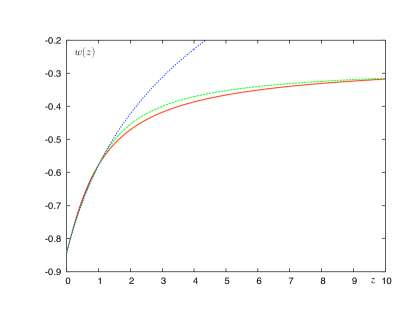
The parameterization given in Eq.(25) fails quickly above $z\sim 1$ (see figure 3 ). It has to be modified to account for the evolution of the equation of state for $z>1$. We propose to use an arctangent which has the property to quickly reach a constant value. We will then use

$$w_{Q} =$$ (29)

$$\left\{\begin{array}[]{l}w_{0}+w_{1}\log(1+z),\>\textrm{if }z\leq 1\\ w_{0}+w_{1}\left[\log(2)-\arctan(1)+\arctan(z)\right],\>\textrm{if }z>1\end{array}\right..$$

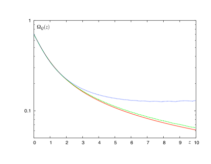
This is a crude assumption, because the value of $w$ at high $z$ will be $w_{0}+w_{1}(\log(2)-\arctan(1)+\pi/2)$ which has no reason to correspond to the high $z$ asymptote of a given tracking potential model. However, as said above, the dark energy component is completely dominated at high redshift by the energy density of matter, and the expansion is nearly insensitive to its evolution. In the end, the only thing that matters is the evolution of dark energy from the epoch when it starts to dominate. This epoch can be at redshift as high as 10. For example, in a SUGRA $\alpha=6$ modelBrax and Martin (2000) the energy density of dark energy represents 10% of the total energy density as early as redshift $z\sim 5$ (see figs. 3 and 1 ).

The parameterization, Eq. (29), is not very good at fitting the equation of state. As shown figure 3 for the example of a SUGRA $\alpha=6$ model, it reasonably agrees with the dark energy density predicted in this model. This is not the relevant comparison anyway, as we should compare the growth and distances of the different models. This is done fig. 4.

Figure 4: Comparison between real tracking models and their approximated version using Eq. (29). Top panel present the comoving distances, bottom the growth of structure. The lines plain line is a SUGRA $\alpha=6$ model, the dashed one, SUGRA $\alpha=11$ and the dotted a Ratra-Peebles, $\alpha=4$ model. The discrepancy on the angular distances computed with the real model and our parameterization is below the percent up to $z=4$. The discrepancy for the linear growth if of order 3 % up to the recombination. Our approximated formula with its very small number of parameters gives a good approximation of the quantities on which is computed the weak lensing effect.

The agreement with the explicit tracking models we tested is around 3%. We will assume that this order of magnitude of the error holds for any other tracking model.

We use this parameterization in our analysis. Although it is a ad hoc choice, it conveys most of the feature of a tracking model, and fits them, at least at the level of the growth of structure and the cosmological distances. It also has the advantage to be described by only two parameters, $w_{0}$ and $w_{1}$. We have fixed the change between the log and tan branches to $z_{c}=1$. Small variations of $z_{c}$ translate into small modifications of the growth of structure. For example, taking $z_{c}=1.5$ translates into one percent modification in $D_{+}/a$, comparable with the error on the modeling. Of course, since we are only interested to lensing effect to redshift around 1, it leads to negligible modifications in the cosmological distances and the projection effect . Finally, since the parameterization (29) admits Eq. (24) as its Taylor expansion, our results are directly comparable with the well advertised SNIa ones Goliath et al. (2001).

II Results

We perform a maximum likelihood analysis of the aperture mass statistic for a set of dark energy models. The method is well known and has been formerly described in Van Waerbeke et al. (2002). Section II.1 describes the models and surveys that will be investigated. Finally, we present section II.2 the numerical results and a discussion on the degeneracy between the parameters.

II.1 Parameter estimation

We know from previous studies that the gravitational lensing by large scale structures depends mainly on four parameters: the matter energy density $\Omega_{0}$, the mass power spectrum normalisation $\sigma_{8}$, its slope, and the redshift of the sources Schneider et al. (2002). As described above, we can safely ignore modification to the Cold Dark Matter transfert function Bardeen et al. (1986) due to dark energy. We thus use it and describe the slope of the power spectrum by the parameter $\Gamma$.

The lensing effect is also sensitive to other parameters, but to a lower extend. Therefore when studying the impact of the dark energy on cosmic shear, one has to incorporate the effect of the main parameters as well. We highlighted above that in the linear regime at least, dark energy variation should be degenerated with the normalization of the power spectrum. By keeping the main parameter we will be able to test other possible degeneracies.

We assume that one of the main parameters is known. Indeed, the forthcoming lensing surveys are supposed to provide an accurate measurement of the distribution of the sources from photometric redshifts. Moreover, the redshift dependence is very similar to the $\sigma_{8}$ dependence. Hence, we will assume $z_{s}$ known. A slight error on its value can be translated in our result in broader $\sigma_{8}$ constraint.

Our set of free parameters is chosen as ${\textrm{p}}=(w_{0},w_{1},\Omega_{0},\sigma_{8},\Gamma)$. We deliberately choose a flat prior. The current CMB results are in very good agreement with a flat geometry Spergel et al. (2003).

We compute the likelihood ${\mathcal{L}}({\textrm{p}}|{\bf d})$, where the data vector ${\bf d}$ is the aperture mass $\langle M_{\textrm{ap}}^{2}\rangle$ as function of scale:

$${\mathcal{L}}={\frac{1}{(2\pi)^{n/2}\left|{\bf S}\right|^{1/2}}}\leavevmode\nobreak\ \exp{\left[-{\frac{1}{2}}\left({\textrm{{\bf d}-{\bf s}}}\right)^{T}{\bf S}^{-1}\left({\textrm{{\bf d}-{\bf s}}}\right)\right]},$$ (30)

where ${\bf s}$ is the fiducial model vector and ${\bf S}:=\langle\left({\textrm{{\bf d}-{\bf s}}}\right)^{T}\left({\textrm{{\bf d}-{\bf s}}}\right)\rangle$ is the covariance matrix. The covariance matrix is computed following the method described in Schneider et al. (2002) assuming the Gaussian field approximation. In this work we are interested in two surveys: one is the ground based Canada France Hawaii Telescope Legacy Survey , and the other the spatial Super-Novae Acceleration Probe . The observational properties of the lensing survey associated with these two projects are summarized in table 1.

Figure 5: Aperture mass variance as function of scale for model3 (solid) and model2 (dashed), for the CFHTLS (thick bottom lines) and SNAP (thin top lines). The error bars show the statistical and sampling errors, assuming aGaussian statistic for the sampling error.

	$\bar{z}_{s}$	$\theta_{\textrm{deg}}^{2}$	$n_{\textrm{gal}}$	$\sigma_{\textrm{e}}$
CFHTLS	0.9	1790.	20.	0.44
SNAP	1.2	300.	100.	0.32

Table 1: Lensing surveys that will be part of the CFHTLS and SNAP projects (see text). Entries are source mean redshift $\bar{z}_{s}$, survey total area $\theta_{\textrm{deg}}^{2}$, source galaxy number density (per arc-min²), and intrinsic ellipticity dispersion $\sigma_{\textrm{e}}$.

For the two surveys, we selected three fiducial models (with a cosmological constant $\Omega_{\Lambda}=0.7$):

• model1: ${\textrm{p}}_{1}=(-1,0,0.3,0.9,0.24)$

• model2: ${\textrm{p}}_{2}=(-0.8,0,0.3,0.9,0.24)$

• model3: ${\textrm{p}}_{3}=(-0.8,0.32,0.3,0.9,0.24)$

The first model is a pure cosmological constant case. Second is a minimal dark energy model with no variation of the equation of state. This type of model is widely used in the literature. From the discussion of section I.4, it is expected that this kind of model under-evaluate greatly the effect of a varying EOS with identical final value. Last model has a varying EOS. The value of $w_{1}$ has been choose so as to agree with a $\alpha=6$ SUGRA model. It correspond to a strongly evolving equation of state model. Models with a smaller $w_{1}$ between our choices interpolate between our model2 and model3.

We also have to make a choice on the range of parameters we want to investigate. Maximum likelihood analysis with five parameters is already a computationally expensive task. It can be reduced in part by narrowing the range of the parameters and the number of points in each direction.

For the CFHTLS analysis, it is expected that we will mildly constrain the parameters. We thus used a relatively sparse grid and relatively wide parameter ranges. The matter density $\Omega_{0}$ will be allowed to vary between 0.1 and 0.5, while $\sigma_{8}$ will be free between 0.6 and 1.1. The choices for this two parameters are quite conservative. They allow to probe the full one sigma contour. The slope of the power spectrum is weakly constrained by the weak lensing measurement we probe its values between 0.08 and 0.4. The results below (figures 9-11) shows that this is more that enough to correctly probe the parameter space.

For SNAP, we greatly reduce the range of parameters. The precision required here forces us to increase the number of computed models, in particular in the $\Omega_{0},\sigma_{8}$ space. We thus suppose that it is enough to probe $\Omega_{0}$ between 0.28 and $0.32$, and $\sigma_{8}$ between $0.85$ and $0.95$. Nevertheless, it is expected that by the time SNAP will collect data, previous weak lensing measurements, CMB, galaxy and cluster surveys will have cut down the accuracy on this parameters to these levels. We conservatively keep a relatively wide range on $\Gamma$ ($0.1$ to $0.3$, in agreement with the results for CFHTLS).

For both models, we probed the dark energy parameter space between -1 and 0.6 for $w_{0}$ and 0 and 0.4 for $w_{1}$. Note here that as described higher, we do not take into account models with an equation of state more negative than -1. The upper bond on $w_{0}$ correspond roughly to the degeneracy expected between our target varying equation of state and a constant equation of state model (see section I.4). We do not investigate negative $w_{1}$ models. Negative $w_{1}$ models are very close to the cosmological constant case, and should be strongly degenerated with it. It is very dubious that weak lensing will be able to distinguish between them. The $w_{1}$ upper bond correspond to strongly varying equation of state. It is very difficult to reach this bond with SUGRA or Ratra-Peebles models.

II.2 Numerical results – Discussion

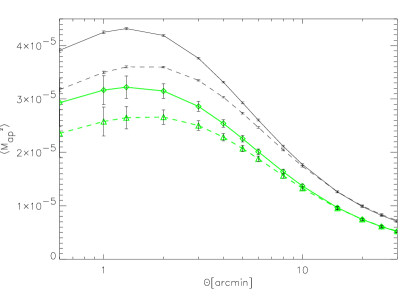
We first compute the aperture mass for our dark energy models. Figure 5 presents the results for SNAP and the CFHTLS surveys. It shows that the evolution of the dark energy can lead to a $10$ to $20\%$ effect at small scale. As emphasized section I.4, this is precisely the expected effect.

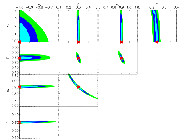
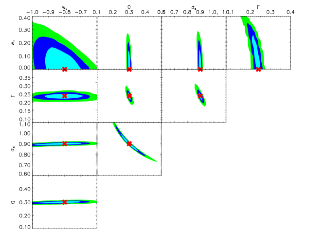
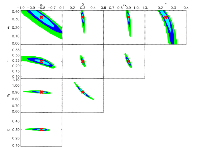
Next we perform the likelihood analysis on our target models. Figures 9, 10, and 11 show respectively the parameter predictions for the models 1, 2 and 3. All possible combinations of pairs of parameters are plotted in order to show the direction of degeneracies. On each plot, the two hidden parameters are assumed to be perfectly known. We first note the strong degeneracy between the dark energy parameters ($w_{0}$, $w_{1}$) and the other parameters. The full degeneracy between $w_{1}$ and $\Gamma$ is understood by the fact that the shape parameter describes the slope of the power spectrum, for a fixed normalisation $\sigma_{8}$. Changing $\Gamma$ will modify the ratio between linear and non-linear regime, and the scale of transition. As shown in section I.4, a change in $w_{1}$ has a similar consequence.

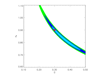
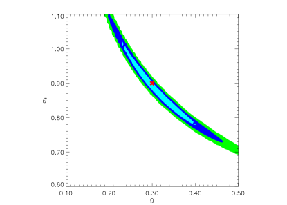
Even allowing for dark energy, the shear two points function remains a good constraint on $\Omega_{0}$ and $\sigma_{8}$. Figure 6 shows the effect of unknown dark energy parameters (marginalised on $w_{0}$ and $w_{1}$) on the measurement of $\Omega_{0}$ and $\sigma_{8}$. For the pure cosmological constant model (top panel), we see that the most probable models correspond to higher $\Omega_{0}$ and lower $\sigma_{8}$ than the fiducial model. For the model2 (bottom panel), the normalisation is underestimated. This figure shows that the width of the $\Omega_{0}$, $\sigma_{8}$ contours is not dramatically affected, but the most probable models are changed.

Figure 6: Contours in the $\Omega_{0}$, $\sigma_{8}$ space when marginalised over the quintessence $w_{0}\in[-1,-0.7]$ and $w_{1}\in[0,0.4]$. This is given for the CFHTLS experiment, left panel corresponds to model 1, and right panel to model 2.

Super-Novae luminosity surveys have a small sensitivity to the variation of the equation of state. In particular, it is expected that without a strong prior on $\Omega_{0}$ they cannot provide much information on $w_{1}$ Astier (2001); Maor et al. (2001); Goliath et al. (2001). The question is whether the shear two points function also suffers from this kind of limitation or not. Figure 7 and 8 show the predictions for $w_{0}$ and $w_{1}$, respectively for the CFHLS and SNAP observations. The left panels correspond to the contours obtained with a perfect knowledge of $\Omega_{0}$, $\sigma_{8}$ and $\Gamma$. The middle panels are for a known $\Gamma$, but marginalised over $\Omega_{0}$ and $\sigma_{8}$. The right panels are for known $\Omega_{0}$ and $\sigma_{8}$, and marginalised over $\Gamma$. The top panels are for model 2, and the bottom panel for model 3. The important result here is that the marginalisation over $\Omega_{M}$ and $\sigma_{8}$ do not increase too much the width of the contours, it only restores a degeneracy between $w_{0}$ and $w_{1}$.

Figure 7: CFHTLS constraints with lensing alone on $w_{0}$ and $w_{1}$. Top panels: model2, bottom panels: model3. Left plot is assuming all other parameters are known (see Figure 10 and 11). Middle plots is when the mean density and the power normalisation are marginalised (flat prior) over $\Omega_{0}\in[0.1,0.5]$ and $\sigma_{8}\in[0.6,1.1]$. The right plots show the contour for the marginalisation $\Gamma\in[0.1,0.4]$.

Figure 8: Same as Figure 7for the SNAP survey. The marginalisation is performed over the intervals $\Omega_{0}\in[0.28,0.32]$ and $\sigma_{8}\in[0.85,0.95]$ for the middle plots and $\Gamma\in[0.1,0.3]$ for the right plots. The line show the direction of degeneracy of the SNIa (with the supposition of a perfect $\Omega_{0}$ knowledge)

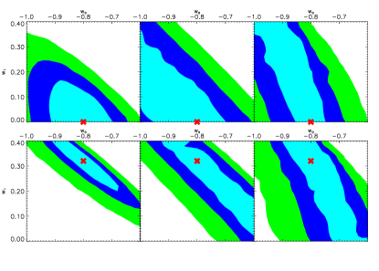
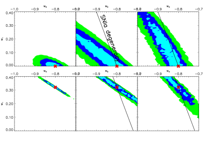
Contrary to the angular diameter distance tests, the weak lensing is sensitive to the evolution parameter $w_{1}$. The marginalisation over $\Gamma$ restores the degeneracy along a different direction, but still does not increase the contours width significantly. It means that even with a limited knowledge on external important parameters, it is still possible to constrain the quintessence, in particular when it evolves with time. In that case indeed (i.e. $w_{1}\neq 0$), the increase of the lensing signal is large enough to allow the CFHTLS observations to rule out a pure cosmological constant case. However, an accurate joint measurement of the quintessence parameters and the others is not possible using the lensing power spectrum alone, because of the strong degeneracy between $\Omega_{0}$ and $\sigma_{8}$.

This degeneracy is broken with the SNAP lensing survey: according to Figure 8, one sees that cosmic shear observations alone with the SNAP satellite, provide constraints which are competitive with the SNIa constraints from the same satellite. The expected constraints from SNIa alone, assuming a perfect knowledge of $\Omega_{0}$, is sketched on this figure (solid line). It shows that SNIa are less sensitive to $w_{1}$ than weak lensing. Therefore a combination of SNIa and cosmic shear could simultaneously probe the dark energy and its evolution. More precisely, figures 9, 10, and 11 show that the knowledge of $w_{0}$ is irrelevant for constraining $\Omega_{0}$ from cosmic shear. On the other hand, the SNIa measurements are degenerate between $w_{0}$ and $\Omega_{0}$. A combination of the two experiments provide a simultaneous measure of $w_{0}$ and $\Omega_{0}$ without the need for an external measurement of $\Omega_{0}$. We can then use the lensing constraints on $w_{0}$ and $w_{1}$ (Figures 7 and 8) to estimate the dark energy evolution $w_{1}$. In fact even a poor knowledge of $\Omega_{0}$ can be tolerated; we known from Goliath et al. (2001) that a marginalisation over $\Omega_{0}$ of the SNIa measurements increases the $w_{0}$, $w_{1}$ contours perpendicularly to the increase of the same contours from cosmic shear with poor knowledge on $\Omega_{0}$ (Figures 7 and 8, middle panels). Adding the cosmic microwave background over-constrains the parameter space, because the contours in the $\Omega_{0}$, $w_{0}$ space are ’perpendicular’ to the SNIa and cosmic shear constraints Spergel et al. (2003). Weak lensing, cosmic microwave background and SNIa provide therefore an ideal set of complementary experiments for constraining the dark energy beyond the constant energy density case Frieman et al. (2003), because weak lensing measurement breaks the degeneracy with the dark energy evolution.

Earlier work has shown that cosmic shear provides also independent constraints on $\Omega_{0}$ from the measurement of high order statistics of the convergence Pen et al. (2003); Bernardeau et al. (2003, 2002); van Waerbeke et al. (1999). Dark energy modifies mildly this picture. At the level of the quasi-linear regime, it only affects the three points function of the convergence field through the projection effect Benabed and Bernardeau (2001). The modifications are expected to be more important at small scales Hui (1999). One can see from Figure 9, 10, and 11 that this additional information is not necessary, given the degeneracy among $w_{0}$ in the ($w_{0}$, $\Omega_{0}$) space. However, such external constraint could be very helpful to pin down the degeneracy with $\sigma_{8}$, and consequently to reduce the degeneracy between $w_{0}$ and $w_{1}$, helping to narrow the constraint on $w_{1}$.

Figure 9: Constraints obtained with the CFHTLS survey for a cosmological constant model (model1). We assumed strong prior for the hidden (not shown) parameter on each plot. The cross represents the fiducial model.

Figure 10: Same as Figure 9for a quintessence, non evolving, model2 (see table 1)

Figure 11: Same as Figure 10 for an evolving dark energy model (model3).

III conclusion

We investigated the possibility to constrain the evolution of dark energy evolution from measurements of the gravitational lensing by large scale structures. We used the fact that the non-linear growth rate of structures is significantly affected. This is a consequence of an earlier influence of dark energy on the expansion of the Universe. It was found that the cosmic shear effect is an ideal probe of the evolution of dark energy, in opposition with experiments based on angular diameter distances like SNIa and cosmic microwave background, which are better suited to measure the “constant” part of dark energy equation of state (in a particular parametrization). The degeneracy with other parameters ($\Omega_{0}$, $\sigma_{8}$ and $\Gamma$) restore a degeneracy between $w_{0}$ and $w_{1}$, but the width of the contours in that space are slightly affected. Therefore a linear combination of $w_{0}$ and $w_{1}$ is well measured using weak lensing, even with a poor knowledge on $\Omega_{0}$ and $\sigma_{8}$.

It is generally believed that the measurement of the dark energy equation of state parameter as a constant is such a difficult task, that we should not even dream to measure its evolution. We have shown here, for a class of models, that the sensitivity of the large scale structures to a simple evolution parameter $w_{1}$ is as easy (or difficult!) as $w_{0}$ to measure. Consequently, we found out that a combination of cosmic shear, SNIa and cosmic microwave background provide orthogonal constraints of the parameters $w_{0}$, $w_{1}$ and $\Omega_{0}$, which opens great opportunities to probe non-trivial models of dark energy. For the set of models studied here, we found that these three experiments over constrain these parameters.

One should note that the difference in the amplitude of the cosmic shear signal between model 2 ($w_{0}=-0.8$, $w_{1}=0$) and model 3 ($w_{0}=-0.8$, $w_{1}=0.32$), at scales below $5^{\prime}$ reaches $10\%$. This is large compared to the statistical errors of the CFHTLS and SNAP surveys. However, it is yet within the limits of the Point Spread Function (PSF) correction and non-linear modeling accuracies Van Waerbeke et al. (2002). If one wants to measure the dark energy evolution as proposed here, it is clear that we need to perform ray-tracing simulations for the class of models we want to investigate, in order to calibrate the non-linear modeling Smith et al. (2002). The PSF correction is an entirely different issue, which is not discussed here, but there is good hopes to be able to reduce the systematics level by a factor of 5 to 10 Hoekstra (in preparation), which should be enough for our purpose here.

Redshift degeneracy was not discussed, but it is not different from the $\sigma_{8}$ and the $\Omega_{0}$ degeneracies. What has been said for these parameters also applies to the source redshift. In the future, photometric redshifts will provide accurate source redshift measurements, as we do not need an accurate redshift for each lensed galaxy.