Tests of Statistical Significance and Background Estimation in Gamma Ray Air Shower Experiments.

Abstract

In this paper we discuss several methods of significance calculation and point out the limits of their applicability. We then introduce a self consistent scheme for source detection and discuss some of its properties. The method allows incorporating background anisotropies by vetoing existing small scale regions on the sky and compensating for known large scale anisotropies. By giving an example using Milagro gamma ray observatory we demonstrate how the method can be employed to relax the detector stability assumption. Two practical implementations of the method are discussed. The method is universal and can be used with any large field-of-view detector, where the object of investigation, steady or transient, point or extended, traverses its field of view.

1 Introduction

The problem of evaluation of statistical significance of observations when searching for gamma ray sources using air shower experiments remains one of highest importance. The emission from a source would appear as an excess number of events coming from the directions of the candidate over the background level. The difficulty arises because the signal to background ratio as registered by the detectors in this energy range is often quite unfavorable, requiring careful examination of data.

In this paper, we expand on the usually adopted procedure of the significance calculation described by Li and Ma (1983), in particular on the conditions of its applicability. The prescription relies on the knowledge of the expected background level, methods of estimation of which are reviewed in Alexandreas et al. (1993). However, the standard significance calculation method is not compatible with these methods of background estimation. In this paper we introduce a self consistent scheme for a source detection and discuss some of its properties. The method is applicable to point and extended source searches as well as to searches for transient phenomena. We show how practical problems specific to an experiment can be incorporated into the method.

The methods described in this paper were developed for, and applied in two gamma ray searches (Fleysher, L., 2003; Fleysher, R., 2003) using the Milagro water Cherenkov air shower detector (Atkins et al., 2000).

2 Gamma ray astronomy using the air shower technique.

A typical air shower detector registers particles from air showers that survive to the ground level. The recorded information is used to provide the direction of the incident primary particle and perhaps provide some information on its energy and type. Among the particles entering the Earth’s atmosphere gamma rays present a very small fraction, often less that $10^{-3}$. Most of the air showers are induced by charged cosmic rays that form a background to the search for gamma initiated showers from a source. Special techniques and algorithms have been developed to suppress this background in order to increase the sensitivity to gamma primaries. These, however, are limited due to similarities of the cascades produced by primaries of both types. The application of these techniques helps but does not solve the problem of gamma ray source detection in the presence of a background. Therefore, one of the problems in gamma ray astronomy using air shower technique is to be able to determine the level of background (Alexandreas et al., 1993). This problem is rather difficult if one tries to calculate it from the first principles, because it would require exact knowledge of the details of the detector operation, its sensitivity which may depend on voltages, temperature, properties of atmosphere and direction reconstruction algorithms. The problem is solved by measuring the background level using the same instrument.

Thus, in a typical experiment, two measurements are performed — one corresponding to the observation of the candidate (so called on-source) and the other is the measurement of the corresponding background level (so called off-source observation). Then, a decision is made as to the plausibility of the existence of the source. Because the results of the on- and off-source observations represent random numbers drawn from their respective parent distributions, the question of the existence of the source is the question of whether the numbers are drawn from the same or different parent distributions. It is addressed by a hypothesis test.

3 Li Ma statistic.

Many statistical tests have been used to test the null hypothesis of the absence of a source given two independent counts $N_{1}$ from the on-source and $N_{2}$ from the off-source regions accumulated during time periods $t_{1}$ and $t_{2}$ respectively with all other conditions being equal. An improvement was proposed by Li and Ma (1983) and is based on the test statistic:

$$U=\frac{N_{1}-\alpha N_{2}}{\sqrt{\alpha(N_{1}+N_{2})}}\;\;\;\;\alpha=t_{1}/t_{2}>0$$ (1)

Because each event carries no information about another, each of the observed counts can be regarded as being drawn from a Poisson distribution with some value of the parameter (adjusted for the duration of observation). The motivation provided by the authors is that the numerator may be interpreted as the excess number of events from source over the expected background and denominator is the maximum likelihood estimate of the standard deviation of the numerator given that the null hypothesis is true.

It has been argued by the authors (Li and Ma, 1983) that for the case of large $N_{1,2}$ $(N_{1,2}>10)$, and if the null hypothesis is true, the distribution of $U$ becomes Gaussian with zero mean and unit variance. This statement is based on the well known fact that Poisson distribution approaches that of Gaussian for large values of parameter $\mu$:

$$P_{\mu}(n)=\frac{\mu^{n}}{n!}e^{-\mu}\approx\frac{1}{\sqrt{2\pi\mu}}e^{-{(n-\mu)^{2}}/{2\mu}}$$

For a measured value $u$ of $U$, the calculation of the $p$-value (which we denote by $\xi$) becomes simple:

$$\xi=\frac{1}{\sqrt{2\pi}}\int_{u}^{+\infty}e^{-{x^{2}}/{2}}dx$$

when looking for a source and

$$\xi=\frac{1}{\sqrt{2\pi}}\int_{-\infty}^{u}e^{-{x^{2}}/{2}}dx$$

when looking for a sink.

The null hypothesis is rejected with significance $\xi_{c}$ if $\xi<\xi_{c}$. The significance $\xi_{c}$ is set in advance, before the test is performed and its choice is based on the penalty for rejecting the null hypothesis when it is true. (Scientific false discoveries should not happen very often, and thus the significance is usually selected as $\xi_{c}=10^{-3}$.) Because of the one-to-one correspondence between $\xi$ and $u$, the significance of a measurement can be quoted in the units of $U$.

3.1 Conditions of applicability of Li Ma statistic.

(a) Values of $N_{1}$ and $N_{2}$ are drawn from Poisson distribution with averages equal to 500 and 5000 respectively ($\alpha=0.1$). According to equation (3.1), $u_{b}\ll 5.3$.

(b) Values of $N_{1}$ and $N_{2}$ are drawn from Poisson distribution with averages equal to $15\cdot 10^{5}$ and $15\cdot 10^{6}$ respectively ($\alpha=0.1$). According to equation (3.1), $u_{b}\ll 20.3$.

Figure 1: Distributions of statistic $U$ (equation 1) obtained in two runs of Monte Carlo simulations. Parameters of the best fit to a Gaussian distribution are listed in the box. The two curves should agree in the $u_{b}$-neighborhood around zero. The number of entries in each run (about $10^{9}$) was chosen to provide reasonable accuracy in the region plotted.

(a) Values of $N_{1}$ and $N_{2}$ are drawn from Poisson distribution with averages equal to 500 and 5000 respectively ($\alpha=0.1$). According to equation (3.1), $u^{\prime}_{b}\ll 5.3$.

(b) Values of $N_{1}$ and $N_{2}$ are drawn from Poisson distribution with averages equal to $15\cdot 10^{5}$ and $15\cdot 10^{6}$ respectively ($\alpha=0.1$). According to equation (3.1), $u^{\prime}_{b}\ll 20.3$.

Figure 2: Distributions of statistic $U^{\prime}$ (equation 3) obtained in two runs of Monte Carlo simulations similar to that presented in figure 1.

When the null hypothesis is true, the distribution of statistic $U$ (equation 1) approaches the normal distribution in the limit of large numbers. Indeed, substituting the factorial in the Poisson distribution using the Stirling formula $n!\approx\sqrt{2\pi n}\;n^{n}e^{-n}$, one obtains:

$$P_{\mu}(n)=\frac{\mu^{n}}{n!}e^{-\mu}\approx\frac{1}{\sqrt{2\pi n}}\left(\frac{e\mu}{n}\right)^{n}e^{-\mu}$$

or

$$\ln\left(P_{\mu}(n)\sqrt{2\pi n}\right)\approx n\left(1-\ln\frac{n}{\mu}\right)-\mu$$

Expanding the right hand side into Taylor series in $n$ in the vicinity of $\mu$, denoting $\delta=(n-\mu)$ and keeping first two non-zero terms, we obtain:

$$P_{\mu}(n)=\frac{\mu^{n}}{n!}e^{-\mu}\approx\frac{1}{\sqrt{2\pi\mu(1+\delta/\mu)}}e^{-{\delta^{2}}/{2\mu}}\cdot e^{{\delta^{3}}/{6\mu^{2}}}$$

Thus, it is seen that the Poisson distribution approaches that of Gauss in a narrow region around its mean: $\left|{\delta^{3}}/{6\mu^{2}}\right|=\left|{(n-\mu)^{3}}/{6\mu^{2}}\right|<<1$ with $\mu\geq 6$. Substituting $n$ with $N_{1,2}$ and $\mu$ with corresponding estimates of $\mu=(N_{1}+N_{2})t_{1,2}/(t_{1}+t_{2})$ we obtain the region around zero $|u|<|u_{b}|$ where the distribution of statistic $U$ is approximately normal. That is, for

$$|u|<|u_{b}|<<$$

$$\min \left(\sqrt[6]{36\alpha(1+\alpha)^{2}(N_{1}+N_{2})},\;\right.$$

$$\left.\sqrt[6]{36\alpha^{-3}(1+\alpha)^{2}(N_{1}+N_{2})}\right)$$

the error on the $p$-value $\xi$ due to this approximation does not exceed ${1}/{\sqrt{2\pi}}\;\int_{u_{b}}^{+\infty}e^{-{x^{2}}/{2}}dx$. Figure 1 shows the results of a Monte Carlo simulations for distribution of the statistic $U$. It can be seen that the distribution is approximately normal in the vicinity of zero.

By the same arguments it may be shown that within essentially the same region around zero, another statistic $U^{\prime}$

$$U^{\prime}=\frac{N_{1}-\alpha N_{2}}{\sqrt{N_{1}+\alpha^{2}N_{2}}}$$ (3)

is also distributed normally. The motivation for statistic $U^{\prime}$ is similar to that of statistic $U$ (equation 1) that the numerator may be interpreted as the excess number of events from source over the expected background but the denominator is the maximum likelihood estimate of the standard deviation of the numerator given that the alternative hypothesis is true. (The alternative hypothesis in this case is that both observations $N_{1}$ and $N_{2}$ are from Poisson distributions with unrelated means.) Although this motivation appears to be incorrect and the statistic was abandoned by Li and Ma (1983), the critical range of $U^{\prime}$ may be defined as $u^{\prime}>u^{\prime}_{0}$ for testing the null hypothesis against the presence of a source and $u^{\prime}<u^{\prime}_{0}$ for testing against the presence of a sink. Because under the conditions of applicability of Li Ma statistic (equation 3.1) statistic $U^{\prime}$ is distributed normally, the $p$-value calculation is identical to that of for statistic $U$. The figure 2 presents the results of Monte Carlo simulations of distribution of statistic $U^{\prime}$.

In general, a hypothesis test may be based on any statistic if its distribution under the null hypothesis in known.

It is interesting to note that equation (3.1) can be used to aid in the design of an experiment. Indeed, if the relative on- to off-source region exposure can be estimated before the experiment is performed, then equation (3.1) allows estimating the observation time needed to collect enough events to reach the accuracy of statistics $U$ or $U^{\prime}$ compatible with the desired significance $\xi_{c}$. For example, if $\alpha\approx 0.1$ and the significance in units of $U$ is set at 3.0, then the experiment (duration of observation) has to be designed in such a way as to allow accumulation of at least $10^{5}$ events from the on-source region. If the significance is set at 5.0, then number of on-source events should be at least $10^{6}$.

4 Background estimation.

In order to be able to implement any of the above hypothesis tests, one must assure that the two measurements $N_{1}$ and $N_{2}$ are independent and that the ratio of observation times $\alpha$ is available while other conditions are equal. Indeed, examining a typical scenario of a gamma ray experiment it is seen that on- and off-source observations can be performed at the same time utilizing the wide field of view of the detector, or they can be performed at different times making measurement in the same local directions of the field of view. (Due to the Earth’s rotation, the off-source bin may present itself in the directions of local coordinates previously pointed at the source bin.) Both of these stipulations could contradict to the conditions of “being equal”: if observations are done at the same time, then non-uniformity in the acceptance of the array to air showers due to detector geometry must be compensated for; if observations are done at different times, then any time variation in detector operation must be addressed. Under these varying conditions, the meaning of the parameter $\alpha$ must be changed to the effective ratio of exposures of the bins. The mechanism of such an equalization and $\alpha$ determination is called background estimation. The name is due to interpretation of the second term of the numerator of equation (1) as the expected number of background events in the source region: $N_{b}\equiv\alpha N_{2}$. Correspondingly, the number of events $N_{1}$ obtained from the direct source observation will be denoted $N_{s}\equiv N_{1}$. Below we consider two methods of background estimation: direct integration and time swapping.

4.1 Isotropy and stability assumptions.

A widely accepted method of background estimation (Alexandreas et al., 1993) recognizes that usually no major changes in the detector configuration are made on short time scales and takes advantage of the rotation of the detector with the Earth which sweeps the sky across the detector’s field of view. It also recognizes that most air showers detected are produced by charged cosmic rays. Because of their charge and because of the presence of random magnetic fields in the interstellar medium, the cosmic ray particles lose all memory of their initial directions and sites of production, and can be regarded as forming isotropic radiation. Detector configuration stability implies that the acceptance of the detector is time independent although variations in the overall rate of detected events are allowed. (An example of such rate variations could be an event rate decrease caused by a temporary data acquisition system overload.) Therefore, the average number of detected events as a function of local coordinates $x$ and time $t$ on the short time scale can be written in the form:

$$dN(x,t)=G(x)\cdot R(t)\;dxdt$$ (4)

Here $R(t)$ is overall event rate, $G(x)$ — acceptance of the array such that $\int_{field\;of\;view}G(x)\;dx=1$. The local coordinates $x$ could be either hour angle and declination or zenith and azimuth. The average number of background events expected in the source bin, is then given by

$$N_{b}=\int\int(1-\phi(x,t))\;G(x)\;R(t)\;dxdt$$ (5)

where $\phi(x,t)$ is equal to zero if $x$ and $t$ are such that they translate into inside of the source bin, and is one otherwise. The isotropy and stability assumptions (equation 4) become part of the null hypothesis being tested.

4.2 Direct integration method.

The direct integration method of source detection is based on isotropy and stability assumptions (equation 4) and is the method where the integration of equation (5) is performed numerically by discretizing both $G(x)$ and $R(t)$ on a fine grid and replacing integrals by sums. The significance test is based on either statistic (1) or (3). The acceptance and the event rate are estimated by histogramming local coordinates $x$ and event times $t$ of the events collected during integration time period from the entire sky. The fluctuations in $N_{b}$ are dominated by the ones in $G(x)$ because the event rate $R(t)$ is collected from the entire sky and may be deemed as known to high precision. In this scheme, the source region defined by $\phi(x,t)$ also gets discretized, therefore, source count $N_{s}$ must be obtained using the same discretized definition of the source region. Extending the time integration window is equivalent to increasing exposure to the off-source bin, which leads to decreasing value of $\alpha$ and improved sensitivity. The assumption (4), however, must hold during the entire integration period placing a constraint on the maximum size of the off-source bin. The time integration window is limited by 24 hours of sidereal day.

4.2.1 Eliminating on-source events from background estimation.

The realization of the direct integration method just described includes on-source events $N_{s}$ in the calculation of expected background $N_{b}$ (via $G(x)$ and $R(t)$). This, however, is inconsistent with their independence required by Li Ma statistic (equation 1) and was already recognized in (Alexandreas et al., 1993). An extreme example would be the case of sighting of the North Celestial Pole. There, the source does not present any apparent motion in local coordinates because it lies on the axis of rotation of the Earth. The off-source bin does not exist, the off-source count $N_{2}$ and the ratio of exposures $\alpha$ are not defined and the measurement can not be performed using isotropy and detector stability assumptions (equation 4). In the framework of the direct integration method, however, the background $N_{b}$ is guaranteed to be estimated exactly equal to $N_{s}$ and therefore $U\equiv 0$. This is clearly unsatisfactory.

In order to be able to use either of the statistics (1) or (3) the events from the source bin should be excluded from the background estimation. However, simply removing all of these events from the procedure will destroy its foundation that the lists of local coordinates and times represent samples from $G(x)$ and $R(t)$ respectively. A solution to this problem follows.

Denote by $\psi(x,t)$ a function similar to $\phi(x,t)$ which defines the region of the sky events from which are to be excluded from the background estimation. The excluded region should contain the candidate source bin, but is not limited to it. Also denote by $N_{out}(x,t)$ the number of detected events originating from outside of the excluded region, and $R_{out}(t)$ their total event rate, then it is readily seen that

$$dN_{out}(x,t)=\psi(x,t)G(x)R(t)\;dxdt$$

Integrating this equation with respect to $t$ and $x$ a system of equations on unknown $G(x)$ and $R(t)$ is obtained ($N_{out}(x)$ and $R_{out}(t)$ are available experimentally):

$$\left\{\begin{array}[]{lcl}N_{out}(x)&=&G(x)\int\psi(x,t^{\prime})\cdot R(t^{\prime})\;dt^{\prime}\\ R_{out}(t)&=&R(t)\int\psi(x^{\prime},t)\cdot G(x^{\prime})\;dx^{\prime}\end{array}\right|$$ (6)

The numerical solution of these integral equations provides $R(t)$ and $G(x)$ based on data $N_{out}(x)$ and $R_{out}(t)$ from the outside of the excluded region to be used in equation (5). The situation is illustrated on figure 3. The heavily shaded area is the outside of the excluded region bounded by $\psi(x,t)$ in its discrete form, events from which may be used for the off-source observation. The region of interest, the on-source region, is defined by some other conditions $\phi(x,t)$ which are irrelevant for the background equations (6) as long as it is contained in the excluded region.

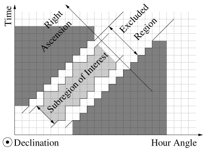
Figure 3: To the formulation of background equations (6).

It can be noted that both $G(x)$ and $R(t)$ enter into equations (6) and (5) only as a product $G(x)\cdot R(t)$, therefore, normalization of either of them does not make any difference as long as the product is preserved. Also, if there are points $\{x_{0}\}$ in the local coordinates which are always inside the excluded region, which may happen if the detector was operational during a short time period and/or the excluded region was large, (that is $\psi(\{x_{0}\},t)=0,\;\forall t$) then $N_{out}(\{x_{0}\})\equiv 0$ and the first equation of (6) becomes:

$$0=G(\{x_{0}\})\cdot 0$$

leading to $G(\{x_{0}\})$ and integral in equation (5) being undefined. On-source events with local coordinates from these regions must be discarded as having no corresponding background estimate. It is thus seen that the method entails that the second, off-source region is defined by the regions of the local sky which have the opportunity to present themselves into the directions of the source region due to the Earth’s rotation during the time period of integration. Different parts of the source region have different corresponding off-source regions. This leads to the ratio of exposures of on- and off-source regions $\alpha$ that is dependent on the local coordinates $x$:

$$\alpha(x)=\frac{N_{b}(x)}{N_{out}(x)}=\frac{\int(1-\phi(x,t))R(t)dt}{\int\psi(x,t)R(t)dt}$$

The off-source region corresponding to a given on-source region $\phi(x,t)$ is not a celestial bin, it is a set of local directions with $\alpha(x)>0$. Because the measurements made from different local directions $x$ are independent, all measurements can be combined to obtain the compound statistic $U$:

$$U=\frac{\sum_{x}N_{s}(x)-\sum_{x}N_{b}(x)}{\sqrt{\sum_{x}\alpha(x)N_{s}(x)+\sum_{x}N_{b}(x)}}$$

or

$$U=\frac{N_{s}-N_{b}}{\sqrt{\sum_{x}\alpha(x)N_{s}(x)+N_{b}}}$$

The described method is the integration scheme which is based on the direct integration method and which properly estimates the ratio of exposures $\alpha(x)$ and accounts for the source events.

The importance of the source region exclusion is illustrated on figure 4 where results of the computer simulations for a Galactic plane observation is presented. Detection of an extended source such as Galactic plane presents a difficult example because the ratio of on- and off-source exposures $\alpha(x)$ varies dramatically over the area of the source. The figure shows the excess number of events $(N_{s}-N_{b})$ extracted from a simulated galactic signal as a function of Galactic latitude. The excess is recovered correctly by the modified method (equations 5 and 6) proposed here (figure 4(b)) compared to the standard direct integration method (equation 5) (figure 4(a)). Use of the standard method would lead to a 25% loss in both the excess number of events and in value of statistic $U$ which are recovered by the modification.

(a) Excess number of events $(N_{s}-N_{b})$ as a function of Galactic Latitude. Source region is not excluded.

(b) Excess number of events $(N_{s}-N_{b})$ as a function of Galactic Latitude. The region of $\pm 7^{\circ}$ around Galactic equator is excluded from background estimation.

Figure 4: Plots showing the results of Monte Carlo simulations with uniform Galactic signal flux being 0.0088 that of background in the region of $\pm 5^{\circ}$ around the Galactic equator. The expected Galactic bin content is about 205000.

4.3 Time swapping method.

In the time swapping method of source detection the integration of equation (5) is performed by means of Monte Carlo, which leads to:

$$N_{b}=\frac{N_{0}}{N}\sum_{i=1}^{N}(1-\phi(x_{i},t_{i}))=\frac{1}{\beta}\sum_{i=1}^{N}(1-\phi(x_{i},t_{i}))$$ (7)

where $N$ generated events $(x_{i},t_{i})$ are distributed according to joint probability density $G(x)\tilde{R}(t)$ with $\tilde{R}(t)=R(t)/N_{0}$, $N_{0}$ being the total number of events detected during integration time window. A list of all coordinates of the detected events is regarded as a sample from the $G(x)$ distribution, while a similar list of all times as the one from $\tilde{R}(t)$. Therefore, sample from $G(x)\tilde{R}(t)$ distribution can be generated from the data by randomly associating an event’s local coordinate $x$ with another event’s time $t$ among the pool of detected events. The so created coordinate-time pair is called a generated event. The accuracy of Monte Carlo integration increases with the number $N$ of generated events. In the time swapping method, the function $\phi(x,t)$ defining the source region does not have to be discretized as it had to be in the direct integration method.

Here, acceptance $G(x)$ and event rate $R(t)$ must be solutions of the equations (6) to account for on-source events. In practice, Monte Carlo integration is performed by substituting each real event’s arrival time by a new time from the list of registered times of collected events in a finite time window. This is why the method is referred to as time swapping method. The swapping is repeated $\beta$ times per each real event, $\beta$ typically being around 10. The event rate $R(t)$ is considered to be constant on the very short time scale and therefore is saved as a histogram. Generated event times are drawn from it. The sample from $G(x)$ is generated using events from the outside of the excluded region and should contain $N(x)=G(x)\int R(t)dt$ events with given local coordinates $x$. However, the number of events available is $N_{out}(x)=G(x)\int\psi(x,t)R(t)dt$. Therefore, instead of swapping each event $\beta$ times, missing events are created by choosing actual number of swaps from a Poisson distribution with parameter $(1+\alpha^{\prime}(x))\beta$ where

$$1+\alpha^{\prime}(x)=\frac{G(x)\int R(t)dt}{G(x)\int\psi(x,t)R(t)dt}=\frac{G(x)\int R(t)dt}{N_{out}(x)}$$

The significance calculation has to reflect the fact that the time swapping method is a Monte Carlo integration and thus introduces additional fluctuations in the estimate of $N_{b}$. The integration error reduces as the number of generated events increases or equivalently as $\beta$ increases and the fluctuations in $N_{b}$ approach that of the direct integration method. Use of statistic $U^{\prime}$ (equation 3) provides a transparent way of including these additional fluctuations. It can be shown (Fleysher, R., 2003) that the statistic $U^{\prime}$ within framework of time swapping must be substituted by

$$U^{\prime}(x)=\frac{N_{s}-N_{b}}{\sqrt{N_{s}+\sum_{x}\alpha(x)N_{b}(x)+N_{b}/\beta}},$$ (8)

$$\alpha(x)=\frac{N_{b}(x)}{N_{out}(x)}$$

The fact that the source region defined by $\phi(x,t)$ does not have to be discretized is the advantage of the time swapping method. Otherwise, it is based on the same assumptions as the direct integration method: stability of the detector and isotropy of the background (equation 4).

4.4 Known anisotropies.

It was assumed in the above discussion that no anisotropy on the sky is present. This, together with the stability assumption had lead to the equation (4). In fact, if there are known sources on the sky, then the number of registered events is given by:

$$dN(x,t)=(1+S(x,t))\cdot G(x)\cdot R(t)\;dxdt$$ (9)

where $S(x,t)$ describes the strength of the sources as function of local coordinates and time.

For example, the Crab nebula is known to emit gamma rays in the TeV energy region (Weeks et al., 1989; Atkins et al., 2003). Because the anisotropy function $S(x,t)$ is not known, the region around the Crab has to be excluded from the background estimation even if the nebula is not the subject of investigation.

Another, more dramatic example is given by two known cosmic-ray sinks on the sky: the Sun and the Moon (Samuelson, 2001). Not only do they present a source of anisotropy, they also traverse the sky, blocking on their way potential candidates and perturbing on-source count $N_{s}$ as well as $N_{b}$. This can be handled by vetoing certain size regions around the objects, that is treating them as part of the excluded region during integration (equations 5 and 6) and disregarding events if they fall within the veto region when counting on-source events $N_{s}$. In other words, if $\nu(x,t)$ is the function describing the veto region where it is equal to zero and equal to one everywhere else, then excluded region $\psi(x,t)$ and source region $\phi(x,t)$ have to be redefined as:

$$\left\{\begin{array}[]{lcl}\psi(x,t)&:=&\psi(x,t)\cdot\nu(x,t)\\ \phi(x,t)&:=&1-(1-\phi(x,t))\cdot\nu(x,t)\end{array}\right|$$

In general, existing small scale anisotropies can be excluded or vetoed as described, known large scale ones have to be incorporated into the stability assumption. These will become a part of the null hypothesis being tested.

Incorporation of the improved stability assumption (9) into the framework of direct integration method is straightforward:

$$N_{b}=\int\int(1-\phi(x,t))(1+S(x,t))G(x)R(t)\;dxdt$$

The anisotropy function $S(x,t)$ must be discretized on the same grid as $G(x)$ and $R(t)$ are. In order to incorporate the improved stability assumption into the framework of time swapping method, the generated events $(x_{i},t_{i})$ must represent a sample from $(1+S(x,t))G(x)R(t)$ which can be achieved with the help of the rejection method.

4.5 Detector stability assumption re-examined.

Despite the fact that no reconfigurations to the detector on the short time scale are made, the acceptance of the array $G(x)$ depends on transmission properties of the atmosphere which may vary during the integration time window (equation 5). In this case the stability assumption (4) is violated and must be replaced by assumption (9), where $S(x,t)$ describes the atmospheric variations. Thus, atmosphere must be considered as an integral part of the detector and we refer to the phenomenon in general as detector instability. If the variations are known, they can be incorporated into background estimation as described above. The remainder of this section presents one method of determining such variations and shows how they are incorporated into S(x,t).

The test of the stability assumption would be a comparison of two acceptances $G_{i}(x)$ and $G_{j}(x)$, $i\neq j$ measured at different times $t_{i}$ and $t_{j}$. On physical grounds, a detector usually possesses a certain degree of azimuthal symmetry, so does the atmosphere, therefore acceptance is considered as function of zenith and azimuth angles $G(z,A)$. The histograms $G_{i}(z,A)$ and $G_{j}(z,A)$ can be collected from the data for a certain duration of time (for example 30 minutes) around $t_{i}$ and $t_{j}$. For the purpose of background estimation the time scale during which the stability assumption (4) holds must be ascertained. Therefore, the test is aimed at studying the difference between the distributions as function of time separation $\Delta t=t_{i}-t_{j}$.

It has to be recognized that presence of sources or large scale anisotropies on the sky and instability of the detector mimic each other, therefore, zenith and azimuth angle distributions alone are compared instead of two dimensional $G(x)$’s. The test can be implemented as a series of $\chi^{2}$ tests of $G_{i}(x)$ and $G_{j}(x)$ (yielding $\chi^{2}(t_{i},t_{j})$) and then obtaining the combined $\chi^{2}_{total}(\Delta t)$ for time separation $\Delta t=t_{i}-t_{j}$:

$$\chi^{2}_{total}(\Delta t)=\sum_{\Delta t=t_{i}-t_{j}}\chi^{2}(t_{i},t_{j})$$

The test statistic $\chi^{2}_{total}(\Delta t)$ so obtained follows a $\chi^{2}$ distribution with $m_{total}=\sum_{\Delta t=t_{i}-t_{j}}m(t_{i},t_{j})$ degrees of freedom if observed differences are of random nature only. Here $m(t_{i},t_{j})$ are the number of degrees of freedom in the corresponding $\chi^{2}(t_{i},t_{j})$ tests. The average of $\chi^{2}_{total}$ is equal to $m_{total}$ while its variance is equal to $2m_{total}$. Thus, the $\chi^{2}_{total}$ per degree of freedom should fluctuate around 1.0. Examining the dependence of $\chi^{2}_{total}$ on time separation $\Delta t$ it is possible to test the detector stability assumption and to ascertain the proper integration time window. If detector instability is recognized, care must be taken to improve the stability assumption.

4.5.1 Illustration of diurnal modulations using Milagro.

Figure 5: Results of stability assumption test with regard to zenith coordinate using Milagro data. Horizontal axis is time separation $\Delta t$ with 30 minute bins, vertical axis is corresponding ${\chi^{2}_{total}(\Delta t)}/{m_{total}(\Delta t)}$. Solid horizontal line is the expected value of one if the stability assumption holds.

Figure 5 is an example of the results of the detector stability assumption test using Milagro data with regard to zenith coordinate. (For description of Milagro please see Atkins et al. (2000).) It is seen from the plots that the degree of violation of the assumption grows with time separation $\Delta t$ as might be expected, but then it drops before growing again. This can be interpreted as presence of a periodic component which insured that two acceptances $G_{i}(z)$ and $G_{j}(z)$ separated by 24 UT hours are “closer” to each other than, say, those separated by only 12. Thus, despite the fact that no human intervention on the short time scale is made, the acceptance of the detector changes.

Because the diurnal periodicity is noted, the investigation of the modulation can be performed by comparing a particular distribution with its daily average. It was observed that the shape of the modulation ($\Delta(z)$) of the zenith distribution is approximately constant with amplitude varying from half hour to half hour. Therefore, the improved stability assumption is chosen to be of the form:

$$dN(x,t)=(1+\theta(t)\Delta(z)G(x)R(t)\;dxdt$$ (10)

where $\theta(t)$ is the amplitude of the correction at time $t$, $\Delta(z)$ is the polynomial zenith angle correction function coefficients of which are obtained from the modulation shape study, $G(x)$ is the average acceptance of the detector obtained from equations (6). The example of the correction function is shown on figure 6. The example of the average daily amplitude dependence is shown on figure 7. The value of the amplitude is typically within $\pm 4\cdot 10^{-5}$ range. The plot can also be used to justify the choice of half hour intervals for the amplitude measurement. The assumption (10) becomes part of the null hypothesis.

Figure 6: An example of the zenith correction function $\Delta(z)$ derived from Milagro data.

Figure 7: An example of the average daily dependence of the zenith correction amplitude $\theta$ derived from Milagro data.

5 Conclusions.

We have considered a typical air shower experiment conducted by means of two observations and have discussed two commonly used tests (based on statistics $U$ and $U^{\prime}$) and conditions of their applicability. A careful look at the situation where an astrophysical object traverses the large field of view of a detector had led us into the subject of background estimation. We have developed a method of background estimation which is consistent with the use of either statistics $U$ or $U^{\prime}$ and have discussed two implementations of it: direct integration and time swapping. The background estimation method is based on widely adopted assumptions of short time scale stability of the detector operation and that of isotropy of cosmic ray background. We have discussed a way to relax the short time scale stability assumption and used Milagro data to illustrate the situation where presence of zenith diurnal modulations can easily be incorporated into the background estimation method. More generally, this is also the way to incorporate known large scale anisotropies. Small scale anisotropies do not have to be known, existing ones can be handled by excluding or vetoing the regions around them. Any method based on the assumption of short time scale stability of the detector operation and that of isotropy of cosmic ray background can not be used for detection of stationary in the field of view objects.

While the methods and ideas presented in this paper were developed for a gamma-ray air shower array, we believe that the methods can also find their applications outside of the field of gamma ray astronomy. The properties of the significance test can be useful for any counting type experiment in which number of events follows Poisson distribution, the background estimation method can be used with any large field of view detector, where the object of investigation traverses the field of view, such as in solar neutrino monitors or is transient such as in SuperNovae neutrino observatories.

References

- Alexandreas et al. (1993) Alexandreas, D. E., et al. 1993, NIM, A328, 570
- Atkins et al. (2000) Atkins, R., et al. 2000, NIM, A449, 478
- Atkins et al. (2003) Atkins et, R., al. 2003, ApJ, submitted (astro-ph/0305308)
- Fleysher, L. (2003) Fleysher, L. 2003, New York University Ph.D. Thesis: Search for Relic Neutralinos with Milagro (astro-ph/0305056)
- Fleysher, R. (2003) Fleysher, R. 2003, New York University Ph.D. Thesis: Search for Gamma Ray Emission from Galactic Plane with Milagro (astro-ph/0301520)
- Li and Ma (1983) Li, T., and Ma, Y. 1983, ApJ, 272, 317
- Samuelson (2001) Samuelson, F. W. for the Milagro Collaboration 2001, in Proc. of 27-th ICRC, (Hamburg) HE130
- Weeks et al. (1989) Weeks, T. C., et al. 1989, ApJ, 342, 379