Modulational instabilities in neutrino–anti-neutrino interactions

Abstract

We analyze the collective behavior of neutrinos and antineutrinos in a dense background. Using the Wigner transform technique, it is shown that the interaction can be modelled by a coupled system of nonlinear Vlasov-like equations. From these equations, we derive a dispersion relation for neutrino-antineutrino interactions on a general background. The dispersion relation admits a novel modulational instability. The results are examined, together with a numerical example, and we discuss the induced density inhomogeneities using parameters relevant to the early Universe.

PACS numbers: 13.15.+g, 14.60Lm, 97.10Cv, 97.60Bw

, , , , and

1 Introduction

Neutrinos have fascinated people ever since they were first introduced by Wolfgang Pauli in 1931. Since then, neutrinos have gone from hypothetical to an extremely promising tool for analysing astrophysical events, and neutrino cosmology is now one of the hottest topics in modern time due to the discovery that neutrinos may be massive [1]. Because of its weak interaction with other particles, neutrinos can travel great distances without being affected appreciably by material obstacles. They can therefore give us detailed information about events taking place deep within, e.g. supernovæ. Furthermore, since the neutrinos decoupled from matter at a redshift $z$ of the order $10^{10}$, as compared to $z\simeq 10^{3}$ for photons, it is possible that neutrinos could give us a detailed understanding of the early Universe, if such a signal could be detected [2]. Massive neutrinos have also been a possible candidate for hot dark matter necessary for explaining certain cosmological observations, such as rotation curves of spiral galaxies [3]. Thus, massive neutrinos could have a profound influence on the evolution of our Universe. Unfortunately, due to the Tremaine–Gunn bound [4], the necessary mass of the missing particles (if fermions) for explaining the formation of dwarf galaxies seems to make neutrinos of any species unlikely single candidates for dark matter. As a remedy to this problem, interacting hot dark matter has been suggested [5, 6], since the interaction prevents the free-streaming smoothing of small scale neutrino inhomogeneities. Thus, dark matter in astrophysics is not only a mystery but it also plays an essential role in determining the dynamics of the universe, its large scale structures, the galaxies and superclusters. However, so far, the suggested “sticky” neutrino models have not been successful in dealing with the dwarf galaxy problem [5].

A first successful indication that neutrinos have a non-zero mass came in 1998 through laboratory experiments of atmospheric neutrinos and their oscillations [7]. Although the allowed neutrino masses encompass a wide range, it is currently believed that neutrinos have masses below 2 eV. This conclusion is furthermore supported by independent cosmological observations (see, e.g., [9]). Thus, the masses of neutrinos are indeed very small, and the classical analysis by Tremaine and Gunn would thereby indicate that neutrinos can in no way be considered as a sole candidate for dark matter. This conclusion will in this paper be re-analyzed within the electro-weak framework, where neutrino–neutrino interactions occur as a natural consequence of the theory.

Thus, in this Letter, we consider the nonlinear interaction between neutrinos and antineutrinos in the lepton plasma of the early Universe, adopting a semi-classical model. Neutrinos and antineutrinos interact with dense plasmas through the charged and neutral weak currents arising from the Fermi weak nuclear interaction forces. Charged weak currents involve the exchange of the charged vector bosons associated with the processes involving interactions between leptons and neutrinos of the same flavor, while neutrino weak currents involve the exchange of the neutral vector bosons associated with processes involving neutrinos of all types interacting with arbitrary charged and neutral particles. Asymmetric flows of neutrinos and antineutrinos in the early Universe plasma may be created by the ponderomotive force of nonuniform intense photon beams or by shock waves. Here, using an effective field theory approach, a system of coupled Wigner-Moyal equations for nonlinearly interacting neutrinos and antineutrinos is derived, and it is shown that these equations admit a modulational instability. Finally, we discuss the relevance of our results in the context of the dark matter problem, and it is moreover suggested that the nonlinearly excited fluctuations could be used as a starting point for obtaining a better understanding of the process of galaxy formation. It turns out that the short-time evolution of the primordial neutrino plasma medium in the temperature range $1\,{\rm MeV}<T<10\,{\rm MeV}$ is governed by collisionless collective effects involving relativistic neutrinos and antineutrinos.

2 Dispersion relation and the motion of neutrino bunches

As a primer, we will study the implication of the known dispersion of neutrinos on a thermal neutrino/anti-neutrino background, using the eikonal representation and the WKBJ approximation.

Suppose that a single neutrino (or anti-neutrino) moves in a Fermionic sea composed of neutrino–antineutrino admixture. The energy $E$ of the neutrino (antineutrino) is then given by (see, e.g. [10, 11])

$$E=\sqrt{p^{2}c^{2}+m^{2}c^{4}}+V_{\pm}(\bm{r},t),$$ (1)

where $\bm{p}$ is the neutrino (anti-neutrino) momentum, $c$ the speed of light in vacuum, and $m$ the neutrino mass. The effective potential for a neutrino moving on a background of it’s own flavor and in thermal equilibrium is given by [10] (see also [12, 13, 14, 15])

$$V_{\pm}(\bm{r},t)=\pm 2\sqrt{2}G_{F}(n-\bar{n}),$$ (2a)

while the potential for a neutrino moving on a background of a different flavor is

$$V_{\pm}(\bm{r},t)=\pm\sqrt{2}G_{F}(n-\bar{n}),$$ (2b)

where $G_{F}/(\hbar c)^{3}\approx 1.2\times 10^{-5}\,\mathrm{GeV}^{-2}$, $G_{F}$ is the Fermi constant, $n$ ($\bar{n}$) is the density of the background neutrinos (antineutrinos), and $+$ ($-$) represents the propagating neutrino (antineutrino). Expressions (2b) are valid in the rest frame of the background. As seen from (1) and (2b), while neutrinos moving in a background of neutrinos and antineutrinos change their energy by an amount $\sim G_{F}(n-\bar{n})$, the antineutrinos change their energy by $\sim-G_{F}(n-\bar{n})$ [16]. The extra factor of $2$ in (2a) as compared to expression (2b) comes from exchange effects between identical particles [13].

The relation (1) can be interpreted as a dispersion relation for relativistic and nonrelativistic neutrinos, with the identifications $E=\hbar\omega$ and $\bm{p}=\hbar\bm{k}$, i. e.

$$\omega=c\sqrt{k^{2}+\frac{m^{2}c^{2}}{\hbar^{2}}}+\frac{V_{\pm}}{\hbar},$$ (3)

where $\hbar$ is the Planck constant divided by $2\pi$. By using the eikonal representation (viz. $E\rightarrow\hbar\omega_{0}-i\hbar\partial/\partial t$ and $\bm{p}\rightarrow\hbar\bm{k}_{0}+i\hbar\nabla$) and the WKBJ approximation [17, 18] (viz. $|\partial{\mathnormal{\Psi}}/\partial t|\ll\omega_{0}|{\mathnormal{\Psi}}|$ and $|\nabla{\mathnormal{\Psi}}|\ll|\bm{k}_{0}||{\mathnormal{\Psi}}|$), we obtain from Eq. (3) a Schrödinger equation for slowly varying modulated (by long-scale density fluctuations) neutrino (anti-neutrino) wave function ${\mathnormal{\Psi}}(\bm{r},t)$ (i.e., neutrino bunches) (see also Ref. [16] for a similar treatment of neutrino–electron interactions)

$$i\left(\frac{\partial}{\partial t}+\bm{v}_{g}\cdot\bm{\nabla}\right){\mathnormal{\Psi}}+\frac{\hbar}{2\gamma m}\left[\nabla^{2}-\frac{(\gamma^{2}-1)}{\gamma^{2}}(\bm{n}_{0}\cdot\bm{\nabla})^{2}\right]{\mathnormal{\Psi}}-\frac{V_{\pm}}{\hbar}{\mathnormal{\Psi}}=0,$$ (4)

where $\bm{v}_{g}=c\bm{k}_{0}(k_{0}^{2}+m^{2}c^{2}/\hbar^{2})^{-1/2}$ is the group velocity of relativistic neutrinos and antineutrinos which have similar energy spectra, $\gamma=(1-v_{g}^{2}/c^{2})^{-1/2}$ is the relativistic gamma factor, $\bm{n}_{0}=\bm{k}_{0}/|k_{0}|$, and $\bm{k}_{0}$ is the vacuum wavevector. Suppose now that the neutrino bunches themselves are nearly in thermal equilibrium (to be quantified in the next section). Then, we have the case of self-interacting neutrinos and anti-neutrinos, and the densities in the potential $V_{\pm}$ is given in terms of the sums

$$n=\sum_{i=1}^{M}n_{i}=\sum_{i=1}^{M}\langle|{\mathnormal{\Psi}}_{i+}|^{2}\rangle,\,\bar{n}=\sum_{i=1}^{N}\bar{n}_{i}=\sum_{i=1}^{N}\langle|{\mathnormal{\Psi}}_{i-}|^{2}\rangle,$$ (5)

where ${\mathnormal{\Psi}}_{i+}$ and ${\mathnormal{\Psi}}_{i-}$ are the neutrino and antineutrino wave functions (with $i$ numbering the wave functions), respectively, and the angular bracket denotes the ensemble average. In this case, the relativistic neutrino and antineutrino wave packets are comoving with the background, and Eq. (4) thus yields

$$i\frac{\partial{\mathnormal{\Psi}}_{i\pm}}{\partial t}+\frac{\hbar}{2m\gamma}\left(\nabla_{\perp}^{2}+\frac{1}{\gamma^{2}}\nabla_{||}^{2}\right){\mathnormal{\Psi}}_{i\pm}-\frac{V_{\pm}}{\hbar}{\mathnormal{\Psi}}_{i\pm}=0,$$ (6)

where $\nabla_{\perp}^{2}=\nabla^{2}-(\bm{n}_{0}\cdot\bm{\nabla})^{2},\quad\nabla_{||}^{2}=(\bm{n}_{0}\cdot\bm{\nabla})^{2}$. Expressions (2a) and (5) reveal that self-interactions between relativistic neutrinos and antineutrinos produce a nonlinear asymmetric potential in Eq. (6). By further rescaling the coordinate along $\bm{n}_{0}$, Eq. (4) can finally be written as the coupled system

$$i\frac{\partial{\mathnormal{\Psi}}_{i\pm}}{\partial t}+\frac{\alpha}{2}\nabla^{2}{\mathnormal{\Psi}}_{i\pm}\mp\beta(n-\bar{n}){\mathnormal{\Psi}}_{i\pm}=0,$$ (7)

where $\alpha=\hbar/m\gamma$, and $\beta=2\sqrt{2}G_{F}/\hbar$ for neutrinos moving on the same flavor background.

Equation (7) shows that this approach can lead to some interesting effects. The case of a single self-interacting neutrino bunch shows that the formation of dark solitary structures is possible. Furthermore, the slightly more complicated case of two interacting bunches, either of the neutrino–neutrino or neutrino–anti-neutrino type, can result in splitting and focusing of the wave packets [19].

3 Kinetic description

In the preceding section, we investigated the case of a neutrino bunch close to thermal equilibrium. In general, this may of course not be the case, and Eq. (2b) must be modified. The more precise form of the potential $V_{\pm}$ for equal species due to neutrino forward scattering is given by [20]

$$V_{\pm}(t,\bm{r},\bm{p};f_{i\pm})=\pm 2\sqrt{2}\,G_{F}\int d\bm{q}\,(1-\hat{\bm{p}}\cdot\hat{\bm{q}})\left[\sum_{i=1}^{M}f_{i+}(t,\bm{r},\bm{q})-\sum_{i=1}^{N}f_{i-}(t,\bm{r},\bm{q})\right],$$ (8)

where hatted quantities denote the corresponding unit vector, and $f_{i+}(t,\bm{r},\bm{q})$ ($f_{i-}(t,\bm{r},\bm{q})$) is the neutrino (anti-neutrino) distribution function corresponding to bunch $i$. The distribution functions are defined to be normalized such that

$$n_{i}(t,\bm{r})=\int\,d\bm{q}\,f_{i+}(t,\bm{r},\bm{q}),\quad\bar{n}_{i}(t,\bm{r})=\int\,d\bm{q}\,f_{i-}(t,\bm{r},\bm{q}),$$ (9)

where $n_{i}$ ($\bar{n}_{i}$) is the number density of the $i^{\text{th}}$ neutrino (anti-neutrino) bunch.

The first thing to notice is that when the distribution is thermal, the potential (8) reduces exactly to (2a). Secondly, when the neutrinos have an almost thermal distribution, i.e. the corresponding distribution function may be expressed as (dropping the indices for notational simplicity) $f(t,\bm{r},\bm{p})=f_{0}(p)+\delta\!f(t,\bm{r},\bm{p})$, where $|\delta\!f|\ll|f_{0}|$, we obtain the following form of the potential

$$V_{\pm}(t,\bm{r},\bm{p};f_{i\pm})=\pm 2\sqrt{2}\,G_{F}\left[(n-\bar{n})-\int\,d\bm{q}\,(\hat{\bm{p}}\cdot\hat{\bm{q}})\left(\sum_{i=1}^{M}\delta\!f_{i+}-\sum_{i=1}^{N}\delta\!f_{i-}\right)\right].$$ (10)

The last term is small and may therefore be neglected, and we obtain $V_{\pm}(t,\bm{r})\approx\pm 2\sqrt{2}\,G_{F}(n-\bar{n})$, in accordance with expressions (2a), thus justifying the equation of motion (7).

Now, we define a distribution function for the neutrino states by Fourier transforming the two-point correlation function for ${\mathnormal{\Psi}}_{\pm}$, according to [21]

$${f}_{i\pm}(t,\bm{r},\bm{p})=\frac{1}{(2\pi\hbar)^{3}}\int\,d\bm{y}\,\mathrm{e}^{i\bm{p}\cdot\bm{y}/\hbar}\langle{\mathnormal{\Psi}}_{i\pm}^{*}(t,\bm{r}+\bm{y}/2){\mathnormal{\Psi}}_{i\pm}(t,\bm{r}-\bm{y}/2)\rangle,$$ (11)

where $\bm{p}$ represents the momentum of the neutrino (antineutrino) quasi-particles (note that the ensemble average was not present in the original definition [21], but has important consequences when the phase of the wave function has a random component [22]; for similar treatments of optical beams and quantum plasmas, see [22] and [23], respectively). We note that with the definition (11), the following relation holds

$$\langle|{\mathnormal{\Psi}}_{i\pm}(t,\bm{r})|^{2}\rangle=\int\,d\bm{p}\,{f}_{i\pm}(t,\bm{r},\bm{p}).$$ (12)

Thus, using (11) and (6) together with the potential (8) we obtain the generalized Wigner–Moyal equation

$$\frac{\partial{f}_{i\pm}}{\partial t}+\frac{\bm{p}}{m\gamma}\cdot\frac{\partial{f}_{i\pm}}{\partial\bm{r}}-\frac{2V_{\pm}}{\hbar}\sin\left[\frac{\hbar}{2}\left(\overleftarrow{\frac{\partial}{\partial\bm{r}}}\cdot\overrightarrow{\frac{\partial}{\partial\bm{p}}}-\overleftarrow{\frac{\partial}{\partial\bm{p}}}\cdot\overrightarrow{\frac{\partial}{\partial\bm{r}}}\right)\right]{f}_{i\pm}=0,$$ (13)

for $f_{i\pm}$, where the $\sin$-operator is defined in terms of its Taylor expansion, and the arrows denote the direction of operation. In the case of the potential (2a), the last term in the $\sin$-operator drops out, and Eq. (13) reduces to the standard Wigner–Moyal equation [21].

Retaining only the lowest order terms in $\hbar$ (i.e. taking the long wavelength limit), we obtain the coupled Vlasov equations

$$\left[\frac{\partial}{\partial t}+\left(\frac{\bm{p}}{m\gamma}+\frac{\partial V_{\pm}}{\partial\bm{p}}\right)\cdot\frac{\partial}{\partial\bm{r}}\right]{f}_{i\pm}-\frac{\partial V_{\pm}}{\partial\bm{r}}\cdot\frac{\partial{f}_{i\pm}}{\partial\bm{p}}=0.$$ (14)

The term $\partial V_{\pm}/\partial\bm{p}$ represents the group velocity. While higher order group velocity dispersion is present in (13), this is not the case in (14). Thus, information is partially lost by using the Eq. (14). Furthermore, while Eq. (14) preserves the number of quasi-particles, Eq. (13) shows that this conclusion is in general not true, i.e. the particle number in a phase-space volume is not constant, and the higher order terms $\partial^{n}V_{\pm}/\partial\bm{r}^{n}$ may moreover contain vital short wavelength information. Equations similar to (14) have been used to study neutrino–electron interactions in astrophysical contexts [11].

Suppose now that we have small amplitude perturbations on a background of constant neutrino and antineutrino densities $n_{i}=n_{i0}$ and $\bar{n}_{i}=\bar{n}_{i0}$, respectively, i.e.

$${f}_{i\pm}(t,\bm{r},\bm{p})={f}_{i0\pm}(\bm{p})+\delta\!{f}_{i\pm}(\bm{p})\exp[i(\bm{K}\cdot\bm{r}-{\mathnormal{\Omega}}t)],$$ (15)

and $|\delta\!{f}_{i\pm}|\ll|{f}_{i0\pm}|$, where $\bm{K}$ and ${\mathnormal{\Omega}}$ is the perturbation wavevector and frequency, respectively. Thus, Eqs. (13) give

$$i\left[{\mathnormal{\Omega}}-\frac{\bm{p}\cdot\bm{K}}{m\gamma}-\frac{2i}{\hbar}V_{0\pm}\sin\left(-\frac{i\hbar}{2}\overleftarrow{\frac{\partial}{\partial\bm{p}}}\cdot\bm{K}\right)\right]\delta\!{f}_{i\pm}$$

$$\qquad\qquad\qquad\qquad+\frac{2}{\hbar}\delta\!V_{\pm}\sin\left(\frac{i\hbar}{2}\bm{K}\cdot\overrightarrow{\frac{\partial}{\partial\bm{p}}}\right){f}_{i0\pm}=0,$$ (16)

where $\delta\!V_{\pm}=V_{\pm}(t,r,\bm{p};\delta\!f_{i\pm})$ and $V_{0\pm}=V_{\pm}(t,r,\bm{p};f_{i0\pm})$ from Eq. (8). Eliminating $\delta\!f_{i\pm}$ from (16), using $\delta\!V_{-}=-\delta\!V_{+}$, we have

$$\delta\!V_{+}(\bm{p}) = \frac{4\sqrt{2}\,iG_{F}}{\hbar}\int\,d\bm{q}\,(1-\hat{\bm{p}}\cdot\hat{\bm{q}})\,\delta\!V_{+}(\bm{q})$$ (17)

$$\times\left[\sum_{i=1}^{M}\frac{\sin\left(\frac{i\hbar}{2}\bm{K}\cdot\overrightarrow{\frac{\partial}{\partial\bm{q}}}\right)f_{i0+}(\bm{q})}{{\mathnormal{\Omega}}-\frac{\bm{q}\cdot\bm{K}}{m\gamma}-\frac{2i}{\hbar}V_{0+}(\bm{q})\sin\left(\frac{i\hbar}{2}\overleftarrow{\frac{\partial}{\partial\bm{q}}}\cdot\bm{K}\right)}\right.$$

$$\qquad\quad\left.+\sum_{i=1}^{N}\frac{\sin\left(\frac{i\hbar}{2}\bm{K}\cdot\overrightarrow{\frac{\partial}{\partial\bm{q}}}\right)f_{i0-}(\bm{q})}{{\mathnormal{\Omega}}-\frac{\bm{q}\cdot\bm{K}}{m\gamma}-\frac{2i}{\hbar}V_{0-}(\bm{q})\sin\left(\frac{i\hbar}{2}\overleftarrow{\frac{\partial}{\partial\bm{q}}}\cdot\bm{K}\right)}\right].$$

Assuming that $\delta\!f_{i\pm}(\bm{p})$ is a symmetric function of $\bm{p}$ implies that $\delta\!V_{\pm}$ is independent of $\bm{p}$, and Eq. (17) simplifies to the dispersion relation

$$1 = \frac{4\sqrt{2}\,iG_{F}}{\hbar}\int\,d\bm{q}\,\left[\sum_{i=1}^{M}\frac{\sin\left(\frac{i\hbar}{2}\bm{K}\cdot{\frac{\partial}{\partial\bm{q}}}\right)f_{i0+}(\bm{q})}{{\mathnormal{\Omega}}-\frac{\bm{q}\cdot\bm{K}}{m\gamma}-\frac{2i}{\hbar}\sin\left(\frac{i\hbar}{2}\bm{K}\cdot{\frac{\partial}{\partial\bm{q}}}\right)V_{0+}(\bm{q})}\right.$$ (18)

$$\qquad\quad\left.+\sum_{i=1}^{N}\frac{\sin\left(\frac{i\hbar}{2}\bm{K}\cdot{\frac{\partial}{\partial\bm{q}}}\right)f_{i0-}(\bm{q})}{{\mathnormal{\Omega}}-\frac{\bm{q}\cdot\bm{K}}{m\gamma}-\frac{2i}{\hbar}\sin\left(\frac{i\hbar}{2}\bm{K}\cdot{\frac{\partial}{\partial\bm{q}}}\right)V_{0-}(\bm{q})}\right],$$

where we have dropped the arrows indicating the direction of operation. Note that if the background distribution is thermal, $V_{0\pm}$ is independent of $\bm{p}$, and the last term in the denominators of Eq. (18) vanishes.

3.1 The one-dimensional case

The simplest way to analyse the dispersion relation (18) is to reduce the dimensionality of the problem. We therefore first look at the one-dimensional case, where we may use the identity $2\sin\left(\frac{i\hbar K}{2}\frac{\partial}{\partial p}\right)h(p)=i\left[h(p+\frac{\hbar K}{2})-h(p-\frac{\hbar K}{2})\right]$, in order to rewrite the dispersion relation (18) as

$$1 = -\frac{2\sqrt{2}\,G_{F}}{\hbar}\int dq\left\{\sum_{i=1}^{M}\frac{f_{i0+}(q+\hbar K/2)-f_{i0+}(q-\hbar K/2)}{{\mathnormal{\Omega}}-qK/m\gamma+\Delta_{+}(q)}\right.$$ (19)

$$\left.+\sum_{i=1}^{N}\frac{f_{i0-}(q+\hbar K/2)-f_{i0-}(q-\hbar K/2)}{{\mathnormal{\Omega}}-qK/m\gamma+\Delta_{-}(q)}\right\},$$

where we have introduced $\Delta_{\pm}(q)\equiv[V_{0\pm}(q+\hbar K/2)-V_{0\pm}(q-\hbar K/2]/\hbar$. In the case of mono-energetic beams, i.e. ${f}_{i0+}(p)=n_{i0}\delta(p-p_{i0})$ and ${f}_{i0-}(p)=\bar{n}_{i0}\delta(p-\bar{p}_{i0})$, Eq. (19) reduces to

$$1 = -\frac{2\sqrt{2}\,G_{F}}{\hbar}\Bigg{\{}\sum_{i=1}^{M}n_{i0}\left[-\frac{\hbar K^{2}}{m\gamma}+\Delta_{+}(p_{i0}+\hbar K/2)-\Delta_{+}(p_{i0}-\hbar K/2)\right]$$ (20)

$$\times\bigg{[}\left({\mathnormal{\Omega}}-\frac{p_{i0}K}{m\gamma}\right)^{2}-\left(\frac{\hbar K^{2}}{2m\gamma}\right)^{2}$$

$$\quad+\left({\mathnormal{\Omega}}-\frac{p_{i0}K}{m\gamma}\right)[\Delta_{+}(p_{i0}+\hbar K/2)+\Delta_{+}(p_{i0}-\hbar K/2)]$$

$$\quad+\frac{\hbar K^{2}}{2m\gamma}[\Delta_{+}(p_{i0}+\hbar K/2)-\Delta_{+}(p_{i0}-\hbar K/2)]$$

$$\qquad+\Delta_{+}(p_{i0}+\hbar K/2)\Delta_{+}(p_{i0}-\hbar K/2)\bigg{]}^{-1}$$

$$+\sum_{i=1}^{N}\bar{n}_{i0}\bigg{[}-\frac{\hbar K^{2}}{m\gamma}+\Delta_{-}(\bar{p}_{i0}+\hbar K/2)-\Delta_{-}(\bar{p}_{i0}-\hbar K/2)\bigg{]}$$

$$\times\bigg{[}\left({\mathnormal{\Omega}}-\frac{\bar{p}_{i0}K}{m\gamma}\right)^{2}-\left(\frac{\hbar K^{2}}{2m\gamma}\right)^{2}$$

$$\quad+\left({\mathnormal{\Omega}}-\frac{\bar{p}_{i0}K}{m\gamma}\right)[\Delta_{-}(\bar{p}_{i0}+\hbar K/2)+\Delta_{-}(\bar{p}_{i0}-\hbar K/2)]$$

$$\quad+\frac{\hbar K^{2}}{2m\gamma}[\Delta_{-}(\bar{p}_{i0}+\hbar K/2)-\Delta_{-}(\bar{p}_{i0}-\hbar K/2)]$$

$$\qquad+\Delta_{-}(\bar{p}_{i0}+\hbar K/2)\Delta_{-}(\bar{p}_{i0}-\hbar K/2)\bigg{]}^{-1}\Bigg{\}}.$$

where

$$V_{0\pm}(p)=\pm 2\sqrt{2}\,G_{F}\left[(n_{0}-\bar{n}_{0})-{\mathrm{sgn}}(p)\left(\sum_{i=1}^{M}n_{i0}\,{\mathrm{sgn}}(p_{i0})-\sum_{i=1}^{N}\bar{n}_{i0}\,{\mathrm{sgn}}(\bar{p}_{i0})\right)\right],$$ (21)

by Eq. (8).

Let us look at the simplest case of interacting neutrinos and antineutrinos with $M=N=1$. We assume that they have equal densities $n_{0}=\bar{n}_{0}$, and are counter-propagating, i.e. $p_{0}=-\bar{p}_{0}>0$. From (21) we obtain the potential

$$V_{0\pm}(p)=\mp 4\sqrt{2}\,G_{F}\,{\mathrm{sgn}}(p)n_{0}$$ (22)

while Eq. (20) yields

$$\sigma\left(\frac{\hbar K^{2}}{m\gamma}-2\sigma\varepsilon\right)\left\{\left[\left({\mathnormal{\Omega}}-\frac{p_{0}K}{m\gamma}\right)^{2}-\left(\frac{\hbar K^{2}}{2m\gamma}\right)^{2}-2\sigma\varepsilon\left(\left({\mathnormal{\Omega}}-\frac{p_{0}K}{m\gamma}\right)-\frac{\hbar K^{2}}{2m\gamma}\right)\right]^{-1}\right.\\ +\left.\left[\left({\mathnormal{\Omega}}+\frac{p_{0}K}{m\gamma}\right)^{2}-\left(\frac{\hbar K^{2}}{2m\gamma}\right)^{2}+2\sigma\varepsilon\left(\left({\mathnormal{\Omega}}+\frac{p_{0}K}{m\gamma}\right)+\frac{\hbar K^{2}}{2m\gamma}\right)\right]^{-1}\right\}=1,$$ (23)

where $\sigma=2\sqrt{2}\,G_{F}n_{0}/\hbar$ and $\varepsilon=1-{\mathrm{sgn}}(p_{0}-\hbar K)=0$, $1$, or $2$ when $p_{0}>\hbar K$, $p_{0}=\hbar K$, or $p_{0}<\hbar K$, respectively. Thus, for the case $\varepsilon=0$, the growth rate is given by (see Figs. 1 and 2)

$$\frac{\mathnormal{\Gamma}^{2}}{K^{2}}=\sqrt{4v^{2}\left(\frac{\hbar K}{2m\gamma}\right)^{2}+4v^{2}v_{F}^{2}+v_{F}^{4}}-v^{2}-v_{F}^{2}-\left(\frac{\hbar K}{2m\gamma}\right)^{2},$$ (24)

where ${\mathnormal{\Gamma}}=-i{\mathnormal{\Omega}}$ is the instability growth rate, and $v_{F}^{2}\equiv 2\sqrt{2}\,G_{F}n_{0}/m\gamma$. Note also that, as expected, in the limit $v\rightarrow 0$, the instability disappears, just stating the well-known fact that there must be a non-zero relative velocity between the beams in order for the instability to occur. As ${\mathnormal{\Gamma}}^{2}$ is positive, we have

$$\left(\frac{v}{v_{F}}\right)^{2}-2<\left(\frac{\hbar K}{2m\gamma v_{F}}\right)^{2}<\left(\frac{v}{v_{F}}\right)^{2}$$ (25)

i.e.

$$\ell_{0}<\ell<\ell_{0}(1-2v_{F}^{2}/v^{2})^{-1/2},$$ (26)

where we have introduced the length scales $\ell=2\pi/K$ and $\ell_{0}=\hbar/(2m\gamma v)$. Thus, a higher neutrino momentum can retain a smaller instability length scale. It is clear from (24) that (i) the instability will remain for arbitrary velocities (see Figs. 1 and 2), and that (ii) the higher the neutrino velocity, the smaller the corresponding instability length scale $\ell$.

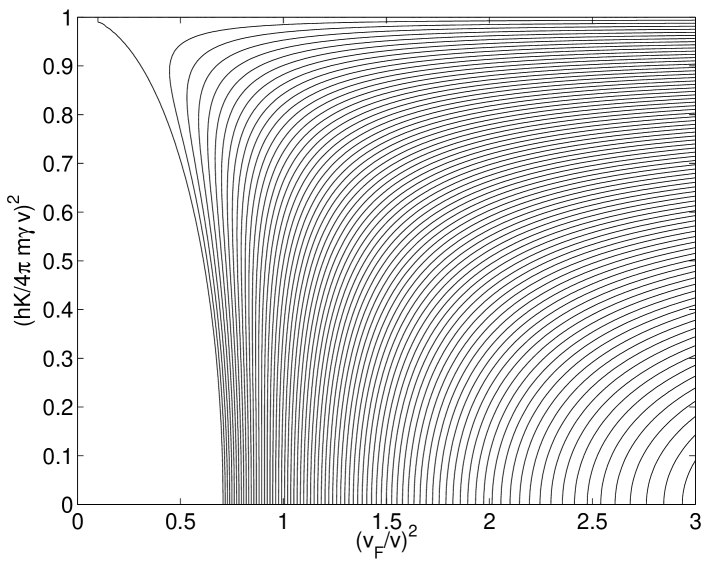
Figure 1: A contour plot of the values of $({\mathnormal{\Gamma}}/Kv)^{2}$, when $\varepsilon=0$, for which the instability occurs. The function $({\mathnormal{\Gamma}}/Kv)^{2}$ is constant along the contours, and plotted in terms of the variables $(v_{F}/v)^{2}$ and $(h/2vm\gamma\ell)^{2}$. Outside the contours ${\mathnormal{\Gamma}}^{2}<0$.

+

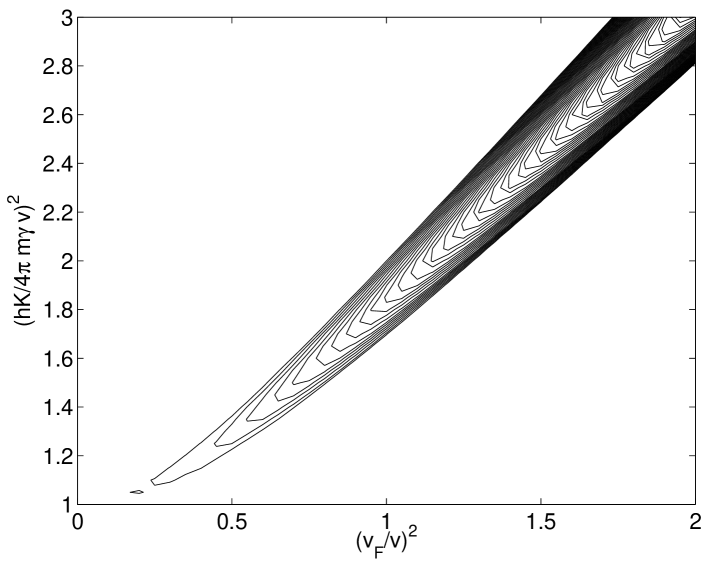
Figure 2: The same plot as in Fig. 1, but for $\varepsilon=2$.

3.2 Partial incoherence and thermal effects

Partial incoherence can in general lead to lower growth rate, similar to inverse Landau damping. As an example of the results of stochastic effects, e.g. thermal fluctuations, we look at the following example. Let the indeterminacy of the wave function manifest itself in a random phase $\varphi(x)$ of the background wave function, with the width $\Delta p$ defined according to $\langle\mathrm{e}^{-i\varphi(x+y/2)}\mathrm{e}^{i\varphi(x-y/2)}\rangle=\mathrm{e}^{-\Delta p|y|/\hbar}$. Due to this random spread, the modulational instability will be damped, as will be shown below. The Wigner function corresponding to the random phase assumption is given by the Lorentz distribution

$$f_{0}(p)=\frac{n_{0}}{\pi}\frac{\Delta p}{(p-p_{0})^{2}+\Delta p^{2}}.$$ (27)

With this, we obtain Eq. (24) with ${\mathnormal{\Gamma}}\rightarrow{\mathnormal{\Gamma}}_{D}+\Delta pK/m\gamma$, where ${\mathnormal{\Gamma}}_{D}$ is the reduced growth rate. Thus, we see that the broadening tends to suppress the growth. Moreover, a positive growth rate ${\mathnormal{\Gamma}}_{D}$ requires

$$\frac{2v\Delta p}{\hbar{\mathnormal{\Gamma}}}<\frac{\ell}{\ell_{0}},$$ (28)

where ${\mathnormal{\Gamma}}$ is given by Eq. (24). Hence, the general property of a spread in momentum space, here exemplified by a random phase, is to put bounds on the modulational instability length scale $\ell$.

Incoherent effects among the neutrinos and anti-neutrinos can also be approached for a background obeying Fermi–Dirac statistics, i.e.

$$f_{0\pm}(p)=\frac{cn_{0}}{\ln(4)k_{B}T_{\pm}}\left[1+\exp\left(\frac{c|p|}{k_{B}T_{\pm}}\right)\right]^{-1},$$ (29)

where we set $M=N=1$, and assume $n_{0}=\bar{n}_{0}$. Here, we have neglected the mass of the neutrinos (which will give us the correct result to lowest order). We will for simplicity assume that $T_{\pm}=T$, so that the dispersion relation (19) takes the form

$$1 = -\frac{4\sqrt{2}\,cG_{F}n_{0}}{\ln(4)\hbar k_{B}T}\int_{-\infty}^{\infty}\,dp\,({\mathnormal{\Omega}}-pK/m\gamma)^{-1}\left[\left(1+\exp(c|p+\hbar K/2|/k_{B}T)\right)^{-1}\right.$$ (30)

$$\qquad\qquad\qquad\left.+\left(1+\exp(c|p-\hbar K/2|/k_{B}T)\right)^{-1}\right].$$

The dispersion relation (30) cannot be solved analytically, but it can be expressed according to

$$1 = -Q\left[\mathrm{P}(I({\mathnormal{\Omega}}_{n},K_{n}))+i\pi g({\mathnormal{\Omega}}_{n},K_{n})\right],$$ (31)

where $\mathrm{P}(I({\mathnormal{\Omega}}_{n},K_{n}))$ is the principal value of the integral

$$I=\int_{0}^{\infty}dx\,(1+\e^{x})^{-1}\left[\frac{{\mathnormal{\Omega}}_{n}+K_{n}^{2}}{({\mathnormal{\Omega}}_{n}+K_{n}^{2})^{2}-K_{n}^{2}x^{2}}+\frac{{\mathnormal{\Omega}}_{n}-K_{n}^{2}}{({\mathnormal{\Omega}}_{n}-K_{n}^{2})^{2}-K_{n}^{2}x^{2}}\right],$$ (32)

and $g=g_{+}+g_{-}$, where

$$g_{\pm}({\mathnormal{\Omega}}_{n},K_{n})=\frac{{\mathnormal{\Omega}}_{n}\pm K_{n}^{2}}{1+\exp(|{\mathnormal{\Omega}}_{n}\pm K_{n}^{2}|/\sqrt{2}K_{n})},$$ (33)

$Q\equiv(4/\ln 4)(2\sqrt{2}\,G_{F}n_{0}/k_{B}T)(m\gamma c^{2}/k_{B}T)$, and we have introduced the dimensionless variables ${\mathnormal{\Omega}}_{n}\equiv(\hbar m\gamma c^{2}/(k_{B}T)^{2}){\mathnormal{\Omega}}$ and $K_{n}\equiv(\hbar c/\sqrt{2}\,k_{B}T)K$. The constant $Q$ gives the ratio of the potential energy contribution of the background and the individual neutrino energy to the thermal energy of the background. Furthermore, $m\gamma c^{2}\simeq k_{B}T$, thus simplifying the expression for $Q$. The contributions from real and imaginary parts to the dispersion relation are plotted in Figs. 3 and 4, respectively. Note that for very short length scales, i.e. large $K$, the quantity ${\mathnormal{\Omega}}_{n}-K_{n}^{2}$ becomes negative, and the imaginary part in Eq. (31) change sign, something which will not show using the long wavelength limit equation (14). This “quantum” behaviour can in principle lead to growth instead of damping of the perturbations (see Ref. [25] for a general discussion of this behaviour). We can obtain a quantitative measure of the growth rate as follows. For any fixed $K_{n0}$, the dimensionless growth rate ${\mathnormal{\Gamma}}_{n}=-i\,\mathrm{Im}\,{\mathnormal{\Omega}}_{n}$ may be expressed as, denoting the value at ${\mathnormal{\Omega}}_{n0}$ by $0$,

$${\mathnormal{\Gamma}}_{n}=\pi\frac{\left(Q^{-1}+\mathrm{P}(I_{0})\right)\,(\partial g/\partial{\mathnormal{\Omega}}_{n0})-g_{0}(\partial\mathrm{P}(I)/\partial{\mathnormal{\Omega}}_{n0})}{\pi^{2}\left(\partial g/\partial{\mathnormal{\Omega}}_{n0}\right)^{2}+\left(\partial\mathrm{P}(I)/\partial{\mathnormal{\Omega}}_{n0}\right)^{2}}$$ (34)

to first order around $({\mathnormal{\Omega}}_{n0},K_{n0})$. Thus, ${\mathnormal{\Gamma}}_{n}>0$ if $\left(Q^{-1}+\mathrm{P}(I_{0})\right)\,(\partial\ln g/\partial{\mathnormal{\Omega}}_{n0})>\partial\mathrm{P}(I)/\partial{\mathnormal{\Omega}}_{n0}$. Moreover, using values given in Sec. 4, one can show that $Q^{-1}\simeq 3\times 10^{9}$. Thus, over a wide range of $({\mathnormal{\Omega}}_{n},K_{n})$, $Q^{-1}$ dominates the contribution to the growth rate, and a positive growth rate is implied as long as $\partial g/\partial{\mathnormal{\Omega}}_{n0}>0$.

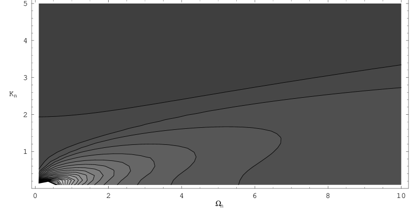
Figure 3: A contour plot of the Cauchy principal value $\mathrm{P}(I({\mathnormal{\Omega}}_{n},K_{n}))$ as a function of the dimensionless variables ${\mathnormal{\Omega}}_{n}$ and $K_{n}$. We note that $\mathrm{P}(I({\mathnormal{\Omega}}_{n},K_{n}))\geq 0$, being largest for small ${\mathnormal{\Omega}}_{n}$ and $K_{n}$, and approaching zero at infinity. The uppermost contour has $\mathrm{P}(I({\mathnormal{\Omega}}_{n},K_{n}))=0$.

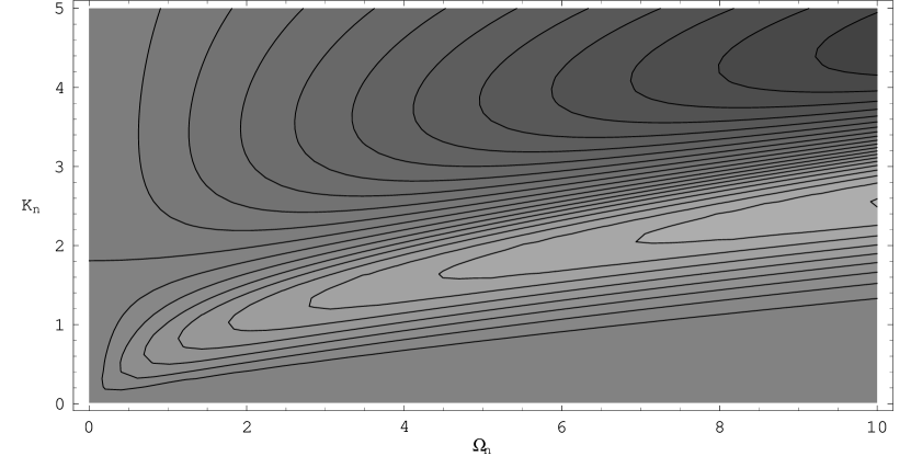
Figure 4: A contour plot of the contribution $g({\mathnormal{\Omega}}_{n},K_{n})$ of the poles to the integral (30) as a function of the dimensionless variables ${\mathnormal{\Omega}}_{n}$ and $K_{n}$. The darker areas represent negative values, the lighter positive values, and $g$ is zero on the contour emanating from $({\mathnormal{\Omega}}_{n},K_{n})=(0,1.8)$.

4 Applications

As a model for hot dark matter, massive neutrinos have for some time been one of the prime candidates, but as such they have faced the problem of the scale of the inhomogeneities they can support. Due to the conservation of phase-space density, the Tremaine–Gunn limit constrains the neutrino mass for isothermal spheres of a given size. For dwarf galaxies, for which there are ample evidence of dark matter [26], the necessary mass of the neutrino is uncomfortably large [4, 27]. On the other hand, as pointed out by Raffelt & Silk [5], interacting dark matter can in principle change this picture. Here we see from Eq. (26) that as the neutrino momentum increases, the typical length scale $\ell$ of the inhomogeneity that can be supported by the modulational instability decreases. From the definition of $\ell_{0}$, we note that as $v$ tends to $c$, $\ell_{0}\rightarrow 0$, and due to Eq. (26) the allowed scale of inhomogeneity becomes squeezed between two small values. On the other hand, if $v\sim v_{F}$ (a condition stating that the neutrino number density must reach extreme values), the upper inhomogeneity scale limit diverges. A minimum requirement for the effect to be of importance is that the instability growth rate is larger than the Hubble parameter $H$. An estimate of the growth rate can be obtained as follows. At the onset of “free streaming” of neutrinos (i.e. their decoupling from matter and radiation) at $z\sim 10^{10}$, the neutrino number density can be estimated as $n_{0}\simeq 2.1\times 10^{38}\,\mathrm{m}^{-3}$ (see, e.g. [28]). Furthermore, we assume that the neutrino mass is in the range $m\sim 1\,\mathrm{eV}$, and find $v_{F}\simeq 2.1\times 10^{6}\gamma^{-1/2}\,\mathrm{m}/\mathrm{s}$. The temperature of the neutrinos, given by $T_{\nu}=(4/11)^{1/3}T_{0}(1+z)$ ($T_{0}$ being the present day CMB temperature) [28], at neutrino decoupling is $T_{\nu}\simeq 2\times 10^{10}\,\mathrm{K}$. Thus, the thermal energy is roughly five orders of magnitude greater than the assumed rest mass of the neutrino, and in this sense the neutrinos can be well approximated as ultra-relativistic. In this case, using values of $(\hbar K/2m\gamma v_{F})^{2}$ in the middle range of the inequality (25), Eq. (24) gives ${\mathnormal{\Gamma}}\simeq 2\sqrt{2}G_{F}n_{0}/\hbar\sim 16\times 10^{10}\,\mathrm{s}^{-1}$ for the values specified above. Assuming a critical density for the Universe, the Hubble time becomes $H^{-1}\simeq H_{0}^{-1}(1+z)^{-3/2}\sim 5\times 10^{2}\,\mathrm{s}$ at a redshift $10^{10}$, and thus ${\mathnormal{\Gamma}}/H\gg 1$.

Although the two-stream instability may seem contrived as a cosmological application, the important issue displayed by this example is the non-gravitational growth of inhomogeneities, given a small perturbation of a homogeneous, although anisotropic, background. The fact that the growth rate exceeds the inverse of the Hubble time by many orders of magnitude makes it clear that the mechanism may be of some importance. Moreover, the analogous estimate for the Fermi–Dirac background, although done in a simplistic manner, indicates that the growth of the large $K$ perturbations may be of importance. Note that this effect is a result of the use of the full Wigner–Moyal system, as compared to the Vlasov system (14), where these short wavelength effects are manifestly neglected. Furthermore, it could also be of interest to use the current formalism as a tool to investigate neutrino interactions within supernovæ, where the two-stream instability scenario may occur as a more natural ingredient than perhaps within cosmology.

5 Conclusion

In conclusion, we have considered the nonlinear coupling between neutrinos and anti-neutrinos in a dense plasma. It is found that their interactions are governed by a system of Wigner-Moyal equations, which admit a modulational instability of the neutrino/antineutrino beams against large scale (in comparison with the neutrino wavelength) density fluctuations. Physically, instability arises because interpenetrating neutrino and antineutrino beams are like quasiparticles, carrying free energy which can be coupled to inhomogeneities due to a resonant quasiparticle-wave interaction that is similar to a Cherenkov interaction. Nonlinearly excited density fluctuations can be associated with the background inhomogeneity of the early Universe, and possibly counteract the free streaming smoothing of the small scale primordial fluctuations, thus making massive neutrinos plausible as a candidate for hot dark matter.

References

- [1] Q. R. Ahmad et al., Phys. Rev. Lett. 89 011301 (2002).
- [2] A. D. Dolgov, Phys. Rep. 370 333 (2002).
- [3] Y. Sofue and V. C. Rubin, Ann. Rev. Astron. Astrophys. 39 137 (2001).
- [4] S. Tremaine and J. E. Gunn, Phys. Rev. Lett. 42 407 (1979).
- [5] G. G. Raffelt and J. Silk, Phys. Lett. B 192 65 (1987)
- [6] F. Atrio–Barandela and S. Davidson, Phys. Rev. D 55 5886 (1997).
- [7] Y. Fukuda et al., Phys. Rev. Lett. 81 1562 (1998); Y. Fukuda et al., Phys. Lett. B 436 33 (1998); Y. Fukuda et al., Phys. Rev. Lett. 82 1810 (1999).
- [8] O. Elgaroy et al., Phys. Rev. Lett. 89 061301 (2002).
- [9] S. Hannestad, Phys. Rev. D 66 125011 (2002); K.N. Abazajian and S. Dodelson, Phys. Rev. Lett. 91 041301 (2003).
- [10] T. K. Kuo and J. Pantaleone, Rev. Mod. Phys. 61 937 (1989).
- [11] L. O. Silva et al., Astrophys. J. 127 481 (2000).
- [12] H. A. Weldon, Phys. Rev. D 26 2789 (1982).
- [13] D. Nötzhold and G. Raffelt, Nucl. Phys. B 307 924 (1988).
- [14] H. Nunokawa et al., Nucl. Phys. B 501 17 (1997).
- [15] G. G. Raffelt, Stars as Laboratories for Fundamental Physics (University of Chicago Press, Chicago, 1996).
- [16] N. L. Tsintsadze et al., Phys. Plasmas 5 3512 (1998); P. K. Shukla et al., Phys. Plasmas 9 3625 (2002).
- [17] V. I. Karpman, Nonlinear Waves in Dispersive Media (Pergamon Press, Oxford, 1975).
- [18] A. Hasegawa, Plasma Instabilities and Nonlinear Effects (Springer-Verlag, Berlin, 1975).
- [19] M. Marklund, P.K. Shukla and L. Stenflo, submitted.
- [20] J. Pantaleone, Phys. Lett. B 342 250 (1995).
- [21] E. P. Wigner, Phys. Rev. 40 749 (1932); J. E. Moyal, Proc. Cambridge Philos. Soc. 45 99 (1949); V. B. Semikoz, Physica A 142 157 (1987).
- [22] B. Hall et al., Phys. Rev. E 65 035602 (2002).
- [23] D. Anderson et al., Phys. Rev. E 65 046417 (2002).
- [24] J.L. Synge, The Relativistic Gas (North Holland, Amsterdam, 1957).
- [25] D. Anderson, L. Helczynski, M. Lisak and V. Semenov, submitted (2003).
- [26] B. Carr, Ann. Rev. Astr. Astrophys. 32 531 (1994).
- [27] Ya. B. Zel’dovich and R. A. Syunyaev, Sov. Astron. Lett. 6 249 (1980); A. G. Doroshkevich et al., Sov. Astron. Lett. 6 252 (1980); A. G. Doroshkevich et al., Sov. Astron. Lett. 6 257 (1980); P. J. E. Peebles, Astroph. J. 258 415 (1982); S. D. M. White, C. S. Frenk and M. Davis, Astrophys. J. Lett. 274 L1 (1983); G. G. Raffelt, New Astronomy Reviews 46 699 (2002).
- [28] P. J. E. Peebles, Principles of Physical Cosmology (Princeton University Press, Princeton, 1993).