X-ray Modeling of Very Young Early Type Stars in the Orion Trapezium: Signatures of Magnetically Confined Plasmas and Evolutionary Implications

Abstract

The Orion Trapezium is one of the youngest and closest star forming regions within our Galaxy. With a dynamic age of $\sim 3\times 10^{5}$ yr it harbors a number of very young hot stars, which likely are on the zero-age main sequence (ZAMS). We analyzed high resolution X-ray spectra in the wavelength range of 1.5 – 25 Å  of three of its X-ray brightest members ($\Theta^{1}$ Ori A, C and E) obtained with the High Energy Transmission Grating Spectrometer (HETGS) on-board the Chandra X-ray Observatory. We measured X-ray emission lines, calculated differential emission measure distributions (DEMs), and fitted broad-band models to the spectra. The spectra from all three stars are very rich in emission lines, specifically from highly ionized Fe which includes emission from Fe XVII to Fe XXV ions. A complete line list is included. This is a mere effect of high temperatures rather than an overabundance of Fe, which in fact turns out to be underabundant in all three Trapezium members. Similarly there is a significant underabundance in Ne and O as well, whereas Mg, Si, S, Ar, and Ca appear close to solar. The DEM derived from over 80 emission lines in the spectrum of $\Theta^{1}$ Ori C indicates three peaks located at 7.9 MK, 25 MK, and 66 MK. The emission measure varies over the 15.4 day wind period of the star. For the two phases observed, the low temperature emission remains stable, while the high temperature emission shows significant differences. The line widths seem to show a similar bifurcation, where we resolve some of the soft X-ray lines with velocities up to 850 km s^-1 (all widths are stated as HWHM), whereas the bulk of the lines remain unresolved with a confidence limit of 110 km s^-1. The broad band spectra of the other two stars can be fitted with several collisionally ionized plasma model components within a temperature range of 4.3 – 46.8 MK for $\Theta^{1}$ Ori E and 4.8 – 42.7 MK for $\Theta^{1}$ Ori A. The high temperature emissivity contributes over 70$\%$ to the total X-ray flux. None of the lines are resolved for $\Theta^{1}$ Ori A and E with a confidence limit of 160 km s^-1. The influence of the strong UV radiation field on the forbidden line in the He-like triplets allows us to set an upper limit on distance of the line emitting region from the photosphere. The bulk of the X-ray emission cannot be produced by shock instabilities in a radiation driven wind and are likely the result of magnetic confinement in all three stars. Although confinement models cannot explain all the results, the resemblance of the unresolved lines and the of the DEM with recent observations of active coronae in II Peg and AR Lac during flares is quite obvious. Thus we speculate that the X-ray production mechanism in these stars is similar with the difference that the Orion stars maybe in a state of almost continuous flaring driven by the wind. We clearly rule out major effects due to X-rays from a possible companion. The fact that all three stars appear to be magnetic and are near zero age on the main sequence also raises the issue whether the Orion stars are simply different or whether young massive stars enter the main sequence carrying significant magnetic fields. The ratio log $L_{x}/L_{bol}$ using the ‘wind’ component of the spectrum is -7 for the Trapezium consistent with the expectation from O-stars. This suggests that massive ZAMS stars generate their X-ray luminosities like normal O stars and magnetic confinement provides an additional source of X-rays.

1 Introduction

Since the discovery of X-ray emission from massive early type stars more than two decades ago (Seward et al. 1979, Harnden et al. 1979) it is an ongoing quest to explain its origins and to develop physical models that consistently predict its characteristics. Although to date no definitive models for the production of X-rays in stellar winds exist, it is widely established that X-rays are produced by shocks forming from instabilities within a radiatively driven wind (Lucy $\&$ White 1980). This phenomenological model has been revised and expanded throughout the years. Lucy (1982) showed that these shocks can exist well out into the terminal flow overcoming the attenuation problem of the previous model. Owocki, Castor, and Rybicki (1988) extended the model in that they showed that reverse shocks are much stronger than forward shocks in an high velocity gas at low densities, deduced from P Cygni absorption in UV resonance line profiles (Puls et al. 1993, Hillier et al. 1993). These models were able to successfully explain the mass loss from a hot luminous star in the UV domain as well as the soft X-ray spectral temperatures, but to date cannot correctly predict observed X-ray fluxes. For example, Feldmeier, Puls $\&$ Pauldrach (1997) see the possibility of mutual collisions of dense gas shells in the outer wind to produce stronger shocks. Claims that the X-ray emission could originate from coronal gas near the stellar photosphere were soon considered unlikely due to the lack of soft X-ray absorption edges (Cassinelli $\&$ Swank 1983) as well as the absence of coronal emission lines in optical spectra (Nordsieck, Cassinelli, $\&$ Anderson 1981).

That all O and early type B stars are strong stellar X-ray emitters is now a well established fact thanks to relentless observations with Einstein and ROSAT (Pallavicini et al. 1981, Chlebowski et al. 1989, Berghöfer et al. 1994, Cassinelli et al. 1994). Typical X-ray luminosities are of the order of $10^{32}$ erg s^-1 for O-stars and $10^{30.5}$-$10^{31.5}$ erg s^-1 for B-stars (Berghöfer, Schmitt, and Cassinelli 1996), while many low-mass (late type) PMS stars radiate at orders of magnitude lower luminosity and only the peak of their luminosity function reaches $10^{31}$ erg s^-1 (Feigelson and Montmerle 1999). Due to the lack of spectral resolving power, however, many results from Einstein and ROSAT were based on statistical properties of a large sample of Stars (Chlebowski et al. 1989, Berghöfer, Schmitt, and Cassinelli 1996). Among these results were that the X-ray luminosity in early type stars typically scales with the bolometric luminosity with log (L_x/L_bol) = -7 and with a few exceptions as high as -5.

In the first very detailed spectral analysis using the ROSAT PSPC, Hillier et al. (1993) fitted spectra of $\zeta$ Pup with NLTE models under the assumptions that the X-rays arise from shocks distributed throughout the wind and that recombination occurs in the outer regions of the stellar wind. The best fits predicted two temperatures of log T(K) $\sim$ 6.2 to 6.7 with shock velocities around 500 km s^-1. Based on this approach, Feldmeier et al. (1997) added the assumption that the X-rays originate from adiabatically expanding cooling zones behind shock fronts and described the spectra with post shock temperature and a volume filling factor. These results were also compared to results from Cohen et al. (1996), who used ROSAT and EUVE data to constrain high-temperature emission models in the analysis of the B-giant, ${}_{p}3.epsilon$ CMa. A continuous temperature distribution was inferred over single or even two temperature models. The result of that comparison remained inconclusive, since both views appeared indistinguishable in the spectra. Despite the success of the wind shock models, several unanswered issues remain from the Einstein , ROSAT , and ASCA era, which seem to be quite in contrast to this model (see also below). One issue concerns the unusually hard X-ray spectra of the B0.2 V star $\tau$ Sco observed with ASCA (Cohen, Cassinelli, $\&$ Waldron 1997), of $\lambda$ Ori (Corcoran et al. 1994), and of ROSAT spectra of stars later than of B2 type (Cohen, Cassinelli, $\&$ MacFarlane 1997).

With the availability of high resolution spectra from Chandra and XMM-Newton the spectral situation became much more complex and confusing. The first published high resolution X-ray spectrum of the Orion Trapezium star $\Theta^{1}$ Ori C showed extreme temperatures and symmetric lines (Schulz et al. 2000 – paper I). These properties are not expected from shocked material near or beyond regions where the wind reached its terminal velocity. Based on a soft X-ray spectrum and symmetric emission lines from $\zeta$ Ori, Waldron and Cassinelli (2001) argued that the emitting plasma originates likely near the photosphere. Highly resolved spectra from $\zeta$ Pup with XMM-Newton (Kahn et al. 2001) and Chandra (Cassinelli et al. 2001) finally showed some expected emission characteristics, i.e. moderate temperatures of 5 to 10 MK, blue shifted and asymmetric lines. Such X-ray line profiles (Ignace 2001, Owocki and Cohen 2001) are significant characteristics of attenuated plasma moving X-ray emitting plasma. Schulz et al. (2001a) and Schulz et al. (2002) report on similar evidence from line profiles in HD 206267 and $\iota$ Ori, respectively.

The fact that the Orion Trapezium star $\Theta^{1}$ Ori C shows such rather strange X-ray characteristics may not come as too much of a surprise, since this star was already known to be of rather peculiar nature (Stahl et al. 1995, Gagne et al. 1997). Babel and Montmerle (1997) proposed an aligned magnetic rotator model. The Orion Trapezium region has always been quite difficult to observe prior to Chandra simply for the fact that its constituent members could never be spatially resolved. The ROSAT HRI (Gagne et al. 1995) provided better spatial resolution, but no spectral information. Yamauchi and Koyama (1993) observed hard X-rays from the Orion Nebula region with GINGA that did not rule out the possibility of 2-3 keV X-rays from $\Theta^{1}$ Ori C, but focused more on possible hard extended emission within the Nebula. This issue was further studied with ASCA (Yamauchi et al. 1996). Highly resolved images and spectra with Chandra could clearly resolve this issue. Schulz et al. 2001 fully resolved the Orion Trapezium in the X-ray band between 0.1 and 10 keV and found no diffuse emission between the Trapezium stars. Furthermore four out of five of the brightest Trapezium stars showed hard X-ray spectra, with $\Theta^{1}$ Ori C being the hottest star showing temperatures of up to 6$\times 10^{7}$ K (paper I).

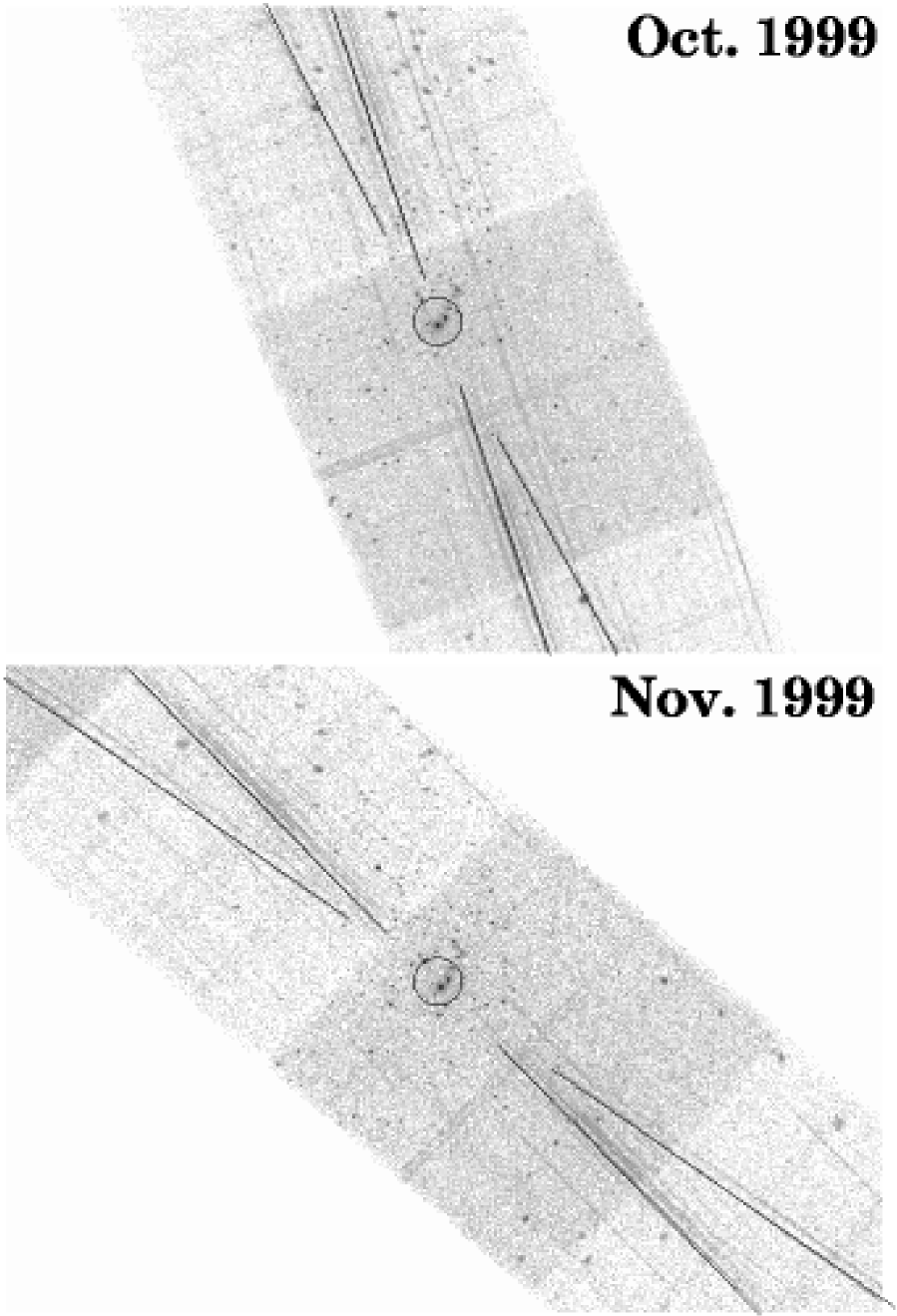
Figure 1: Close-up view of the focal plane image near the zeroth order of the HETGS. The top exposure shows the observation from October 1999, the bottom exposure the one from November 1999, which was performed at a different roll angle. Sky north is up, east is left in both images.

In this paper we further investigate these issues through detailed modeling of High Energy Transmission Grating Spectrometer (HEGTS) spectra from the three X-ray brightest Trapezium stars $\Theta^{1}$ Ori A, C, and E (Schulz et al. 2001). These stars are excellent candidates for such a common study since they are presumably very young; the median age of the Orion Trapezium Cluster is 0.3 Myr (Hillenbrand 1997), they were born at the same time and should have had a quite similar initial chemical conditions. Their spectral types range from O6.5V to B3.

2 Chandra Observations

We accumulate our spectra from two observations in the early phases of the Chandra mission. the first observation was performed on October 31st UT 05:47:21 1999 (OBSID 3) and lasted 50 ks. The second observation was obtained about three weeks later on November 24th UT 05:37:54 1999 (OBSID 4) and lasted 33 ks. For more details of the observations and some of the analysis threads we refer to paper I and Schulz et al. (2001).

2.1 Data Analysis

We re-processed the data using the most recently available calibration and CIAO implementations and produced event lists containing the proper grating dispersion coordinates. The spectral extraction was performed using CIAO tools and we also used custom software for some of the broad band spectral analysis. The modeling of the spectra and its lines was done using ISIS, the emission measure distribution was calculated as in Huenemoerder, Canizares, $\&$ Schulz (2001). As already described in paper I, the Orion Trapezium is embedded in a cluster of fairly bright sources. We thus have to clean each spectrum from contributions of interfering cluster sources, which would imitate lines by coincidence, as well as from dispersed photons of other grating spectra crossing the dispersion track of interest. In our cases of interest the latter effect was entirely eliminated by the energy discrimination by the CCDs. Figure 1 shows the HETGS focal plane view near the zeroth order. In both exposures at the top and bottom part of the figure we encircled the zeroth order positions of the main Trapezium stars. We also highlighted (for illustration purposes only) the tracks of the dispersed spectra for the brightest source $\Theta^{1}$ Ori C.

HEG 1st order spectra of $\Theta^{1}$ Ori C. The top two panels show the +1st and -1st spectrum of the first observation, the bottom two panels the same for the second observation.

The ratio of highly binned (0.5 Å) and smoothed versions of the co-added spectra from the first and second observation, which correspond to a wind-phase difference of approx. 0.45 in $\Theta^{1}$ Ori C.

Many spectral tracks from various Trapezium Cluster stars are detected together with point sources at different off-axis positions which scatter throughout the entire array. One of the differences to the extraction procedure outlined in paper I is that we now have to also extract the spectra of $\Theta^{1}$ Ori A and E, which have a separation of a few arcsec only and are thus more likely to interfere with each other. We make extensive use of the fact that we have observations at two different roll angles, which gives very good separation at least at one roll angle. Besides visual inspection, we also use the fact that we know the relative fluxes of the two sources from the 0th order CCD spectra. In order to minimize the effect of interfering point sources and parallel dispersion tracks of close sources we sometimes narrowed the cross-dispersion selection range. The standard selection range in cross-dispersion engulfs 95$\%$ of the flux and in cases where we narrowed this range we have to re-normalize the fluxes. However we note that by correcting for the expected cross-dispersion profile, we add some systematic errors once we adjust final fluxes. We also correlated detected source point spread functions with the dispersion tracks of the three targets and eliminated the data in the case of a true interference.

2.2 Raw and Exposure Corrected Spectra

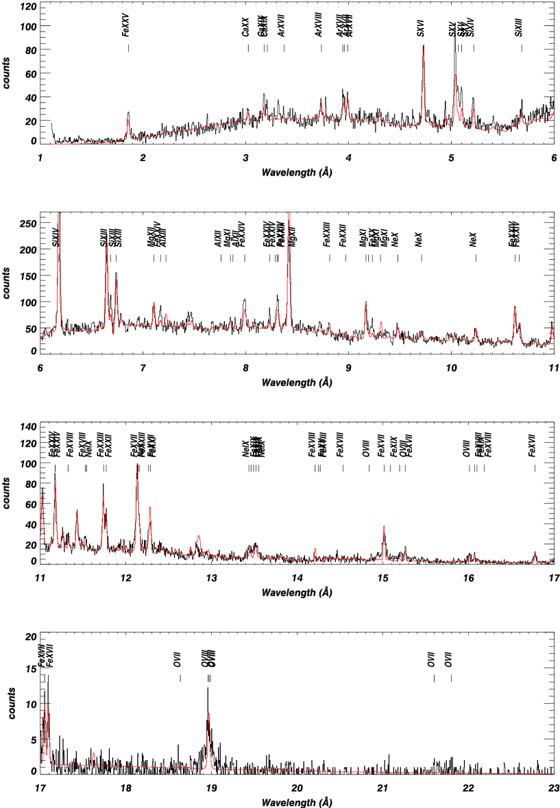
Figure 2: The measured phase averaged count spectrum over the full exposure for $\Theta^{1}$ Ori C. The bins of the spectrum have a value of 0.005 Å. The red line is the approximated phase-averaged plasma model deduced for this spectrum.

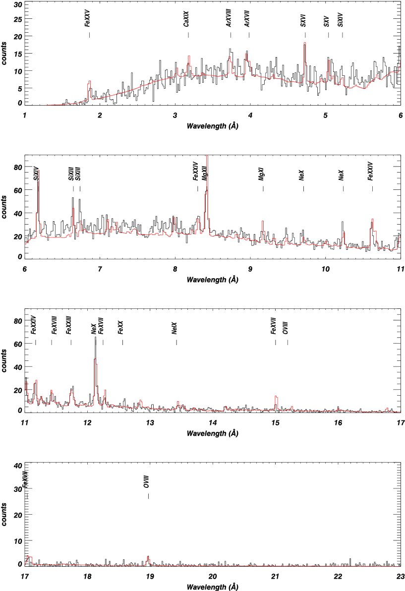
Figure 3: The measured count spectrum for $\Theta^{1}$ Ori E. The red line is the best fit found using a multi temperature APED model

Figure 2 shows the first order HEG spectra of $\Theta^{1}$ Ori C for both observation periods after all cleaning cycles. The weaker appearance of the November 1999 spectra compared to the October 1999 spectra is mostly due the the difference in exposure, but for some lines there may also be variability related to the 15.4 day wind cycle. Here the October observation corresponds to phase 0.82, the November observation to phase 0.37 using the ephemeris from Stahl et al. (1996). In order to investigate this effect we added spectra from the MEG and HEG and divided the exposure corrected flux spectra of the two phases. This spectral ratio is shown in Figure 3. We smoothed and binned the spectra into large (0.5 Å ) bins. The ratio shows that there is a flat part about 38% above unity below 6 Å . The detailed analysis below shows that the changes are due to variable emissivity at high temperatures. The mean (rms) difference across the whole band is about 24$\%$. Schulz et al. (2001) report different fluxes in the zeroth of about 10$\%$, which is consistent given the uncertainties in that observation due to a over $20\%$ pile up fraction.

2.3 Line Widths

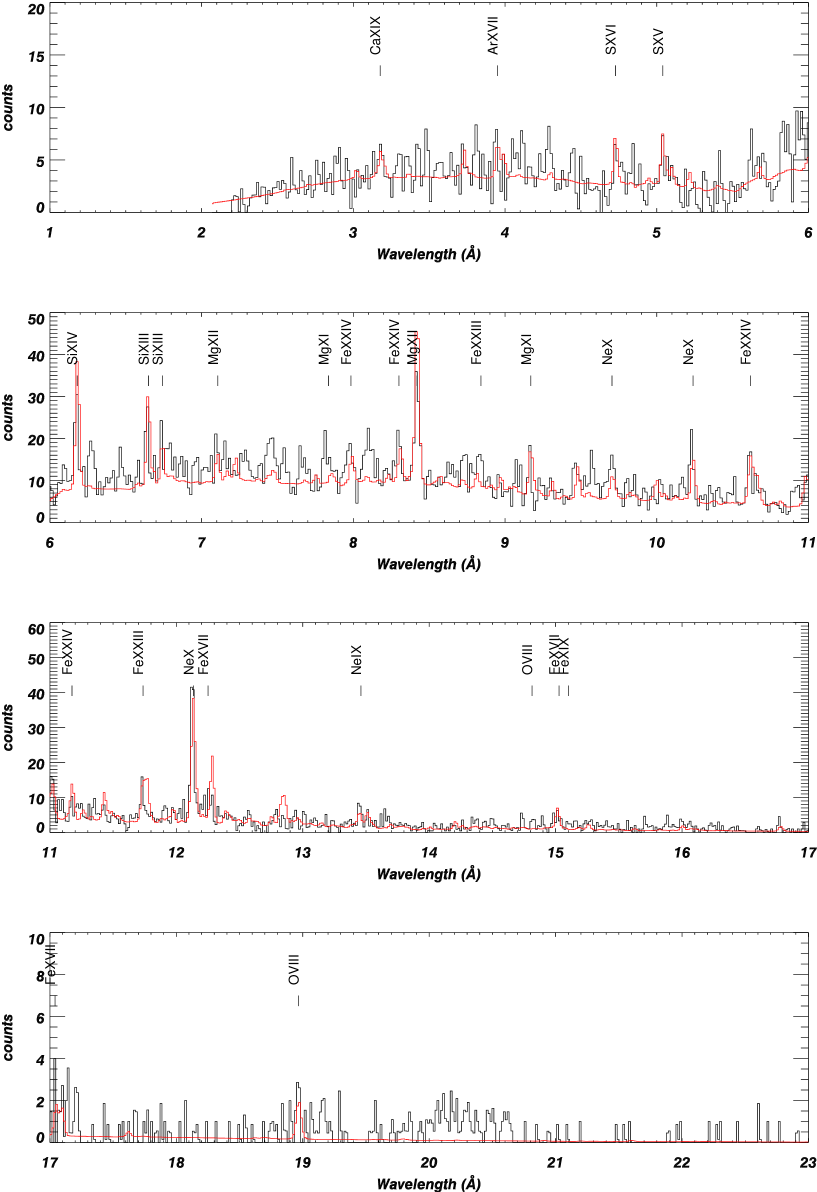
Figure 4: The measured count spectrum for $\Theta^{1}$ Ori A. The red line is the best fit found using a multi temperature APED model

A controversial issue in paper I (see erratum in Schulz et al. 2003) was the analysis of the line widths in the case of $\Theta^{1}$ Ori C. Due to a software error the line width presented in that paper did not properly account for the response of the instrument and, specifically between 10 and 12  Å  underestimated the amount of line blends. Thus the lines appeared wider than they really are. Here we present the analysis that properly includes the instrument response and and takes care of all the line blends. The lines below about 13  Å  clearly appear unresolved. Figure 4 (top) shows lines from three high energy H-like ions, from S XVI, Si XIV, and Mg XII. We chose these these lines because they are most likely not affected by blends. The model used for the line fits is described in section 3.2.2 and it fits not only the local but the overall broad band continuum. Thus the model for all three lines comes from the same fit (Figure 4 bottom). Shown are the co-added spectra and models (red curves). In addition we show a broad stretch from the same model fit between 10.5 and 12  Å  showing many highly ionized and blended Fe states. The model sufficiently describes these blends with no intrinsic broadening. For unresolved lines we can set a 90$\%$ confidence limit of the HWHM of 110 km s^-1 on average based on the statistical properties of the spectrum.

Top: Model fits of three unblended H-like lines. The red curve is the model (as described in section 3.2.2). HEG and MEG data have been co-added, which allows to oversample to profile with spectral bins of 0.003  Å. Bottom: The same model and spectrum in the wavelength range between 10.5 and 12.0  Å. It shows a critical stretch of blended Fe lines. The model includes has zero broadening in the lines.

There is a second population of lines at longer wavelengths which are resolved. The statistical quality for many of them is marginal as in this bandpass the spectrum is effectively absorbed. Figure 5 shows the two brightest resolved lines, one from an Fe XVII ion at 15.01 Å  and the O VIII line at 18.97  Å. The Fe XVII can be fit with a HWHM of 460 km s^-1, the O VIII line with a HWHM of 850 km s^-1. The latter is also the only one we find slightly blueshifted by about 240 km s^-1. In general it is expected to resolve lines better at higher wavelengths since the FWHM is constant with wavelength. However these velocities exceed the confidence limit of 110 km s^-1 for the unresolved lines considerably and this indicates intrinsic broadening for some lower ionization states.

3 Spectral Analysis

We divide the analysis of the $\Theta^{1}$ Ori C spectrum into two parts: we model the broad band spectrum with various temperature components of hot plasmas, and we construct an emission measure distribution from single line emissivities. For the latter we need a large number of significant line fluxes, which we only have available in the case of $\Theta^{1}$ Ori C. For the other hot stars we then compute variations of the broad band plasma model derived from the $\Theta^{1}$ Ori C spectrum.

The two most significant soft lines in the spectrum. The red line shows the model used in Figure 4 with zero line broadening. The green line is a local Gaussian fit to the data. A comparison shows that both lines appear resolved and show significant broadening. The O VIII in the top diagram also appears blue-shifted.

3.1 The Spectral Model

For the spectral modeling we exclusively use the Astrophysical Plasma Emission Code and Database (APEC and APED) described by Smith et al. (2001). The database is available in ISIS and we can compute emissivities for a collisionally ionized equillibrium plasma in terms of temperature, density, and various abundance distributions. In paper I we deduced that these spectra require a range of temperatures. For the model we assume that all emitting plasmas contributing to the spectrum are in collisional ionization equillibrium. This means that a thermal plasma is in a stable ionization state under the coronal approximation. In this approximation it is assumed that the dominant processes are collisional excitation or ionization from the ground state balanced by radiative decay and recombination. Photo-ionization and -excitation as well as collisional ionization from excited states are assumed to be negligible. Note that due to the usually quite strong UV radiation field near the stellar surface this assumption is not quite true and the meta stable forbidden lines in the He-like triplets may be affected. We will discuss the He-like triplets in a separate section.

From over 80 significant lines we calculate a differential emission measure (DEM) distribution for the two phases separately and for the phase averaged spectra. In the other two stars, $\Theta^{1}$ Ori A and E, we lack this large number of lines and cannot calculate such a significant DEM. We therefore approximate the phase averaged DEM of $\Theta^{1}$ Ori C by a few temperature components for which we compute model spectra. We allow as many temperature components as necessary to account for 95$\%$ of the lines (3 $\sigma$) observed. Once adding temperature components does not improve the fit, we allow the abundance distribution to vary against a solar element abundance distribution. A similar procedure was followed to also fit the spectra obtained for $\Theta^{1}$ Ori A and E.

APED model spectra at different temperatures and with solar abundances. The top spectrum was calcula ted at 6 10⁶ K, the middel spectrum corresponds to 1.5 10⁷ K, and the bottom spectrum to 6.0 10⁷ K. The line width was fixed for Doppler velocities of 200 km s^-1.

Top: The distribution of DEMs versus the log of the temperature. The middle curve represents the mean distribution, the top and bottom curve the one $\sigma$ uncertainty envelope from MonteCarlo fitting. Middle: The solid lines represent the upper and lower error envelopes of the DEM from the phase 0.38 spectrum, the dotted lines the ones for the phase 0.76 spectrum. Bottom: The distribution of abundances normalized to solar (which represents 1) versus the ionization potential for various abundant elements for the phase averaged DEM.

Figure 6 demonstrates three typical cases of spectra within the temperature range we found in paper I. All three cases are computed in the low density limit, i.e. for densities below 1$\times 10^{10}$ cm^-3. The spectrum in the top panel has a low temperature of 6 MK. It hardly shows thermal continuum flux, but many lines - mostly from transitions of Fe XVII - in the region around 15 Å . The middle panel shows an intermediate temperature spectrum of 15 MK. We now do not observe Fe transitions below Fe XXII, but very strong Fe XXIV (Li-like) lines in the range between 8 and 12 Å  as well as a faint Fe XXV (He-like) line at 1.85  Å. We also see stronger H- and He-like lines from Si, S, Ar and even Ca. There is already a significant fraction of a thermal continuum. At 60 MK we observe weaker Fe XXIV lines in the 10 to 12 Å  region, but very strong Fe XXV and still strong lines from other high Z elements. Most important is the existence of a strong continuum. This continuum as well as its high energy cut-off value increases with temperature. The value of this cutoff in connection with the Fe XXV emissivity is a sensitive benchmark for the high temperature of the plasma. The continuum also allows measurements of abundances relative to H, since it is dominated by thermal bremsstrahlung. O VIII (Lyman $\alpha$ at 19  Å) is contributing at all temperatures, at higher temperatures the Lyman $\beta$ and $\gamma$ lines become strong as well.

3.2 $\Theta^{1}$ Ori C

We assumed a line-of-sight column density of 1.93$\times 10^{21}$ cm^-2 throughout the entire observation. From the measured color excess of E_B-V = 0.32 (Bolin$\&$Savage 1981) and using the correlation between N_H and E_B-V derived from L_α measurements in hot stars by Savage $\&$ Jenkins 1972 we expect 1.7$\times 10^{21}$ cm^-2; from Spitzer (1978) we expect 1.9$\times 10^{21}$ cm^-2; from Predehl $\&$ Schmitt (1995) we expect 1.4$\times 10^{21}$ cm^-2 for the average interstellar medium (R_v = 3.1) and 2.4$\times 10^{21}$ cm^-2 for dense molecular clouds (R_v = 5.1). From these numbers an additional opacity in the star cannot be concluded.

3.2.1 Emission Measure Distributions

The procedure for the DEM derivation from an X-ray spectrum is described in Huenemoerder, Canizares, $\&$ Schulz (2002). The volume emission measure (VEM) is the volume integral over the product of electron (n_e) and hydrogen (n_h) densities at a given temperature (note: since the emissivity of most emission lines are only weakly dependent on n_e in the expected temperature and density regime, we can as well ignore it). We define a temperature grid of 60 points spaced by 0.05 in log T. The DEM is the derivative of the volume emission measure with respect to log T. It incorporates the emission measure and abundance of many ions and reflects the energy balance of the plasma with respect to temperature.

In Table 1 we show the list of detected lines with measured and predicted line positions and fluxes for the combined spectra. We also, using APED, computed a temperature of maximum emissivity from each ion. The tables are sorted by ion species, which approximately reflects temperature as well.

The first part of Table I shows lines from all Fe ions accepted by the fit with one $\sigma$ confidence errors for the line fluxes. It is specifically remarkable to see a large number of ion states larger than Fe XXII, specifically Fe XXIV, and ion states lower than XIX, specifically Fe XVII. The fractional abundances (i.e. the ratio of integrated flux of a specific ion species over all Fe emission) show a dominance of Fe XXIII to Fe XXV ions ( 0.36) as well as Fe XVII to Fe XIX (0.58), but a significant lack of Fe XX to XXII ions (0.06). The line positions agree well within the expected uncertainties with the positions produced by APED. The second part of Table I shows the list of ions with Z lower than 26. The results are very similar to what we observe for Fe ions, i.e. lines from low and high temperatures dominate the fractional abundances.

Figure 7 (top) shows the DEM versus temperature over a range from 3 to 300 MK. The middle (red) line shows the distribution, the upper and lower lines (green) trace the 90$\%$ uncertainty range. There are clearly three peaks visible at 7.9$\pm$0.2 MK, 26.3$\pm$1.8 MK, and 66.1$\pm$11.2 MK. The emissivity is dominated by plasmas at temperatures higher than 15 MK with a temperature tail that allows the distribution to exceed 100 MK. There is a prominent gap at 7.15 MK that divides the DEM into emission from high and low temperature plasmas. This drop roughly corresponds to the missing emissivities from Fe XX to XXII ions in Table 1. The low temperature peak incorporates most ions from O to Si and Fe XVII to Fe XXII, while the high temperature DEM corresponds to Fe XXIII to Fe XXV, Si to Ca. There is also an incision in the high temperature part of the DEM that roughly corresponds to the weak showing of S XVI and Ca XIX in one of the spectra (see below).

The middle part of Figure 7 show the DEMs for two phases separately. The solid lines show the upper and lower error limits of the DEM for phase 0.82, the dotted lines the same for phase 0.37. There are a few remarkable characteristics. The incision between high and low temperature at 7.15 MK persists in both phases and the low temperature emissivity is similar. The high temperature emissivity shows a significant difference in that the middle peak is much more pronounced in phase 0.82 whereas the high temperature peaks appear unchanged. This means the overall variability in line emissivity is predominately in the Fe XXII and Fe XXIV lines as well as in the Si XIV, where we observe the bulk of the emissivity.

The DEM fit also adjusts abundances (bottom of Figure 7) with respect to solar abundances. Here we find for Mg, Si, S, Ar, Ca ions no significant deviation from solar values. For O we find a factor of 0.2$\pm$0.1, for Ne and Fe a factor of 0.5$\pm$0.1 underabundance. We find this distribution in both observations. Additional uncertainties in these values may stem from uncertainties in the ionization balance (Mazzotta et al. 1998). However we also have to stress the point that once we apply the spectra for each ion fitted in the DEM analysis we find a sufficient fit to the total spectrum (see also below).

The determination of the continuum in the DEM analysis is an iterative process assuming that all continuum contributions come from the same thermal plasma generating the emission lines. Contributions from a non-thermal component critically affect the Fe abundances. A predicted shape of $\propto E^{-1/2}$ of a Compton component (Chen and White 1991) most prominently contributes to the continuum near the Fe XXV line. However the continuum level there is already quite determined by the fits to the Fe XXIV lines and their adjacent continuum levels. We estimate that the contribution cannot be more than about 1$\%$ to the total X-ray flux.

3.2.2 Phase-averaged Plasma Model

Figure 8 shows the phase averaged count spectrum binned by 0.005 Å. MEG and HEG have been added. In this approach we model this spectrum with a few constrained components by approximating the emission measure above. This section in this respect does not produce much new information, but verifies the method used for the fainter stars. However, for reasons of consistency we use the luminosities and fluxes determined in this section for further discussion. We rebin the above DEM into a few coarse intervals and calculate a model component for each DEM interval. We could calculate the model directly from each DEM bin, i.e. from the log T (K) = 0.05 grid. However the idea is to produce a simplified model in good approximation to the DEM. The models were again calculated using the APED database, folded through the spectral response function and were then fit to the measured spectra.

TABLE 1 FE IONS DETECTED IN $\Theta^{1}$ Ori C ion $<$log T$>$ $\lambda_{o}$ $\lambda_{maes}$ flux K Å Å 10^-5 ph s^-1 cm^-2 Fe XXV 7.8 1.860 1.858 7.534$\pm$ 1.225 Fe XXIV 7.4 7.169 7.170 1.341$\pm$ 0.252 Fe XXIV 7.4 7.996 7.989 1.774$\pm$ 0.232 Fe XXIV 7.4 8.316 8.233 0.884$\pm$ 0.200 Fe XXIV 7.4 8.233 8.285 0.248$\pm$ 0.177 Fe XXIV 7.4 8.285 8.304 0.924$\pm$ 0.348 Fe XXIV 7.4 10.619 10.620 5.825$\pm$ 0.585 Fe XXIV 7.4 10.663 10.660 3.453$\pm$ 0.494 Fe XXIV 7.4 11.029 11.032 3.359$\pm$ 1.209 Fe XXIV 7.4 11.176 11.175 7.026$\pm$ 0.718 Fe XXIII 7.2 8.304 8.316 1.484$\pm$ 0.364 Fe XXIII 7.2 8.815 8.816 1.139$\pm$ 0.243 Fe XXIII 7.2 10.981 10.981 3.029$\pm$ 0.456 Fe XXIII 7.2 11.019 11.019 2.592$\pm$ 0.000 Fe XXIII 7.2 11.736 11.739 5.927$\pm$ 0.693 Fe XXIII 7.2 12.161 12.160 3.388$\pm$ 0.950 Fe XXII 7.1 8.975 8.974 0.561$\pm$ 0.224 Fe XXII 7.1 11.770 11.771 4.141$\pm$ 0.602 Fe XXI 7.1 12.284 12.286 4.355$\pm$ 0.908 Fe XX 7.0 9.219 9.194 1.151$\pm$ 0.272 Fe XX 7.0 14.267 14.248 0.614$\pm$ 0.667 Fe XIX 6.9 10.816 10.814 0.862$\pm$ 0.307 Fe XIX 6.9 13.462 13.460 3.366$\pm$ 0.970 Fe XIX 6.9 13.497 13.490 3.536$\pm$ 0.950 Fe XIX 6.9 13.518 13.520 5.639$\pm$ 1.157 Fe XIX 6.9 15.079 15.086 2.156$\pm$ 1.182 Fe XIX 6.9 16.110 16.098 1.637$\pm$ 1.006 Fe XVIII 6.8 11.326 11.324 1.433$\pm$ 0.372 Fe XVIII 6.8 11.527 11.525 1.532$\pm$ 0.521 Fe XVIII 6.8 14.208 14.208 3.472$\pm$ 1.057 Fe XVIII 6.8 14.256 14.268 0.943$\pm$ 0.626 Fe XVIII 6.8 14.534 14.535 1.493$\pm$ 0.658 Fe XVIII 6.8 16.071 16.071 4.501$\pm$ 1.445 Fe XVIII 6.8 16.159 16.184 1.100$\pm$ 0.804 Fe XVII 6.8 10.770 10.764 0.565$\pm$ 0.289 Fe XVII 6.7 12.124 12.129 8.754$\pm$ 1.168 Fe XVII 6.7 12.266 12.265 2.184$\pm$ 0.580 Fe XVII 6.7 15.014 15.014 18.463$\pm$ 2.347 Fe XVII 6.7 15.261 15.261 5.316$\pm$ 1.181 Fe XVII 6.7 16.780 16.775 10.039$\pm$ 2.255 Fe XVII 6.7 17.051 17.051 8.044$\pm$ 2.099 Fe XVII 6.7 17.096 17.095 6.147$\pm$ 1.921

TABLE 1 CONT.: LOWER ($<26$) Z IONS ion $<$log T$>$ $\lambda_{o}$ $\lambda_{maes}$ flux K Å Å 10^-5 ph s^-1 cm^-2 Ca XX 7.8 3.024 3.024 0.602$\pm$ 0.285 Ca XIX 7.5 3.177 3.179 1.206$\pm$ 0.326 Ca XIX 7.5 3.207 3.209 0.752$\pm$ 0.292 Ar XVII 7.4 3.365 3.372 0.303$\pm$ 0.325 Ar XVIII 7.7 3.731 3.735 1.002$\pm$ 0.359 Ar XVII 7.4 3.949 3.943 1.695$\pm$ 0.380 Ar XVII 7.3 3.966 3.960 1.243$\pm$ 0.489 S XVI 7.6 4.733 4.729 5.327$\pm$ 0.619 S XV 7.2 5.039 5.039 5.201$\pm$ 0.710 S XV 7.2 5.067 5.065 1.798$\pm$ 0.486 S XV 7.2 5.102 5.100 2.378$\pm$ 0.541 Si XIV 7.4 5.218 5.217 2.394$\pm$ 0.510 Si XIV 7.4 6.180 6.181 11.662$\pm$ 0.562 Si XIII 7.0 5.681 5.684 0.836$\pm$ 0.276 Si XIII 7.0 6.648 6.648 7.432$\pm$ 0.472 Si XIII 7.0 6.687 6.686 2.515$\pm$ 0.328 Si XIII 7.0 6.740 6.740 3.717$\pm$ 0.342 Al XII 7.0 7.757 7.760 0.595$\pm$ 0.196 Al XII 6.9 7.872 7.874 0.256$\pm$ 0.184 Mg XII 7.2 7.106 7.105 1.554$\pm$ 0.235 Mg XI 6.9 7.850 7.850 0.747$\pm$ 0.206 Mg XII 7.2 8.419 8.420 8.406$\pm$ 0.484 Mg XI 6.8 9.169 9.168 3.085$\pm$ 0.370 Mg XI 6.8 9.231 9.230 1.966$\pm$ 0.314 Mg XI 6.8 9.314 9.310 0.917$\pm$ 0.305 Ne X 7.0 9.481 9.478 1.351$\pm$ 0.271 Ne X 7.0 9.708 9.710 0.889$\pm$ 0.250 Ne X 7.0 10.240 10.240 1.822$\pm$ 0.334 Ne IX 6.6 11.544 11.542 0.595$\pm$ 0.454 Ne X 6.9 12.132 12.144 5.325$\pm$ 1.131 Ne IX 6.6 13.447 13.435 3.804$\pm$ 0.995 Ne IX 6.6 13.550 13.550 3.827$\pm$ 0.962 O VIII 6.7 14.821 14.840 0.930$\pm$ 0.622 O VIII 6.7 15.176 15.195 2.767$\pm$ 0.910 O VIII 6.7 16.006 16.010 3.934$\pm$ 1.200 O VII 6.4 18.627 18.635 4.067$\pm$ 2.007 O VIII 6.7 18.973 18.970 21.143$\pm$ 3.008 O VII 6.3 21.602 21.600 10.230$\pm$ 5.583 O VII 6.3 21.804 21.799 10.451$\pm$ 5.991

TABLE 2 TEMPERATURE COMPONENTS FROM MODEL FITS star comp. log T norm L_x (1-10 keV) $\#$ K erg s^-1 cm^-2 erg s^-1 $\Theta^{1}$ Ori C 1 6.79$\pm$0.06 6.55$\times 10^{-13}$ 7.93$\times 10^{30}$ 2 6.97$\pm$0.07 2.22$\times 10^{-12}$ 2.69$\times 10^{31}$ 3 7.22$\pm$0.07 1.24$\times 10^{-12}$ 1.50$\times 10^{31}$ 4 7.47$\pm$0.08 4.62$\times 10^{-12}$ 5.60$\times 10^{31}$ 5 7.64$\pm$0.06 2.51$\times 10^{-12}$ 3.04$\times 10^{31}$ 6 7.82$\pm$0.07 5.20$\times 10^{-12}$ 6.30$\times 10^{31}$ $\Theta^{1}$ Ori E 1 6.63$\pm$0.08 1.55$\times 10^{-13}$ 1.87$\times 10^{30}$ 2 7.02$\pm$0.08 3.78$\times 10^{-13}$ 4.60$\times 10^{30}$ 3 7.31$\pm$0.07 4.88$\times 10^{-13}$ 5.92$\times 10^{30}$ 4 7.49$\pm$0.06 1.85$\times 10^{-13}$ 2.23$\times 10^{30}$ 5 7.67$\pm$0.06 1.31$\times 10^{-12}$ 1.59$\times 10^{31}$ $\Theta^{1}$ Ori A 1 6.68$\pm$0.09 3.41$\times 10^{-14}$ 4.13$\times 10^{29}$ 2 7.06$\pm$0.08 3.54$\times 10^{-13}$ 4.29$\times 10^{30}$ 3 7.34$\pm$0.08 1.08$\times 10^{-13}$ 1.31$\times 10^{30}$ 4 7.48$\pm$0.07 4.28$\times 10^{-13}$ 5.18$\times 10^{30}$ 5 7.63$\pm$0.07 2.76$\times 10^{-13}$ 3.35$\times 10^{30}$

We fit only one component at a time (keeping the parameters of the other ones fixed) and repeated this step with the other components until the final spectrum meets the criteria below. To sensitively constrain the model we use the DEMs above, which helps us to constrain the relative strengths of the components: the level of the continuum, the position of its high-energy cut-off, the strength of the Fe XXV lines and various temperature dependent line ratios.

Our model reproduces all major properties of the spectrum. There are several small deviations relating to the fact that the model cannot yet reproduce all subtle details. The results are summarized in Table 2. The stated temperature uncertainties are large which is a consequence of the large error envelopes of the DEM in combination with a now very coarse temperature grid. The stated fluxes and luminosities have errors between 5 and 15$\%$. Several key properties in the spectrum are well modeled: the total flux derived from the model and from the exposure corrected data in the range of 1 to 25 Å  agree within 2$\%$, the continuum is well represented and the line ratios agree within 10$\%$.

The final result is overplotted in Figure 8. The thermal flux continuum shows a cut-off around 3.4 Å. In order to get this cut-off we need a high temperature of 66.5 MK. The shallow decline of the continuum below the cut-off requires stronger intermediate temperature components (43.8 and 29.5 MK), which are constrained by by line ratios of Si, S, and Fe lines as well as the fact that the sum of the Fe XXV line fluxes of these two high temperature components need to match the observed line flux. These three components account for almost all of the continuum providing 75$\%$ of the star’s X-ray luminosity. The low temperature components at 6.1, 9.3 and 16.5 MK produce many lines between 9 and 20 Å  but account only for a fraction of the total luminosity. In fact, if the star did not have hot components, it would be faint. From Table 2 the X-ray luminosity accounting for the low temperature DEM component only is 3.5$\times 10^{31}$ erg s^-1 . Using the bolometric luminosity as listed by Berghöfer, Schmitt, and Cassinelli (1996) we find -7.2 for the low temperature log $L_{x}/L_{bol}$. More than 85$\%$ of the luminosity is radiated by plasmas with temperatures higher than 1.5$\times 10^{7}$ K, and 75$\%$ from temperatures higher than 3$\times 10^{7}$ K. This is consistent with the results from the zero order CCD spectra (Schulz et al. 2001). The abundances had to be adjusted during the fit as well and the result is similar to the distribution observed in the DEM analysis.

The He-like triplets from S (top), Si (middle), and Mg (bottom) from the spectrum in figure 8. The model here has been optimized such for each triplet that it fits the recombination line.

3.2.3 Optical depths, Formation Radii and Densities

Line ratios may be used to place limits on optical depths, line formation radii and densities. Schmelz, Saba, and Strong (1992) suggested that the Fe XVII (upper-level $2p^{5}3d^{1}P_{1}$) line at 15.01  Å could be used as a measure for resonant scattering (and thus density) in the emitting plasma. Specifically the ratio to its Fe XVII resonance line neighbor at 15.26 Å ($2p^{6}~{}~{}^{1}S_{0}-2p^{5}3d^{3}D_{1}$) is of interest (see also Waljeski et al. 1994, Brickhouse et al. 2000 and a discussion in Huenemoerder, Canizares, and Schulz 2001). From the APED database we deduce a theoretical ratio of 3.57 for the optically thin limit. The measured ratio in the spectrum is 3.47$\pm$1.21 and thus despite the large error bar indicates agreement with a low density plasma. The formation radius of this line can be estimated from its line width. This line was indeed resolved with a HWHM of 460 km s^-1. The standard law of velocity for the acceleration zone of the wind $v(r)=v_{\infty}(1-r_{star}/r)^{\beta}$ (Lamers $\&$ Cassinelli 1999) with the index $\beta$ =0.88 and a terminal velocity of 1000 km s^-1 would then locate the line emitting region to slightly more than half a stellar radius from the photosphere.

Another line that was resolved was the O VIII line at 18.97  Å. Its HWHM corresponds to velocity of 850 km s^-1, which would place the emitting region almost near the terminal velocity of the wind at about 7 seven stellar radii from the photosphere. In contrast, the line width limit of 110 km s^-1 would place the emitting radius of all the other (non He-like) lines to within 10$\%$ of a stellar radius above the photosphere (see also Cohen et al. 2002 for $\tau$ Sco). Whether there should be an asymmetry of the line due to occultation seems irrelevant since we do not resolve most of the lines.

The forbidden lines in the He-like triplets are meta-stable and their ratio with the corresponding intercombination lines is density sensitive above some ion-dependent theshold. Figure 9 shows the observed He-like triplets from S XV, Si XIII, and Mg XI. The model fits for these triplets have been optimized for each element to specifically fit the resonance line. One of the most striking effects seen in the triplets from O VII (very faint), Ne IX, and Mg XI (Figure 9, bottom) is that the forbidden line is not observed, while it still appears quite prominent in Si XIII and S XV (Figure 9 middle and top). Although the forbidden transition in the Si XIII triplet is blended with the Lyman $\gamma$ line of Mg XII, based on the flux observed in the Mg XII Lyman $\alpha$ line, the Lyman $\gamma$ contribution cannot be more than 5$\%$. However we observe a forbidden line flux comparable to the expectation of the model. We observe a similar picture in S XV (which is not blended), however the f/i ratio here is not sensitive to densities lower than $10^{14}$ cm^-3.

All the triplets are subject to UV excitation and it has been shown by Kahn et al. (2001) (see also Blumenthal, Drake, and Tucker 1972) in the example of $\zeta$ Pup that the low $f/i$ ratios in line driven wind plasmas are not likely an effect of collisional excitation in high density plasmas, but rather are due to the destruction of the forbidden line by the large UV flux at the corresponding excitation wavelengths. Waldron and Cassinelli (2001), Cassinelli et al. (2001) and Miller et al. (2002) use model UV fluxes (e.g. Chavez, Stalio, and Holberg 1995) to estimate radial constraints on the X-ray emitting plasma. Such an analysis in the case of $\Theta^{1}$ Ori C is highly delicate. One critical item is the modeling of the actual UV flux between $\sim$ 900 and 1500  Å, which provides the source for the photoexcitation in Si XIII, and Mg XI. We checked the ratio of the UV spectra of $\Theta^{1}$ Ori C and $\zeta$ Pup using Copernicus data (Snow $\&$ Jenkins 1977) and after correcting for the different stellar parameters (19 $R_{\odot}$ , 42500 K, $E_{B-V}$ = 0.07 for $\zeta$ Pup; 8 $R_{\odot}$ , 39000 K, $E_{B-V}$ = 0.35 for $\Theta^{1}$ Ori C; Pauldrach et al. 1994, Howard $\&$ Prinja 1989, Berghöfer, Schmitt, and Cassinelli 1996) we could not quite reconcile the model with the data in a sense that the UV flux in $\Theta^{1}$ Ori C seems lower than the model. A proper correction for extinction is certainly critical.

Effectively there no obvious reason why the UV field should be weaker than one would expect from blackbody model atmospheres (MacFarlane et al. 1993, Chavez, Stalio, and Holmberg 1995). In this respect we estimated the formation radius by assuming a blackbody spectrum of 39000 K for the radiation field for an O7V star (Howard $\&$ Prinja 1989) as an upper limit. The surface temperature of $\Theta^{1}$ Ori C is also a source of uncertainty, as $\Theta^{1}$ Ori C is classified somewhere between O6 and O7.5, sometimes even as O4. In case of the latter the result can differ by over 60$\%$. We calculated the photoionization (PE) rates using the recipe provided by Kahn et al. (2001, see also Mewe $\&$ Schrijver 1978) and obtained 2 ${}^{3}S-1^{1}S$ decay rates from Drake (1971). In Mg XI the forbidden line can be only marginally detected above the 1 $\sigma$ error of the continuum and here we consider the radius where the PE rate is of the order of the decay rate as critical. The $f/i$ ratios in Si and S are, though reduced from the one expected from the atomic data in the optically thin limit, significantly larger. Here we have to assume that the formation radius is farther away from the stars surface and the PE rate is correspondingly smaller. Thus for Mg we find an upper limit to the formation radius of 4.2 stellar radii, for Si 2.0 stellar radii and 1.3 stellar radii for S.

On the other hand it should be mentioned that in the case of zero UV flux the $f/i$ ratio of the triplets can also be used as density diagnostics. We then obtain densities of $<4\pm 2\times 10^{13}$ cm^-3 for Mg and $<9\pm 8\times 10^{13}$ cm^-3 for Si, repeating the result stated in paper I.

3.3 $\Theta^{1}$ Ori E and A

The next two X-ray brightest stars in the Trapezium are stars A and E with X-ray fluxes of 1.3 to 2.5$\times 10^{-12}$ erg cm^-2 s^-1 corresponding to luminosities of 2 to 4$\times 10^{31}$ erg s^-1 , respectively (Schulz et al. 2001). These fluxes are an order of magnitude fainter than $\Theta^{1}$ Ori C, which is likely due to their B spectral types (Cassinelli et al. 1994). In this respect the HETGS spectra are less brilliant, however in both spectra we are still able to detect quite a number of emission lines and strong continua. This at least allows us to sufficiently constrain our multicomponent model. Table 3 shows the characteristics of the brightest lines for both stars. These line properties are very similar to the characteristics exhibited by $\Theta^{1}$ Ori C. This is specifically noteworthy for the Fe XXIV transitions. The lines appear unresolved in both stars and we can set a HWHM confidence limit of 160 km s^-1. In general we observe the same most remarkable features: the strong continuum and very narrow and symmetric lines.

Figures 10 and 11 show the count spectra of the two stars binned to 0.015 Å. The red solid lines are the final model spectra. We fitted these spectra following the procedure described in section 3.2.2. The result for $\Theta^{1}$ Ori E is shown in the middle part, for $\Theta^{1}$ Ori A in the bottom part of Table 3. Both spectra accepted 5 components including a quite marginal low temperature component. The four higher temperature components seem similar to components 2-5 in $\Theta^{1}$ Ori C, with the one for the very high temperature missing. In this respect we observe a similar bifurcation in emissivity in stars A and E, which includes low temperature emissivity below at or below 10⁷ K and strong emissivity that has temperatures significantly higher than 10⁷ K. In the case of $\Theta^{1}$ Ori E roughly 80$\%$ and for $\Theta^{1}$ Ori A 70$\%$ of the luminosity appears at temperatures higher than 1.5$\times 10^{7}$ K. Over 50$\%$ of the luminosity originates from emitting plasmas showing temperatures higher than 3$\times 10^{7}$ K. Thus if we again only count the flux of the low temperature component as the one form the unconfined wind, the ratio $L_{x}^{wind}/L_{bol}$ for these two sources are similar the the one for $\Theta^{1}$ Ori C and thus consistent with normal O-stars. The fit abundances are also similar to values for $\Theta^{1}$ Ori C, except that the Ne lines are stronger, and we do not detect a deviation from solar values.

Most He-like triplet are too weak to perform a meaningful analysis except for Si XIII, where in the case of star E (Figure 10, 6.74 Å) we observe a forbidden line that is almost as strong as the resonance line. In star A it is not as strong but clearly detectable. In both cases we do not detect an intercombination line and by setting a limit to the line using the 1 $\sigma$ error of the continuum we can only get rough estimate of the $f/i$ ratio. We nevertheless we can put some limits on the formation radius of Si XIII. In the optically thin limit without photoexcitation we expect 2.16 for the $f/i$ ratio. For star E we can limit the ratio to 3.43$\pm$1.69, consistent with the then limit and basically no UV destruction. Assuming a B0.5V star with a surface temperature of 23000, we would expect the forbidden line would get completely destroyed within 0.4 stellar radius above the photosphere. Since this is not the case and the line seems to be fully intact, we assume that the 2 ${}^{3}S-1^{1}S$ decay rate entirely dominates the PE rate, which should occur at a distance of 1.4 stellar radii. For star A the ratio is 2.13$\pm$1.33 we can make the same argument assuming a surface temperature of 20000 K (B1V, Strickland 2000). In terms of density, i.e. under the assumption that there is no photoexcitation, the $f/i$ ratios seem to be in compliance with the densities below 10¹³ g cm^-3.

TABLE 3 : IDENTIFIED IONS IN $\Theta^{1}$ Ori A and E ion $\lambda_{o}$ flux ($\Theta^{1}$ Ori A) flux ($\Theta^{1}$ Ori E) Å 10^-6 ph s^-1 cm^-2 10^-6 ph s^-1 cm^-2 Fe XXV 1.861 - 7.182$\pm$ 1.077 Ca XIX 3.198 0.895$\pm$ 0.134 1.481$\pm$ 0.222 Ar XVIII 3.734 - 3.321$\pm$ 0.498 Ar XVII 3.949 0.298$\pm$ 0.045 2.274$\pm$ 0.341 S XVI 4.730 0.840$\pm$ 0.126 5.233$\pm$ 0.785 S XV 5.039 1.097$\pm$ 0.165 2.737$\pm$ 0.411 Si XIV 5.217 - 1.194$\pm$ 0.179 Si XIV 6.183 3.293$\pm$ 0.494 3.935$\pm$ 0.590 Si XIII 6.648 1.731$\pm$ 0.260 2.573$\pm$ 0.386 Si XIII 6.740 1.706$\pm$ 0.256 2.751$\pm$ 0.413 Fe XXIV 7.989 0.676$\pm$ 0.101 - Fe XXIV 8.304 0.676$\pm$ 0.101 1.658$\pm$ 0.249 Mg XII 8.420 2.612$\pm$ 0.392 5.060$\pm$ 0.759 Fe XXIII 8.815 1.363$\pm$ 0.204 - Mg XI 9.169 1.963$\pm$ 0.294 2.495$\pm$ 0.374 Ne X 9.708 0.811$\pm$ 0.122 2.393$\pm$ 0.359 Ne X 10.239 3.078$\pm$ 0.462 3.530$\pm$ 0.530 Fe XXIV 10.619 2.919$\pm$ 0.438 3.508$\pm$ 0.526 Fe XXIII 10.983 - 2.048$\pm$ 0.307 Fe XXIV 11.176 1.013$\pm$ 0.152 4.392$\pm$ 0.659 Fe XXIII 11.736 2.186$\pm$ 0.328 2.875$\pm$ 0.431 Fe XVIII 11.330 - 3.442$\pm$ 0.516 Ne X 12.135 14.589$\pm$ 2.188 16.331$\pm$ 2.450 Fe XVII 12.261 1.558$\pm$ 0.234 0.498$\pm$ 0.075 Fe XX 12.576 - 1.617$\pm$ 0.242 Ne IX 13.445 5.727$\pm$ 0.859 37.722$\pm$ 5.658 Fe XVII 15.014 21.573$\pm$ 3.236 4.164$\pm$ 0.625 Fe XIX 15.079 8.305$\pm$ 1.246 - O VIII 15.176 - 18.360$\pm$ 2.754 Fe XVII 17.051 5.309$\pm$ 0.796 13.059$\pm$ 1.959 O VIII 18.970 0.177$\pm$ 0.027 9.362$\pm$ 1.404

4 Discussion

High resolution X-ray spectra provide new and more powerful diagnostics of the high energy emission from hot star plasmas. These diagnostics involve line identifications, the relation of specific line ratios with physical parameters such as temperature and density, line shapes and shifts as well as full scale plasma models. In paper I we presented a preliminary line list for $\Theta^{1}$ Ori C. For this paper we added one more observation to the analysis for a net exposure of 83 ks. The availability of improved calibration products and models allowed us to refine these results in major areas. For $\Theta^{1}$ Ori C the number of detected lines increased and allowed for better constraints on the plasma modeling specifically for the calculation of the DEM. The DEM analysis of the phase averaged spectrum as well as the fitting of the broad band plasma model showed that the bulk of the X-ray emission comes from plasmas with temperatures above 15 Million K and only a small, well separated part of the emission corresponds to emission of lower than 10 Million K.

There are models related to the standard line-driven wind instability model that are able to allow temperatures in excess of 10 Million K (Feldmeier et al. 1997a, Howk et al. 2000, Runacres$\&$Owocki 2002). However possible high shock velocities near the onset of the wind cannot produce enough volume emissivity to account for the X-ray spectrum. The results also confirm a similar behavior for $\Theta^{1}$ Ori A $\&$ E. This means the bulk of the X-ray emission in the bright Orion Trapezium stars is not compatible with any form of instabilities in a line-driven wind. In fact these stars seem to be of a hybrid nature where only a small fraction of the X-rays are produced in wind shocks, a larger fraction shows a magnetic origin and bears striking similarities to the hard X-ray emission pattern observed in stars with active coronae (Huenemoerder, Canizares, and Schulz 2001, Huenemoerder et al. 2003).

The DEM model allows for a non-thermal continuum component that contributes less than 1$\%$ to the total flux for a power law index of -0.5 as suggested by Chen and White (1991). These authors proposed a non-thermal origin for possible hard X-rays in form of an inverse Compton continuum. This limit corresponds to 4$\times 10^{30}$ erg s^-1 , which is an order of magnitude higher than predicted. Thus we may not really be sensitive to the issue. It is quite clear though that the high energy flux from the Orion Trapezium stars is not due to a possible non-thermal origin.

4.1 Possible Shocked Wind Component

The emissivity peak at log T = 6.9 includes most lines from O to Si and ions below Fe XX. These are the moderate temperature lines we also observe in wind shocks in $\zeta$ Pup and others (Cassinelli et al. 2001, Kahn et al. 2001, Waldron and Cassinelli 2001, Schulz et al. 2001a, Schulz et al. 2002) suggesting a similar origin for this component on $\Theta^{1}$ Ori C. This peak does not change within the two observed phases of the 15.4 day cycle in $\Theta^{1}$ Ori C. Ignace (2001) and Owocki and Cohen (2001) calculated the shape of X-ray line profiles in stellar winds under various conditions.

The fact that most lines in the spectra do not show significant shifts and are unresolved puts limits on these conditions. If the lines were to be produced at large radii in the outer wind, we should observe broad, symmetric, sometimes flat topped lines. Yet for wind shocks, the only way to achieve symmetry is to have almost no attenuation in wind. Given the low mass loss rate of $\sim 4\times 10^{-7}$ $M_{\odot}$ yr^-1 (Howarth $\&$ Prinja 1989) this is quite likely. Some of the X-ray emitting plasma also has to be near the photosphere at the onset of the wind given the unresolved nature of the lines. However it seems that some of the softest lines are indeed resolved and show velocity broadening of up to 850 km s^-1. This is indicative that these lines contributing to the low temperature emissivity peak are due to X-rays from shocks in the outer wind. Would this low temperature emissivity be the only contribution to the X-ray emission, the Orion stars would be quite X-ray faint, but with a log $L_{x}/L_{bol}$ between -7.2 and -7.6, which is near the canonical value for O stars.

4.2 Magnetically Confined Winds

The truth is, however, that log $L_{x}/L_{bol}$ is more of the order of -6.5 for these stars. Since most emissivity appears to originate at temperatures that are incompatible with wind shocks, we have to look for other mechanisms. There are several indications that the enhanced X-ray activity could be triggered by magnetic fields. Gagne et al. (1997) interpreted the strong 15.4 day period in the X-ray and optical emission of $\Theta^{1}$ Ori C reported by Stahl et al. (1996) in terms of the star’s significant magnetic field.

Babel and Montmerle (1997a) proposed a magnetically confined wind shock (MCWS) model based on an oblique magnetic rotator model for $\Theta^{1}$ Ori C. Here the wind is confined by a magnetic dipole field and forced into the magnetic equatorial plane. The observed 15.4 day variability thus is produced by the tilt of the dipole field relative to the rotational axis. The predicted field is of the order of 300 G. Very recent spectrophotometric observations indicate a dipole field of 1.1 kG with an inclination of 42^o with respect to the stars rotational axis (Donati et al. 2002). These values are quite consistent with the temperatures we observe in the spectrum of $\Theta^{1}$ Ori C. This model successfully explains the periodicity in the H$\alpha$ and H II lines as well as in P Cygni line profiles in the UV (Stahl et al. 1993, Walborn $\&$ Nichols 1994, Stahl et al. 1996, Reiners et al. 2000). In the X-ray light curve this interpretation of the periodicity is also attractive.

The HETG spectra, however, indicate a more complex behavior. The HETG observations were performed at phases around 0.37 and 0.82. According to the ROSAT HRI lightcurve in Gagne et al. (1997) we should see a difference in flux between the two observations of about 30$\%$. This applies to the non-varying low temperature emissivity peak and we see the rise towards the first high temperature peak, which includes all the lines that were accessible to the ROSAT bandpass. The HETG data show that there is more going on than just a flux change. We observe a dramatic change of emissivity at log T (K) = 7.4 between the two phases. Donati et al. (2002) point out that meaningful comparisons with predictions of the MCWS model can only be achieved from lines at extreme configurations (phases 0.0 and 0.5). Our phase should be somewhere in between these two extremes. The model states that the change in luminosity between the two phases above 2 keV (below $\sim$ 6Å) should decrease compared to below 2 keV (above $\sim$ 6Å). This is not what we observe. The difference below 6Å  is largest instead with almost 40$\%$. Furthermore we see no obvious reason in the MCWS, why the plasma temperature distribution should change like we observe in the DEM.

More quantitative modeling including a more detailed energy balance treatment by Ud’Doula and Owocki (2002) allow us to further differentiate the phenomenology between a magnetic field and a stellar wind. By relating the magnetic energy density to the matter outflow in the wind a confinement parameter $\eta\sim{BR^{2}}/{\dot{M}v_{\infty}}$ can be defined relating the magnetic field density at a radius R from the star and the mass loss rate $\dot{\rm M}$ in a stellar wind of terminal velocity v_∞. Their magnetohydrodynamical simulations showed that in the case of a large $\eta$ value ($\sim 10$) and closed magnetic field topologies near the star the wind is forced into loop-like structures in which strong shock collisions produce hard X-rays. Ud’Doula and Owocki (2002) showed that these structures could generate enough emissivity at high temperatures by applying the standard shock jump condition from Babel and Montmerle (1997b). For observed values of magnetic field strength, terminal wind velocity, and mass loss rates for $\Theta^{1}$ Ori C, the $\eta$ parameter is well over 10 (Gagne et al. 2001). Donati et al. (2002) applied the standard model devised by Babel and Montmerle (1997b) and found similar trends in terms of average temperature and density.

The loop-like structures proposed by Ud’Doula and Owocki (2002) and Gagne et al. (2001) may also explain the structure we observe in the DEM distribution where different peaks may relate to different confined structures. We can further speculate that changes at different phases refer to different structures. These confined structures may be quite unstable on short time scales resulting in highly variable X-ray emission. Feigelson et al. (2002) recently detect rapid variability in the O7pe star $\Theta^{2}$ Ori A and suggested unseen companions for these stars (see also below) . This may not be necessary. As an interesting analogy, the DEMs recently deduced from X-ray emission form active coronae in cool stars like AR Lac (Huenemoerder et al. 2003) and II Peg (Huenemoerder, Canizares, and Schulz 2001) appear very similar during flares, where in addition to a small low temperature peak one or more strong high temperature peaks evolve. The nature of the spectra in these cases are of striking similarity to the ones we observe in the Orion Trapezium with strong continua and unresolved lines. In this respect we may speculate that in the case of the Orion stars matter is constantly supplied into magnetic loops by the wind generating shock jumps on a permanent basis. In other words, these stars would be in a permanent state of flaring. The means of energy deposit is expected to be different in cool stars, which posses a dynamo and deposit energy into the plasma via reconnection. The mechanism in the winds of hot stars is more indirect via confining. Clearly, these details still have be worked out.

If these shocks are magnetically confined they are not likely to produce line shifts and significant line broadening. Donati et al. (2002) simulated dynamic X-ray line spectra for several model cases for $\Theta^{1}$ Ori C based on the MCWS model and found narrow line shapes at the observed the phases. Any predicted line shifts are of the order of 150 to 200 km s^-1 and below our resolving power. This is consistent with the line characteristics in all three Orion spectra.

4.3 Low-Mass Companions

The Trapezium stars are known to have one or more companions. Quite recently Weigelt et al. (1999) reported on the existence of a close, probably low mass companion to $\Theta^{1}$ Ori C and confirmed the companion detected by Petr et al. (1998) in $\Theta^{1}$ Ori A. The companion in $\Theta^{1}$ Ori C is as close as 33 milli-arcseconds. The close companion in $\Theta^{1}$ Ori A has a separation of 202 milli-arcseconds. The only star in the Trapezium with no detected companion is $\Theta^{1}$ Ori E. Based on the median age of the cluster of 0.3 Myr (Hillenbrandt 1997) and the ubiquity of nearby proplyds (O’Dell, Wen, $\&$ Hu 1993, Bally et al. 1998), which likely contain Class II T Tauri stars (Felli et al. 1993, McCaughrean $\&$ Stauffer 1994, Schulz et al. 2001), we consider these companions to be young T Tauri stars. Weigelt et al. (1999) similarly suggest that the companion in $\Theta^{1}$ Ori C is a very young intermediate- or low-mass (M $<$ $M_{\odot}$ ) star based on evolutionary pre-main sequence (PMS) evolutionary tracks.

The X-ray emission of most young PMS stars in the Orion Trapezium Cluster is usually absorbed (Garmire et al. 2000), but emit hard X-ray emission with temperatures of around 30 Million K (Schulz et al. 2001). Giant X-ray flares can reach up to 60 to 100 Million K (Kamata et al. 1997, Yamauchi $\&$ Kamimura 1999, Tsuboi et al. 2000). X-ray contribution from such flares can be ruled out for $\Theta^{1}$ Ori C, A, and E by the fact that we do not observe variability in the light curve (here we do not take in account high-frequency variability as observed by Feigelson et al. 2002). If we see contributions from the low-mass companion, it has to be persistent. X-ray luminosity functions from many star forming regions peak at luminosities below 10³¹ erg s^-1 . This has also been been observed for the low-mass PMS population in the vicinity of the Orion Trapezium (Schulz et al. 2001, Feigelson et al. 2002). In this respect a major contribution from such a companion to the spectrum in $\Theta^{1}$ Ori C can be ruled out.

It is possible that X-rays from a low-mass companion make a significant contribution to $\Theta^{1}$ Ori A, since its flux components are an order of magnitude fainter. Even if there were such a contribution, it can only be a small fraction of the total observed X-ray luminosity. This is even more the case for $\Theta^{1}$ Ori E should it harbor an unseen companion. We can thus rule out that the X-ray emissivity pattern is due to a possible binary nature of the stars.

4.4 Evolutionary Implications

The very similar properties and morphologies in the spectra of $\Theta^{1}$ Ori A, C, and E raises an intriguing issue. With an ionization age of the nebula of about 0.2 Myr and a median age of the cluster of about 0.3 Myr it is quite suggestive that the Trapezium stars are true ZAMS stars. Zero-age here is considered to be the time when energy generation by nuclear reactions first fully compensates the energy loss due to radiation from the stellar photosphere. In the case of $\Theta^{1}$ Ori C it has been stated many times, that the magnetic activity could possibly be of pre-main sequence origin (Gagne et al. 2001, Donati et al. 2002). Gagne et al. (2002) noted that stars like $\Theta^{1}$ Ori C, or $\tau$ Sco all show signs of magnetic activity and that they are all associated with young star-forming regions. With the Orion Trapezium we may have an indication that magnetic fields may be anti-correlated with age. Four out of the five main Trapezium stars now show strong magnetic signatures, with $\Theta^{1}$ Ori A, C, and E the most striking cases. So far the view of primordial high fields has been limited to peculiar (Ap and Bp) stars and its has long been suspected that $\Theta^{1}$ Ori C is a candidate for an Op star (Gagne et al. 2001). $\Theta^{1}$ Ori D, so far also classified as a peculiar dwarf (B 0.5Vp), is weak in X-rays. The X-ray spectrum (Schulz et al. 2001) does not indicate very high temperatures and the grating data are too marginal to search for narrow lines. However, it seems that for some reason all Trapezium stars are chemically peculiar either by coincidence or this peculiarity has something to do with magnetism and/or their young age.

TABLE 4 YOUNG MASSIVE STARS VS. MAGNETIC ACTIVITY star spectral age Star Form. T Magn. log L${}_{x}^{mag}$ log L${}_{x}^{wind}$ log L${}_{x}^{wind}/L_{bol}$ refs. type My Region MK Fields erg s^-1 erg s^-1 $\Theta^{1}$ Ori A B0.5V 0.3 Orion 5-43 yes 31.0 30.7 -7.3 1,2,3 $\Theta^{1}$ Ori B B1V/B3 0.3 Orion 22-35 prob. 30.3 ? ? 2,3,4 $\Theta^{1}$ Ori C O6.5Vp 0.3 Orion 6-66 yes 32.2 31.5 -7.2 1,2,3 $\Theta^{1}$ Ori D B0.5Vp 0.3 Orion 7-8 ? ? 29.5 -8.5 2,3,4 $\Theta^{1}$ Ori E B0.5 0.3 Orion 4-47 yes 31.4 30.8 -7.2 1,2,3 $\Theta^{2}$ Ori O9.5Vpe 0.3 Orion 5-32 yes 31.1 31.4 -7.1 7,12 $\tau$ Sco B0.2V $~{}\sim$1 Sco-Cen 7-27 yes 31.9 31.4 -7 5,6 HD 164492A O7.5V 0.3 Trifid 2-12? ? ? 31.4 7.1 8,8a HD 206267 O6.5V 3-7 IC 1396 2-10 no - 31.6 -7.7 9,10 $\tau$ CMA O9 Ib 3-5 NGC 2362 3-12 no - 32.3 -7.2 9 15 Mon O7V 3-7 NGC 2264 2-10 no - 31.7 -7.2 $\iota$ Ori O9 III $<$12 Orion 1-10 no - 32.4 -6.8 9 $\zeta$ Ori O9.7 Ib $<$12 Orion no - 32.5 -6.8 11 $\delta$ Ori O9.5II $<$12 Orion no - 32.2 -6.8 13

In Table 4 we list some properties from presumably young massive stars. These properties include the spectral type, the assumed cluster age, star forming region, and the currently known X-ray temperatures. The compilation is certainly far from complete, but demonstrates that stars from regions younger than 1 Million yr show clear evidence for magnetic activity. The main identifier for magnetic activity is the extremely high ($>10^{7}$ K) persistent temperature. For the Orion stars and $\tau$ Sco we additionally observe symmetric and narrow lines. HD 164492 is an interesting case as it is at the center of a very active star-forming region associated with the Trifid nebula, which very recently has been classified to be in a ”pre-Orion” evolutionary stage (Lefloch $\&$ Cernicharo 2000) and thus maybe the ”youngest” massive ZAMS star in the sample. Although not fully resolved, its X-ray characteristics (Rho et al. 2001) as observed with ASCA seem similar to what has been observed for $\Theta^{1}$ Ori C with ASCA . Stars like HD 206267 and $\tau$ CMa are at the center of more evolved clusters and do not show these characteristics. In fact, they behave very much like $\zeta$ Pup (Kahn et al. 2001, Cassinelli et al. 2001) in that they show temperatures and line shapes consistent with shock instabilities in a radiation driven wind (Wojdowski et al. 2002, Schulz et al. 2001a, Schulz et al. 2002). Finally $\iota$ Ori and $\zeta$ Ori are part of the Orion region which is is older than the Trapezium cluster core and further evolved. Here we also see no indication for magnetic activity (Schulz et al. 2002). $\zeta$ Ori (Waldron and Cassinelli 2001) maybe a special case in that it lacks high temperatures but possesses symmetric X-ray lines, which likely are due to a low opacity of the wind.

Table 4 may reflect an evolutionary sequence in which massive stars that enter the main sequence carry strong magnetic fields interacting with an emerging wind. In the table we list two types of X-ray luminosities based on the dichotomy observed in the Orion stars, L${}_{x}^{mag}$ for the amount produced by presumably magnetic confinement and L${}_{x}^{wind}$ for the amount from wind shocks. The bolometric luminosities for the $L_{x}^{wind}/L_{bol}$ ratios were taken from Berghöfer, Schmitt, and Cassinelli (1996) Once the star evolves, magnetic fields may become less important as mass loss rates are higher. The X-ray emission sooner or later are fully generated by instabilities in the wind only. Here studies that search for magnetic fields in hot stellar winds (see Chesneau $\&$ Moffat 2002) are useful. An intriguing aspect on the Orion stars is that there also seems to exist relatively faint X-ray emission consistent with non-magnetic wind shocks. Thus even if it is the case that most Orion stars are indeed just abnormal and strong magnetic fields are more the exception than the rule, then very young massive stars if not magnetic should at least scale with their bolometric luminosity with $L_{x}^{wind}/L_{bol}\sim-7$ and not higher. This may explain the relative X-ray weakness of HD 164492 A relative to $\Theta^{1}$ Ori C (J. Rho, private communication), although $\Theta^{1}$ Ori C may be even younger than HD 164492 A. This may not explain the extremely weak X-rays flux from $\Theta^{1}$ Ori D, though. From a projected bolometric luminosity for a B0.5V star of 10³⁸ erg s^-1 and an X-ray luminosity of 3$\times 10^{29}$ erg s^-1 (from Schulz et al. 2001) we compute a $L_{x}^{wind}/L_{bol}$ of -8.5 for the star, which is very low. Om the other hand we can turn the argument around and in the case of $\tau$ Sco use $L_{x}^{wind}/L_{bol}$ = -7 to estimate the of amount of L${}_{x}^{mag}$ out of the observed ratio as has been in done in Table 3.

Too little is known about massive stars as they quickly evolve towards the main sequence. Although it is well accepted that many high-energy processes in YSOs are dominated by magnetic activity (see Feigelson $\&$ Montmerle 1999 for a review) and hard X-rays in flares are produced by powerful magnetic reconnections, star-disc activities and jet-formation, these findings are still confined to low mass stars. In several models for class I and II YSOs magnetic field play a crucial role in the X-ray production, either in form of X-ray winds and accretion (Shu et al. 1997) or accretion shocks (Hartmann 1998). It has yet to be established how these models for low-mass YSOs may relate to more massive stars.

One should be careful, however, to simply argue with age in such a correlation. It has to be kept in mind that there are similar patterns once we include mass loss rate and wind velocities. In this respect the stars associated with magnetic activity also have low mass loss rates, low wind velocities and many of them are optically classified as dwarfs. All these properties have to be accounted for. Future studies need to incorporate a large number of highly resolved X-ray spectra of these young massive stars in correlation with fundamental stellar wind properties to establish an evolutionary pattern that leads from either faint or magnetically dominated X-ray sources to strong wind instability dominated X-ray sources.

References

- (1) Babel J., Montmerle T., 1997b, A&A 323, 121
- (2) Babel J., Montmerle T., 1997a, ApJ 485, L29
- (3) Bally J., Sutherland R.S., Devine D., and Johnstone D., 1998, AJ 116, 293
- (4) Berghöfer T.W., and Schmitt J.H.M.M., 1994, A&A 292, L5
- (5) Berghöfer T.W., Schmitt J.H.M.M., and Cassinelli J.P, 1996, A&A 31, 289
- (6) Blumenthal G.R., Darke G.W.F., and Tucker W.H., 1972, ApJ 172, 205
- (7) Bohlin R.C. & Savage B.D., 1981, ApJ 249, 109
- (8) Birckhouse N.S., Dupree A.K., Edgar R.J., Liedahl D.A., Crake S.A., White N.E., and Singh K.P., 2000,ApJ 530, 387
- (9) Casinelli J.P., Miller N.A., Waldron W.L., MacFarlane J.J., and Cohen D.H., 2001, ApJ 554, 55
- (10) Casinelli J.P., Cohen D.H., MacFarlane J.J., Sanders W.T., and Welsh B.Y., 1994, ApJ 421, 705
- (11) Cassinelli J.P, and Swank J.H., 1983, ApJ 271, 681
- (12) Chavez M., Stalio R., and Holberg J.B., 1995, ApJ 449, 280
- (13) Chen W., White R.L., 1991, ApJ 366, 512
- (14) Chesneau O. & Moffat A.F.J., 2002, PASP 114, 612
- (15) Chlebowski T., Harnden F.R. jr., and Sciortino S., 1989, ApJ 341, 427
- (16) Cohen D.H., de Messiéres G.E., MacFarlane J.J., Miller, N.A., Cassinelli J.P., Owocki, S.P., and Liedahl, D.A., 2002, ApJ , submitted
- (17) Cohen D.H., Cassinelli J.P., and Waldron W.L., 1997, ApJ 488, 397
- (18) Cohen D.H., Cassinelli J.P., and Macfarlane J.J., 1997, ApJ 487, 867
- (19) Cohen D.H., Cooper R.G., Macfarlane J.J., Owocki S.P., Cassinelli J.P, and Wang P., ApJ 460, 506
- (20) Corcoran M.F., Waldron W.L., MacFarlane J.J., et al., 1994, ApJ 436, L95
- (21) Donati J.-F., Babel J., Harries T.J., Howarth I.D., Petit P., and Semel M., 2002, MNRAS 333, 55
- (22) Drake G.W., 1971, Phys. Rev. A, 3, 908
- (23) Feigelson E.D., Broos P., Gaffney J.A. III, Garmire G., Hillenbrand L.A., Pravdo S.H., Townsley L., and Tsuboi Y., 2002, ApJ 574, 258
- (24) Feigelson E.D., and Montmerle T., 1999, ARA&A 37, 363
- (25) Feldmeier A., Kudritzki R.P., Palsa R., Pauldrach A.W., and Puls J., 1997, A&A 320, 899
- (26) Feldmeier A., Puls J., and Pauldrach A.W., 1997, A&A 322, 878
- (27) Felli M., Taylor G.B., Catarzi M., Churchwell E., and Kurtz S., 1993, A&ASuppl. 101, 127
- (28) Gagne, M., Cohen, D., Owocki, S., and Ud-Doula, A., 2001, in X-ray at Sharp Focus, ASP Conference Series, eds. S. Vrtilek, E.M.Schlegel, L. Kuhi
- (29) Gagné M., Caillault J.-P., and Stauffer J.R., 1995, ApJ 445, 280
- (30) Gagné M., Caillault J.-P., Stauffer J.R., and Linsky J.L., 1997, ApJ 478, L87
- (31) Garmire G., Feigelson E.D., Broos P., Hillenbrand L., Pravdo S.H., Townsley L., and Tsuboi Y., 2000, AJ 120, 1426
- (32) Huenemoerder D.P., Canizares C.R., Drake J.J., and Sanz-Forcada J., 2003, ApJ , submitted
- (33) Huenemoerder D.P., Canizares C.R., and Schulz N.S., 2001, ApJ 559, 1135
- (34) Harnden F.R. jr., Branduardi G., Gorenstein P., Grindlay J., Rosner R., Topka K., Elvis M., Pye J.P., and Vaiana G.S., 1979, ApJ 234, 55
- (35) Hillier D.J., Kudritzki R.P., Pauldrach A.W., Baade D., Casinelli J.P., Puls J., and Schmitt J.H.M.M., 1993, A&A 276, 117
- (36) Hillenbrand L.A., 1997, AJ 113, 1733
- (37) Howarth I.D. & Prinja R.K., 1989, ApJS 69, 527
- (38) Howk J.C., Cassinelli J.P., Bjorkman J. E., Lamers H.J.G.L.M., 2000, ApJ 534, 348
- (39) Huenemoerder D., Canizares C.R., and Schulz N.S., 2001, ApJ 559, 1135
- (40) Ignace R., 2001, ApJ 549, 119
- (41) Kahn, S.M., Leutenegger, M., Cottam, J., Rauw, G., Vreux, J.M., den Boggende, T., Mewe, R., & Guedel, M., 2001, A&A, 365, L312
- (42) Kamata Y., Koyama K., Tsuboi Y., and Yamauchi S., 1997, PASJ 69, 461
- (43) Kilian J., 1994, A&A 282, 867
- (44) Lamers H.J.G.L.M. and Cassinelli J.P., 1999, Introduction to Stellar Winds, Cambridge Univ. Press, Cambridge
- (45) Lefloch B & Cernicharo J., ApJ 545, 340
- (46) Lucy L.B., and White R.L., 1980, ApJ 241, 300
- (47) Lucy L.B., 1982, ApJ 255, 286
- (48) MacFarlane J.J., Waldron W.L., Corcoran M.F., Wolff M.J., Wang P., and Casinelli J.P., 1993, ApJ 419, 813
- (49) Mazzotta P., Mazzitelli G., Colafrancesco S., and Vittorio N., 1998, A&ASuppl. 133, 403
- (50) McCaughrean M.J., and Stauffer J.R., 1994, AJ 108, 1382
- (51) Mewe R., and Schrijver J., 1978, A&A 65, 99
- (52) Miller N.A., Casinelli J.P., Waldron W.L., MacFarlane J.J., and Cohen D.H., 2002, ApJ 577, 951
- (53) Nordsieck K.H., Cassinelli J.P, and Anderson C.M., 1981, A&A 248, 678
- (54) O’dell C.R., Wen Z., and Hu X., 1993, ApJ 410, 696
- (55) Owocki S.P., Castor J.I., and Rybicki G.B., 1988, ApJ 335, 914
- (56) Owocki S.P., Cohen D.H., 2001, ApJ 559, 1108
- (57) Pallavicini R., Golub L., Rosner R., Vaiana G.S., Ayres T., and Linsky J.L, 1981, ApJ 248, 279
- (58) Pauldrach A.W., Kudritzki R.P., Puls J., Butler K., and Hunsinger J., 1994. A&A 283, 525
- (59) Petr M.G., Coudé du Foresto V., Beckwidth S.V.W., Richichi A., and McCaughrean M.J., 1986, ApJ 500, 825
- (60) Predehl P. & Schmitt J.H.M.M., 1995, A&A 293, 889
- (61) Puls J., Owocki S.P., and Fullerton A.W., 1993, A&A 279, 457
- (62) Rho J., Corcoran M.F., Chu, Y.-H., and Reach, W.T., 2001, ApJ 562, 446
- (63) Reiners A., Stahl O., Wolf B., Kaufer A., and Rivinius T., 2000, A&A 363, 585
- (64) Runacres M.C. & Owocki S.P., 2002, A&A 381, 1015
- (65) Savage B.D. & Jenkins E.P., 1972, ApJ 172, 491
- (66) Schulz N.S., Canizares C.R., Huenemoerder D., and Lee J., 2000, ApJ 545, L135
- (67) Schulz N.S., Canizares C.R., Huenemoerder D., Kastner J.H., Taylor S.C., and Bergstrom E.J., 2001, ApJ 549, 441
- (68) Schulz N.S., Huenemoerder D., Kastner J.H., and Lee J., 2001a, AAS 198, 2205
- (69) Schulz N.S., 2002, in ”Winds, Bubbles, and Explosions, eds. J. Arthur and R. Dyson, Patzcuaro
- (70) Schulz N.S., Canizares C.R., Huenemoerder D., Kastner J.H., Taylor S.C., and Bergstrom E.J., 2003, ApJ, erratum submitted
- (71) Seward F.D, Froman W.R., Giaconni R., Griffith R.E., Harnden F.R. jr., Jones C., Pye J.P., 1979, ApJ 234, 55
- (72) Smith R.K, Brickhouse N.S., Liedahl D.A., and Raymond J.C., 2001, ApJ, 556, 91
- (73) Snow T.P. & Jenkins E.B., 1977, ApJS 33, 269
- (74) Spitzer, L. 1978, Physical Processes in the Interstellar Medium (New York: Wiley)
- (75) Stahl O., Wolf B., Gäng T., Gummersbach C., Kaufer A., Kovács J., Mandel H., Szeifert T., 1993, A&A 274, L29
- (76) Stahl O., Kaufer A., Rivinius T., Seifert T., Wolf B., Gäng T., Gummersbach C.A., Jankovics I., Kovacs J., Mandel H., Pakull M.W., and Peitz J., 1996, A&A 312, 539
- (77) Tsuboi Y., Imanishi K., Koyama K., Grosso N., and Montmerle T., 2000, ApJ 532, 1089
- (78) Ud-Doula A. & Owocki S.P., 2002, ApJ 576, 413
- (79) Walborn N. & Nichols J.S., 1994, ApJ 425, L29
- (80) Waldron, W.L., & Cassinelli, J.P., 2001, ApJ, 548, L45
- (81) Waljeski K., Moses D., Dere K., Saba J.L.R., Strong K.T., Webb D.F., and Zarro D.M., 1994,ApJ 429, 909
- (82) Weigelt G., Balega Y., Preibisch T., Schertl D., Schöller M., and Zinnecker H., 1999, A&A 347, L15
- (83) Wojdowski P.S., Schulz N.S., Ishibashi K., & Huenemoerder D., in High Resolution X-ray Spectroscopy with XMM-Newton and Chandra , MSSL, Oct. 2002
- (84) Yamauchi S., & Koyama K., 1993, ApJ 404, 620
- (85) Yamauchi S., Koyama K., Sakano M., and Okada K., 1996, PASJ 48, 719
- (86) Yamauchi S., and Kamimura R., 1999, ”Star Formation 1999”, sf99.proc, 308Y