Angular Clustering with Photometric Redshifts in the Sloan Digital Sky Survey: Bimodality in the Clustering Properties of Galaxies

Abstract

Understanding the clustering of galaxies has long been a goal of modern observational cosmology. Redshift surveys have been used to measure the correlation length as a function of luminosity and color. However, when subdividing the catalogs into multiple subsets, the errors increase rapidly. Angular clustering in magnitude-limited photometric surveys has the advantage of much larger catalogs, but suffers from a dilution of the clustering signal due to the broad radial distribution of the sample. Also, up to now it has not been possible to select uniform subsamples based on physical parameters, like luminosity and rest-frame color. Utilizing our photometric redshift technique a volume limited sample ($0.1\!\!<\!\!z\!\!<\!\!0.3$) containing more than 2 million galaxies is constructed from the SDSS galaxy catalog. In the largest such analysis to date, we study the angular clustering as a function of luminosity and spectral type. Using Limber’s equation we calculate the clustering length for the full data set as $r_{0}=5.77\pm{}0.10\,h^{-1}\text{Mpc}$. We find that $r_{0}$ increases with luminosity by a factor of 1.6 over the sampled luminosity range, in agreement with previous redshift surveys. We also find that both the clustering length and the slope of the correlation function depend on the galaxy type. In particular, by splitting the galaxies in four groups by their rest-frame type we find a bimodal behavior in their clustering properties. Galaxies with spectral types similar to elliptical galaxies have a correlation length of $6.59\pm{}0.17\,h^{-1}\text{Mpc}$ and a slope of the angular correlation function of $0.96\pm{}0.05$ while blue galaxies have a clustering length of $4.51\pm{}0.19\,h^{-1}\text{Mpc}$ and a slope of $0.68\pm{}0.09$. The two intermediate color groups behave like their more extreme ‘siblings’, rather than showing a gradual transition in slope. We discuss these correlations in the context of current cosmological models for structure formation.

1. Introduction

One of the primary tools for studying the evolution and formation of structure within the universe has been the angular correlation function (Totsuji & Kihara, 1969). Possibly the simplest of these point process statistics is the angular 2-point function which measures the excess number of pairs of galaxies, as a function of separation, when compared to a random distribution. If the universe can be described by a Gaussian random process then the 2-point function will fully describe the clustering of galaxies. While this is clearly not the case and higher order correlation functions play a significant role in understanding the clustering of structure and its evolution, the 2-point function remains an important statistical tool. In this paper we will utilize the angular 2-point function to determine the type and luminosity dependence of the clustering of galaxies within the Sloan Digital Sky Survey (SDSS; York et al., 2000).

Studying the angular correlation function has a natural advantage over the spatial or redshift correlation function. By only requiring positional information we can derive the clustering signal from photometric surveys alone (i.e. without requiring spectroscopic followup observations). Given the relative efficiencies of photometric surveys over their spectroscopic counterparts, this enables the correlation function to be estimated for wide-angle surveys covering statistically representative volumes of the universe and without being limited by discreteness error. The disadvantage of the angular correlation function has been that it is the projection of the spatial correlation function over the redshift distribution of the galaxy sample. For bright magnitude limits the redshift distribution is well known (and relatively narrow) and therefore deprojecting the angular clustering to estimate the clustering length is relatively straightforward. At fainter magnitudes the redshift distribution becomes broader and the details of the clustering signal can be washed out.

We can overcome many of the disadvantages of the angular clustering if we utilize photometric redshifts. Photometric redshifts provide a statistical estimate of the redshift, luminosity and type of a galaxy based on its broadband colors. As we can control the redshift interval from which we select the galaxies (and the distribution of galaxy types and luminosities) we can determine how the clustering signal evolves with redshift and invert it accurately to estimate the real space clustering length, $r_{0}$, for galaxies. The ability to utilize large, multicolor photometric surveys as opposed to the smaller spectroscopic samples means that we can subdivide the galaxy distributions by luminosity and type without being limited by the size of the resulting subsample (i.e. most of our analyzes will not be limited by shot noise). As we expect the dependence of the clustering signal to vary smoothly with luminosity, type and redshift, it is not expected that the statistical uncertainties in the redshift estimates will significantly bias our resulting measures.

The utility of photometric redshifts for measuring the clustering of galaxies as a function of redshift and type has been recognized when studying high redshift galaxies (Connolly et al., 1998; Magliocchetti & Maddox, 1999; Arnouts et al., 1999; Roukema et al., 1999; Brunner, Szalay & Connolly, 2000; Teplitz et al., 2001; Firth et al., 2002). In this paper we focus on studying the angular clustering of intermediate redshift galaxies $z<0.3$ and the dependence of the clustering length on luminosity and galaxy type. This represents one of the first applications of the photometric redshifts to the clustering of intermediate redshift galaxies for which we have a large, homogeneously and statistically significant sample of galaxies. This paper is divided into five sections. In Section 2 we describe the data set used in this analysis and the selection of a volume limited sample of galaxies. In Section 3 we apply a novel approach for estimating the 2-point angular correlation function using Fast Fourier Transforms and we show the dependence of the slope and amplitude of the correlation function on luminosity and galaxy type. In Section 4 we invert the projected angular correlation function and derive the correlation lengths. In Section 5 we discuss the bimodal behavior of clustering properties.

2. Defining a Photometric Sample

The SDSS is a photometric and spectroscopic survey designed to map the distribution of stars and galaxies in the local and intermediate redshift universe (SDSS; York et al., 2000). On completion the SDSS will have observed the majority of the northern sky ($\sim\pi$ steradians) and approximately 1000 square degrees in the southern hemisphere. These observations are undertaken in a drift-scan mode where a dedicated 2.5m telescope scans along great circles, imaging 2.5 degree wide stripes of the sky. The imaging data is taken using a mosaic camera (Gunn et al., 1998) through the five photometric passbands $u^{\prime}$, $g^{\prime}$, $r^{\prime}$, $i^{\prime}$ and $z^{\prime}$ (covering the ultraviolet through to the near infrared) as defined in Fukugita et al. (1996). The photometric system is described in detail by Smith et al. (2002) and the photometric monitor by Hogg et al. (2001). All data are reduced by an automated software pipeline (Lupton et al., 2003; Pier et al., 2002) and the outputs loaded in to a commercial SQL database. In our analysis, we will include data from runs with the longest contiguous scans (typically in excess of 50 degrees). These data comprise a subset of the data that will be released to the public as part of data release (DR1; Abazajian et al., 2003). In comparison to the Early Data Release (Stoughton et al., 2002) the area analyzed in this paper is approximately $\sim\!\!10$ times larger, or approximately 20% of the entire survey area.

Given the five band photometry from the SDSS imaging data we estimate the photometric redshifts of the galaxies using the techniques outlined in Budavári et al. (2000, 1999); Csabai et al. (2000); Connolly et al. (1999). The details of the estimation techniques employed together with the expected uncertainties within the redshift estimators are given in Csabai et al. (2002). In this paper we will just note the effective rms error of the photometric redshifts (typically $\Delta{}z_{\rm{}rms}=0.04$ at $r^{*}<18$). For all sources within a sample the redshift and its uncertainty are calculated together with a measure of the spectral type of the galaxy and its variance and covariance (with redshift). From these measures we estimate the luminosity distance to each galaxy and calculate its r-band absolute magnitude.

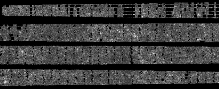
Figure 1.— Density of galaxies in stripe 11. The image of the stripe is split in 4 to preserve the aspect ratio. The width of the stripe is 2.5 degrees. The black pixels represent regions containing no objects. They are masked out due to bad field quality, seeing or bright stars. The narrowing of the stripe towards the left and right edge is due to the SDSS stripe geometry which ensures that objects are not counted twice. The pieces of the rectangle masked out towards the ends of the stripes are covered by adjacent stripes.

2.1. Building the Sample Database

From the current photometric data in the SDSS archives we extract eight stripes for our analysis. These stripes combine to form approximately five coherent regions on the sky which range from approximately 90 degrees to about 120 degrees in length. In the nomenclature of the SDSS these stripes are designated the numbers 10–12, 35–37 and 76 and 86. The last two stripes come from the southern component of the survey. All data from these stripes have been designated as having survey quality photometric observations and astrometry. In total these stripes add up close to 20 million galaxies and are accessible through the SDSS Science Archive (Thakar et al., 2001).

Currently, there are two versions of the SDSS science archive running at Fermilab and remotely accessible to the collaboration. The “chunk” database contains stripes that have passed through the target selection process for identifying candidates for spectroscopic followup but with only photometry that was available when the spectroscopic target selection was run on the region (i.e. photometry for which the calibrations were not necessarily optimal). The “staging” database has the latest photometric data (for this paper we use the ver. 5.2.8 of the photometric pipeline) but without the full target selection information. For our purposes the quality of the photometric measurements is important but the target selection is completely irrelevant and thus we take our sample from the staging database.

In order to be able to efficiently store, search and select galaxies from the catalog, we create a local database using Microsoft’s SQL Server. The relevant properties (position, redshift, galaxy type, absolute and apparent magnitudes) of all galaxies in the staging database were stored in this database server. The regions of the sky surveyed by these data, the seeing of the observations as a function of position on the sky and the position of bright stars that must be masked out when defining the survey geometry were all calculated internally from this data set.

From these data we restrict our sample to galaxies brighter than $r^{*}=21$. At this magnitude limit the star-galaxy separation is sufficiently accurate that it will not affect the angular clustering measures (Scranton et al., 2003) and the photometric redshift errors are typically less than $\sigma=0.06$ (Csabai et al., 2002). Applying this magnitude limit yields approximately 13 million galaxies from which to estimate the clustering signal. The sample was further restricted by excluding those regions of the stripes affected by the wings of bright stars or that were observed with poor seeing. Figure 1 shows the density of galaxies in stripe 11 with the masks over-plotted. Fields with seeing worse than $1.7^{\prime\prime}$ and a $3^{\prime}\!\!\times{}\!3^{\prime}$ neighborhood around all bright stars with $r^{*}<14$ were discarded.

We note that these selections were all accomplished by applying a series of SQL queries to the database rather than progressively pruning a catalog of galaxies. The boundaries of the stripes, the seeing on a field-by-field basis and all bright stars were stored in the local database, so that masks could be generated on the fly over the area to be analyzed. As such the selection criteria that were applied to the database could be optimized in a relatively short period of time.

2.2. Clustering from a Volume Limited Sample

Often the clustering evolution of galaxies, particularly that defined by angular clustering studies, is characterized as a function of limiting magnitude. While observationally this is simple to determine, the results of these analyzes are often difficult to interpret because in a magnitude limited sample the mix of the spectral types and absolute luminosities of galaxies is redshift dependent. We are, essentially, looking at the clustering properties of different types of galaxies as a function of limiting magnitude. The models to account for the clustering signal must, therefore, also be able to describe the evolution of the distribution of galaxies. Ideally we would separate out the effects of population mixing and study the evolution of angular clustering in terms of the intrinsic properties of galaxies (i.e. rest-frame color and luminosity), along with their distances. We can accomplish this if we use the photometric redshifts to select a volume limited sample of galaxies (i.e. one with a fixed absolute magnitude range as a function of redshift).

The SDSS Early Data Release photometric redshift catalog by Csabai et al. (2002) is based on techniques (Budavári et al., 2000, 1999; Csabai et al., 2000; Connolly et al., 1999) that estimate the physical parameters describing the galaxy samples in a self-consistent way. The relationship for the EDR data set is applied to the photometric data selected from the imaging stripes and the spectral types, absolute magnitudes and k-corrections are stored within a database together with the photometric and positional information. All derived quantities assume an $\Lambda$ cosmology with $h=0.7$, $\Omega_{\rm{}M}=0.3$ and $\Omega_{\Lambda}=0.7$.

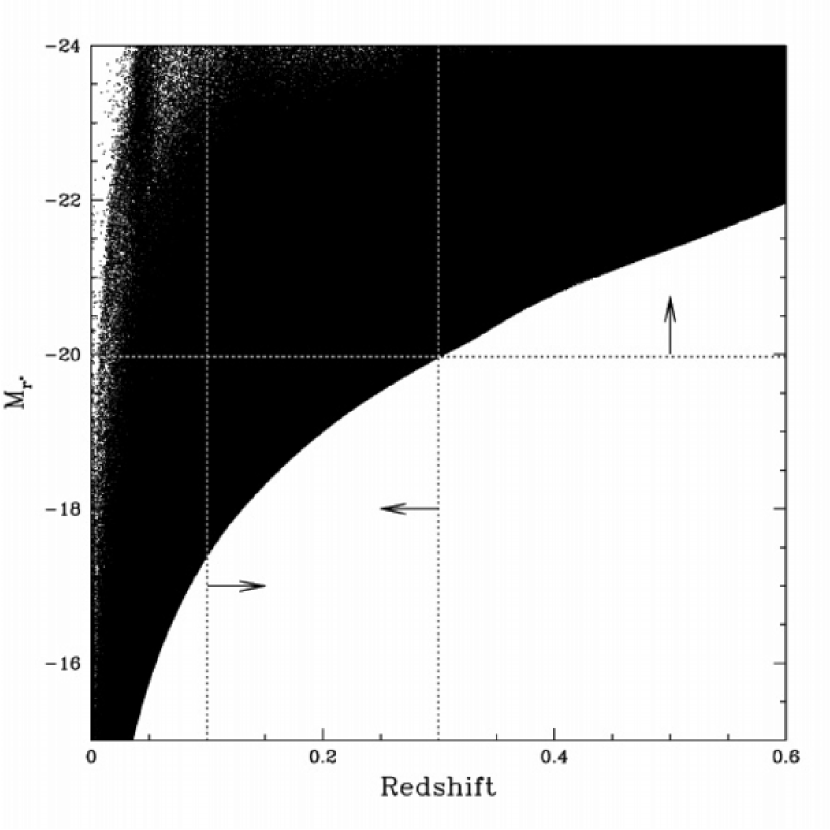
Figure 2.— Absolute $r^{*}$ magnitude vs. redshift relation as derived from the photometric redshift catalog. The dotted lines show our selection for the volume limited sample out to redshift 0.3.

Figure 2 illustrates how the absolute magnitude limits in the $r^{*}$ band vary as a function of redshift. These absolute magnitude boundaries are well defined, as a function of redshift, by the galaxies within our sample. In this paper we study a volume-limited sample that extends out to a redshift $z=0.3$ with limiting absolute magnitude $M_{r^{*}}=-19.97$. We further restrict the data set to those galaxies more distant than redshift $z=0.1$. The reason for this lower redshift limit is that the main spectroscopic galaxy sample will contain many of the low redshift galaxies, so using photometric redshift estimates is not necessary. Also the fractional error in $z$ becomes large at lower redshifts due to uncertainty in the phototometric redshifts. The final catalog size is over 2 million galaxies.

2.3. Rest-frame Selected Subsamples

To analyze how angular clustering changes with luminosity in Section 3, the volume limited sample is divided into 3 absolute magnitude bins. These subsamples represented by $M_{1}$, $M_{2}$ and $M_{3}$ have limiting absolute magnitudes $M_{r^{*}}\!>\!-21$, $-21\!>\!M_{r^{*}}\!>\!-22$ and $-22\!>\!M_{r^{*}}\!>\!-23$ respectively. The size of these subsets decrease by approximately a factor of two as a function of increasing luminosity.

For the type dependent selection we utilize the continuous spectral type parameter $t$ from the photometric redshift estimation. This essentially encodes the rest-frame colors of the galaxies as there is a direct one-to-one mapping between the type $t$ and the spectral energy distribution (SED) of the galaxy. The value $t=0$ represents a template galaxy that is as red as the elliptical spectrum of Coleman, Wu & Weedman (1980); as $t$ increases the galaxy type becomes progressively later. In Section 3, we subdivide by spectral class breaking the luminosity classes into four subgroups (each with comparable numbers of galaxies). The cuts in the spectral type parameter $t$ from red to blue are $t\!<\!0.02$, $0.02\!<\!t\!<\!0.3$, $0.3\!<\!t\!<\!0.65$ and $t\!>\!0.65$. The cuts are defined as the $T_{1}$, $T_{2}$, $T_{3}$ and $T_{4}$ subsamples respectively. Our selection is motivated by the spectral energy distributions of Coleman, Wu & Weedman (1980). The first class consists of galaxies with SEDs similar to the CWW elliptical template (Ell), the second, third and fourth classes contain a broader distribution of galaxy types approximately corresponding to Sbc, Scd and Irr types, respectively. The distribution of types and our classification are shown in Figure 3 and 4.

Figure 3.— The distribution of spectral type is bimodal. The small arrows hanging from the top axis illustrate our subsamples selected by spectral type. The cut between the 2 reddest and bluest classes at type $t=0.3$ (equivalent to rest-frame $u^{*}-r^{*}=2$) splits the distribution into 2 halves of similar sizes.

3. The Angular Correlation Function

The properties of the angular correlation function and the estimators used to measure it from photometric catalogs have been extensively discussed in the astronomical literature (Kerscher et al., 2000). The probability of finding galaxy within a solid angle $\delta\Omega$ on the celestial plane of the sky at distance $\theta$ from a randomly chosen object is given by (Peebles, 1980)

$$\delta{}P=n\ [1+w(\theta)]\ \delta\Omega,$$ (1)

where $n$ is the mean number of objects per unit solid angle. The angular two-point correlation function $w(\theta)$ basically gives the excess probability of finding an object compared to a uniform Poisson random point process.

Traditionally the observations are compared to random catalogs that match the geometry of the survey. The computation usually consists of counting pairs of objects drawn from the actual and random catalogs and applying a minimum variance estimator such as that defined by Landy & Szalay (1993) or Hamilton (1993). In this study, we use the Landy-Szalay estimator (Landy & Szalay, 1993) as

$$w_{LS}=\frac{\rm{}DD-2DR+RR}{\rm{}RR},$$ (2)

where DD, RR and DR represent a count of the data-data, random-random and data-random pairs with $\theta$ angular separation summed over the entire survey area.

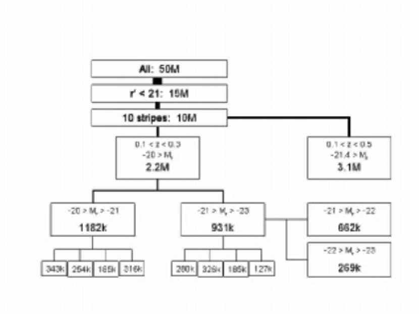
Figure 4.— Our classification and selection criteria are shown in this figure along with the number of galaxies in the subsamples.

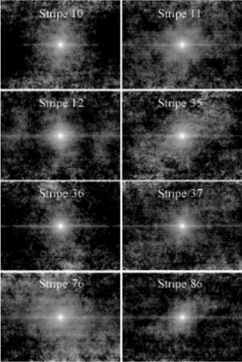
Figure 5.— The 2-dimensional correlation functions are shown for all 8 stripes on logarithmic scale. The correlation function is expected to be isotropic. Its sensitivity to artifacts in the data makes it an excellent diagnostic tool. The horizontal direction is the scan direction, along the stripe. The elongated streak at zero lag is related to the flat-field vector (see text). Note that the plots have parity symmetry through the origin, thus any half of the 2D space contains all the information for computing $w(\theta)$.

3.1. Estimating $w(\theta)$ with a Fast Fourier Transform

Even though distances on the sky are easy to compute mathematically, measuring the correlation function is not a trivial task, especially when it comes to large surveys. It’s easy to see that any naive algorithm implementing the estimator in Eq. (2) scales with the square of the number of objects $N$ in the survey, ${\cal{}O}(N^{2})$. It, therefore, becomes progressively more expensive in computational power to apply these techniques to data the size of the SDSS samples.

We propose a novel method to estimate $w(\theta)$ using the Fast Fourier Transform (e.g. in Press et al., 1992, hereafter FFT), which scales as ${\cal{}O}(N\log{}N)$, a significant improvement over the naive approach. The principle behind this is to group all galaxies into small cells within a grid and analyze this matrix instead of the point catalog. The implementation of this FFT approach called eSpICE is a Euclidean version of SpICE by Szapudi, Prunet & Colombi (2001). A discussion on its properties and scalings is given elsewhere (Szapudi et al., 2003). Here we present an application of eSpICE to the SDSS galaxy angular clustering and limit our discussion of the algorithm to only an outline of how the method works.

To apply a standard FFT analysis to the problem we operate in Euclidean space. In other words, Euclidean distances are computed instead of the correct angular separation. Given that we only examine separations of less than 2 degrees, the maximum relative distance error introduced by the use of the Euclidean approximation is only 0.00005. This has a negligible effect on the accuracy of our analysis, and the use of Euclidean distances increases the speed of the algorithms significantly. We use SDSS survey coordinates ($\mu,\nu$) to define the position of an object within a stripe. These coordinates are defined locally for each stripe. As the individual stripes comprise great circles on a sphere the survey coordinates along these great circles are close to Euclidean (i.e. in this coordinate system every stripe looks as if it were equatorial). In fact for equatorial stripes 10 and 82, the ($\mu,\nu$) coordinates are the same as (RA, Dec). Beyond the above data grid of galaxies, we need to describe the geometry of the survey area. This is done by a second grid, with the same dimensions that describes the survey boundaries. We call this the window grid because it is 1 if the pixel is entirely inside the boundaries and 0 otherwise. In this way we can also incorporate arbitrarily complex masks (e.g. for excluding regions around bright stars) as they are simply applied to the window grid. The data and window grids are then padded with zeros up to the maximum angular scale to avoid aliasing in the Fast Fourier Transform. Finally, eSpICE is used to calculate the two-point correlation function directly.

Our approach is to apply this algorithm to one stripe at a time. The data and window matrices are constructed by querying the SQL database to select the appropriate galaxies and masks. From these data we calculate the two-dimensional angular correlation function for all eight stripes. Figure 5 shows the 2D correlation function for all stripes used in this analysis. We find that the 2D correlation function is an extremely sensitive diagnostic tool for identifying systematics within the photometric data. The correlation function is expected to be isotropic. Artifacts within the data or survey geometry distort this symmetry. This is seen, to varying degrees, in each of the eight 2D correlations functions. We find that within the 2D correlation function there is an elongated streak, at zero lag, along the scan direction which has structure on scales in excess of a few degrees. This arises due to errors in the flat-field vector.

In a drift-scan survey the flat field is a one-dimensional vector (orthogonal to the direction of the scan). Errors within the flat field tend, therefore, to be correlated along the scan direction (i.e. along the columns of a stripe). This effect is seen within all of the individual stripe correlation functions. As it is, by definition, a zero lag effect we can exclude it from the analysis by censoring this region of the 2D correlation function before azimuthally averaging the signal to get a 1D correlation function. We note, however, that even if we do not censor the data to remove this effect the result of averaging the correlation function azimuthally (and the fact that this elongated streak only affects a small fraction of the 2D correlation function) the results discussed in the following sections are not affected.

In total, the computation of the one-dimensional angular correlation function $w(\theta)$ takes less than 3 minutes for a stripe, which is several orders of magnitude faster than traditional two-point estimators. Having computed the correlation function for all stripes, we co-add the results by properly weighting with the number of galaxy pairs. At the same time the covariance of the signal is also estimated from the scatter between the different stripes Figure 6 shows the covariance matrix for the volume limited sample ($z<0.3$). The image of the matrix is normalized so that the diagonal elements are always white and the (off-diagonal) gray scale values represent the correlation between the bins. Because of the logarithmic sampling of $w(\theta)$, the neighboring bins are farther apart and hence correlate progressively less as we go to larger scales and thus to larger bins.

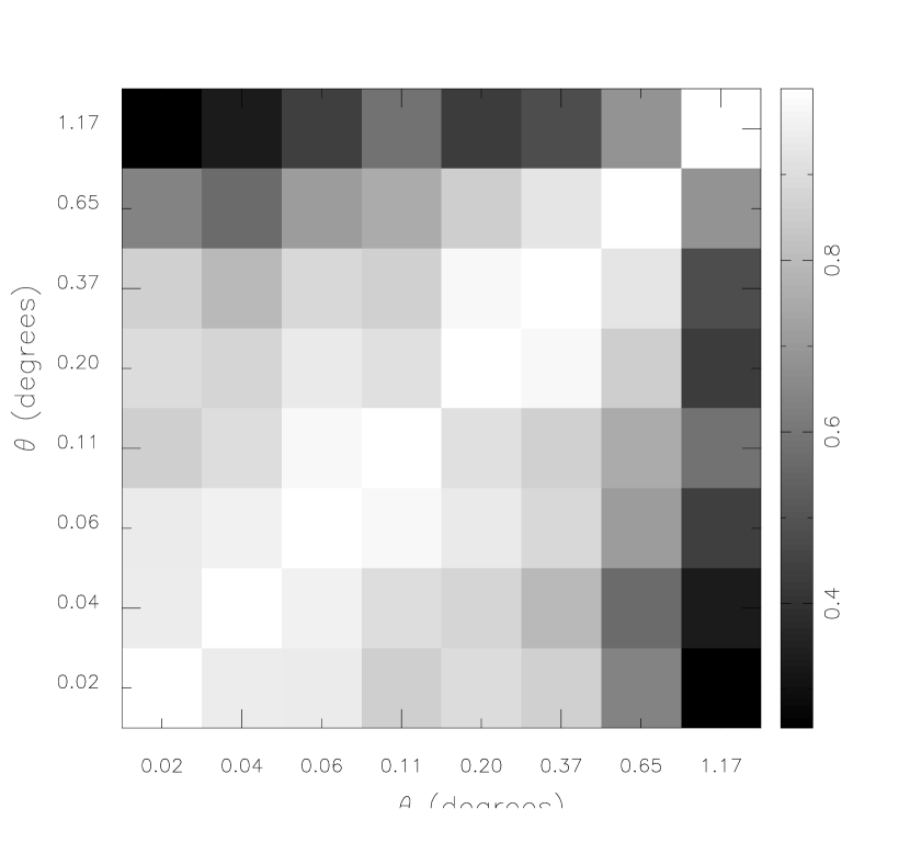
Figure 6.— The covariance matrix of the entire volume limited sample is normalized so that the diagonal elements are white and the grayscale values represent the correlations.

3.2. The Clustering Scale Length

With the measured correlation amplitudes as function of angular separation in hand, we can obtain a parametric form of the scaling. The amplitude and power of the correlation are calculated by fitting the usual formula,

$$w(\theta)=A_{w}\left(\frac{\theta}{\theta_{0}}\right)^{-\delta}.$$ (3)

Normalizing $\theta$ by $\theta_{0}=0.1^{\circ}$ enables the amplitude $A_{w}$ be directly compared with the figures showing $w(\theta)$ measurements; $A_{w}$ is essentially the value of the correlation function at $\theta_{0}$, since $A_{w}\equiv w(\theta_{0})$. The parameters $A_{w}$ and $\delta$ are estimated by minimizing the cost function

$$\chi^{2}(A_{w},\delta)=\frac{1}{N\!\!-\!\!2}\sum_{i,j=1}^{N}\Delta w_{i}\ C^{-1}_{ij}\Delta w_{j},$$ (4)

where $\Delta w_{i}=w_{i}-w(\theta_{i}|A_{w},\delta)$, $N$ is the number of bins and $C_{ij}$ is the covariance matrix. Although, $\chi^{2}(A_{w},\delta)$ is not quadratic in the parameter $\delta$, it is in $A_{w}$, thus the equation

$$\frac{\partial\chi^{2}}{\partial{}A_{w}}=0$$ (5)

can be solved analytically for $A_{w}$ to reduce the dimensionality of the problem. We then use a method by Brent (1973) (see Press et al., 1992) to search for the optimal value of $\delta$. The $\chi^{2}$ fit also provides information about the covariances of the estimated parameters that are shown as error ellipses in the next section.

Figure 7 illustrates the angular clustering in our fiducial sample of all galaxies within the volume limited sample. In the left panel, the correlation function $w(\theta)$ is shown along with the best power-law fit. The range in angular separation varies from 1 arcminute to 2 degrees. At a mean redshift for the volume-limited sample of $z=0.2$, $2^{\circ}$ corresponds to $\sim\!17\,h^{-1}\rm{}Mpc$. The error bars on the measurements are computed as one over the square root of the diagonal elements of the covariance matrix (e.g. shown in Figure 6). In the right panel of Figure 7, we plot the best fit parameters and their error ellipses. For the full volume-limited sample the best fit to the data has a slope of $\delta=0.84\pm{}0.02$ with an amplitude of $A_{w}=0.078\pm{}0.001$.

Figure 7.— Angular clustering in the fiducial sample of galaxies in the volume limited sample ($z<0.3$). The correlation function is shown (left panel) along with the best power-law fit using the formula $w(\theta)=A_{w}(\theta/0.1^{\circ})^{-\delta}$ (right panel).

Figure 8.— The clustering strength changes as a function of absolute magnitude without change in the slope. The correlation function and the parameter fits are shown in the left and right panels, respectively. The straight line represents the best fit to the fiducial sample in Fig. 7.

3.3. Clustering as a Function of Luminosity

The angular clustering of the galaxies in the three luminosity bins described in Section 3 are compared in Figure 8. As noted earlier, the left panel shows the correlation function, and the right panel gives the parameters of the power-law fits. The first section (I) of Table 1 presents the values and errors on these measured parameters. As expected, the more luminous galaxies are clustered more strongly: the amplitudes are roughly larger by a factor of 1.5 from one sample to the next and are measured to be $0.061\pm{}0.001$, $0.092\pm{}0.002$ and $0.138\pm{}0.004$. The slope of the correlation functions are consistent for all luminosity bins and with the fiducial value derived for the entire volume (the estimated slope parameters scatter around $\delta=0.84$).

3.4. Bimodality of $w(\theta)$ as a Function of Rest-frame Color

The type dependence of the correlation function is not as simple as that found for the luminosity classes. It is well known that different types of galaxies have different clustering behavior (Giovanelli et al., 1986). Red elliptical galaxies are more likely to be found in higher density regions than spirals. Here, we study the evolution of the angular correlation function with spectral type in two absolute magnitude ranges, $M_{r^{*}}\!>\!-21$ and $-21\!>\!M_{r^{*}}\!>\!-23$. Both of these yield approximately 1 million galaxies within our volume. Figure 9 shows how the clustering changes as a function of spectral type in the lower luminosity sample. The 2 reddest classes of the galaxy population ($T_{1}$ and $T_{2}$) are essentially indistinguishable, their clustering is significantly stronger than for the other classes or our fiducial results. The bluest 2 classes ($T_{3}$ and $T_{4}$) have approximately the same power-law exponents but with different amplitudes. Section II of Table 1 summarizes the results of parameter fitting, which is also seen in the right panel of Figure 9. The higher luminosity classes show the same basic trends but with a stronger correlation amplitude. The results of the type dependence of power law fits to the high luminosity class are given in Figure 10 and Table 1.

Figure 9.— The slope of the angular correlation function changes significantly as a function of SED type. The figures illustrate the trend in the lower luminosity bin with $M_{r^{*}}\!>\!-21$. Note the bimodality in slope: the reddest two classes have the same slope, and the bluest two classes have the same slope, but the red slope differs distinctly from the blue slope.

Figure 10.— The clustering results follow the same trend in the high luminosity bin with $-21\!>\!M_{r^{*}}\!>\!-23$ as in the lower luminosity bin seen in Figure 9 but the amplitudes are systematically larger.

4. The Correlation Length for Galaxies

4.1. Limber’s Equation

From the angular clustering we can derive the spatial correlation length, $r_{0}$, given the redshift distribution of the data (Peebles, 1980). This is accomplished by integrating over the comoving coordinate along two lines of sight $r_{1}$ and $r_{2}$, separated by the angle $\theta$, to calculate the projected angular correlations from the real-space correlation function $\xi(r)=(r/r_{0})^{-\gamma}$,

$$w(\theta)=\int\frac{r_{1}^{2}\Phi(r_{1})dr_{1}}{F(r_{1})}\int\frac{r_{2}^{2}\Phi(r_{2})dr_{2}}{F(r_{2})}\ \xi_{12},$$ (6)

where $\Phi(r)$ is the selection function and the factor $F(r)=1-kr^{2}$ accounts for the curvature of space. In the small angle approximation, the correlation function $\xi_{12}=\xi(r_{1}^{2}+r_{2}^{2}-2r_{1}r_{2}\cos\theta)$ becomes $\xi_{12}=\left(r/r_{0}\right)^{-\gamma}\left(\theta^{2}+u^{2}/r^{2}\right)^{-\gamma/2}$ using variables $2r=r_{1}+r_{2}$ and $u=r_{1}-r_{2}$. This simplifies the above integral, because one can separate out the part that has $u$ and arrive at

$$w(\theta)=r_{0}^{\gamma}H_{\gamma}\theta^{1-\gamma}\int\frac{r^{5-\gamma}\Phi^{2}(r)}{F^{2}(r)}dr,$$ (7)

where

$$H_{\gamma}={\frac{\Gamma(\frac{1}{2})\ \Gamma(\frac{\gamma-1}{2})}{\Gamma(\frac{\gamma}{2})}}.$$ (8)

We can rewrite the integral using redshift $z$ and its distribution. Substituting $r^{2}\frac{\Phi}{F}dr=\frac{dN}{dz}dz$ one gets the final integral of

$$w(\theta)=r_{0}^{\gamma}H_{\gamma}\theta^{1-\gamma}\int_{0}^{\infty}r^{1-\gamma}\left(\frac{dN}{dz}\right)^{2}\left(\frac{dr}{dz}\right)^{-1}dz$$ (9)

that may be compared to the measured quantities directly. We have assumed that the selection function and the redshift distribution are normalized to $\int{\frac{dN}{dz}}dz=1$, which can be easily achieved numerically.

4.2. Estimating $dN/dz$

To determine the correlation length, we need to estimate $dN/dz$. Given a photometric redshift and its random error, there is a conditional probability of having a galaxy at a certain true redshift. In addition, we need to incorporate the apparent magnitude limit and photometric redshift selection criteria in the estimate of the redshift distribution. The real redshift $z$ and the photometric redshift $s$ of a galaxy are different. We assume that $s=z+\nu$ where $\nu$ is the error and drawn from a normal distribution. Thus

$$P(s|z)=\frac{1}{\sqrt{2\pi\sigma^{2}}}\exp\left\{{-\frac{(s-z)^{2}}{2\sigma^{2}}}\right\},$$ (10)

where $\sigma$ determines the precision of the estimates. We need the inverse: what is the true redshift, given the photometric estimate. This may be obtained from Bayes’ theorem,

$$P(z|s)=\frac{P(z)\,P(s|z)}{P(s)},$$ (11)

where $P(z)$ is the true redshift distribution calculated from the LF that also depends on the apparent magnitude cuts.

Our volume limited sample is selected by a window function of photometric redshifts,

$$W(s)=\begin{cases}1&\text{if $s$ between 0.1 and 0.3,}\\ 0&\text{otherwise.}\\ \end{cases}$$ (12)

The conditional probability of having a galaxy in a sample selected by this window function is calculated by the integral over the distribution $P(s)$,

$$P(z|W) =\int\!\!ds\,P(s)\,W(s)\,P(z|s)$$ (13)

$$=P(z)\int\!\!ds\,W(s)\,P(s|z)$$ (14)

$$=P(z)\,W_{\sigma}(z),$$ (15)

where $W_{\sigma}(z)$ is the photometric redshift selection function convolved with the photometric redshift uncertainty.

Figure 11.— The redshift distribution is computed by adding the contributions of narrow $r^{*}$ intervals. The top panel (a) shows the number density of galaxies with $r^{*}$ between 18 and 18.2 as function of redshift, as derived from the luminosity function. The black shaded curve is the corresponding window function with $\sigma=0.05$. The product of these two, shown in panel (b), is the effective contribution of the magnitude bin. Panel (c) illustrates the final redshift histogram, which is the properly weighted sum of the products like the one above.

The precision of photometric redshifts is a strong function of the apparent magnitude. From the photometric redshift catalog, we compute the mean redshift errors $\sigma_{i}$ and the galaxy counts $n_{i}$ (for proper weighting) in $\Delta{}r^{*}=0.2$ wide magnitude bins. Using the LF by Blanton et al. (2003), we derive the redshift distributions $P_{i}(z)$ for the same magnitude bins up to $r^{*}=21$, which is the limiting magnitude in the sample. The final redshift distribution is the weighted average of these probabilities,

$$\bar{P}(z|W)\propto\sum_{i}n_{i}\,P_{i}(z)\,W_{\sigma_{i}}(z).$$ (16)

The top panel of Figure 11 illustrates the redshift distribution derived from the LF for galaxies with $18\!<\!\!r^{*}\!\!<\!\!18.2$ and a smoothed window $W_{\sigma}(z)$ with $\sigma=0.05$. The middle panel shows the effective contribution of this magnitude bin to the final $dN/dz$, which is plotted in the last panel.

4.3. Results for $r_{0}$

Applying the above probabilistic redshift distribution and substituting the power-law fits derived earlier, we find a correlation length for the full volume limited sample of $5.77\,h^{-1}\text{Mpc}$. Estimating the uncertainty of this value is not trivial. The statistical errors on the parametric fits to $w(\theta)$ are known and may be used to estimate the errors on the correlation length. These are estimated by calculating the scatter of the predicted $r_{0}$ measurements for 20,000 Monte-Carlo realizations of the fitting parameters, $A_{w}$ and $\delta$, based on their covariance matrix. For the full volume limited sample, we obtain $\Delta_{\text{rms}}=0.05\,h^{-1}\text{Mpc}$. However, the uncertainty on $r_{0}$ is also affected by the uncertainty in the redshift distribution. The primary source of change in the $dN/dz$ is the uncertainty in the LF parameters. We compute the partial derivatives $(\partial{}r_{0}/\partial{}\alpha)$, $(\partial{}r_{0}/\partial{}M_{*})$ and $(\partial{}r_{0}/\partial{}Q)$ numerically and propagate the quoted errors of Blanton et al. (2003). We find that the evolutionary parameter $Q$ makes the largest difference, the $r_{0}$ errors from the uncertainty of $M_{*}$ and $\alpha$ are negligible. For the fiducial $r_{0}$ value, we estimate an error of $\Delta_{\text{LF}}=0.09\,h^{-1}\text{Mpc}$. The dependence of $\sigma$ on the apparent magnitude was determined empirically using the actual measurements, thus the results are not affected by Malmquist bias.

Figure 12.— The correlation length $r_{0}$ is plotted as a function of luminosity (left) and spectral type (right panel). The error bars include both error terms added in quadrature.

In Figure 12, the correlation length is plotted as a function of luminosity (left panel) and SED type (right panel). The relation between $r_{0}$ and luminosity and spectral type are consistent with that observed directly from the angular data and from measures of the clustering length from spectroscopic surveys (Zehavi et al., 2002). Over an absolute magnitude range of $-19.97$ to $-22$, $r_{0}$ increases with luminosity from a value of $5.04\pm{}0.09$ to $7.87\pm{}0.24\,h^{-1}\text{Mpc}$, which is consistent with the increase observed by Zehavi et al. (2003).

The color dependence of $r_{0}$ (i.e. clustering as a function of spectral type) shows the expected increase in clustering length for early type galaxies. The values of the correlation length for the spectral type subsamples are given in Table 1. In the lower luminosity bin red, $T_{1}$, galaxies have a correlation length of $6.59\pm{}0.17\,h^{-1}\text{Mpc}$ for the $M_{r^{*}}>-21$ sample and the bluest galaxies, $T_{4}$, have a correlation length of $4.51\pm{}0.19\,h^{-1}\text{Mpc}$. The trend in this relation is again consistent with the observed dependence of the correlation length as a function of spectral and morphological type (Giovanelli et al., 1986).

5. Discussion

The interesting aspect of the luminosity and color dependent clustering is not that the observed clustering length scales with luminosity and color as this has been demonstrated from many different surveys. It arises from how the shape of the correlation function depends on luminosity and color. It is remarkable that the luminosity simply effects the amplitude of the correlation function and not the slope, whereas the type selection affects both the slope and amplitude. This is particularly intriguing when we note that we would expect an intrinsic correlation between the luminosity and spectral type of a galaxy.

Observationally, early type galaxies tend to reside in clusters of galaxies whereas later type galaxies are more often found in the field. We would expect, therefore, that early type galaxy samples would have more small separation pairs than samples selected for late type galaxies and that their resulting correlation functions would be steeper. This is consistent with the data except that we would expect there to be a smooth transition from early to late type galaxies and that the correlation function slope should smoothly change from a steep value of $0.96$ for the early types to the more shallow value of $0.68$ for the late types. What we observe, however, is that red galaxies (types $T_{1}$ and $T_{2}$) have a common slope of $\sim 0.1$ and blue galaxies (types $T_{3}$ and $T_{4}$) have a slope of $0.07$ (i.e. there does not appear to be a smooth transition).

We can, however, explain this behavior if we consider a simple model for the distribution of galaxy types. From Figure 3 we see that the type histogram for the galaxies is almost bimodal (Strateva et al., 2001; Hogg et al., 2003) with the distribution being well fit by two Gaussians. For simplicity we will denote these subclasses as “red” and “blue”. If the “red” and “blue” populations have distinct correlation functions (i.e. with different slopes), then any observed correlation function should simply come from mixing these populations. As we change the mix of “red” and “blue” galaxies then the resulting slope of the correlation function will also change. This is exactly what we observe with the correlation function as we move from the $T_{2}$ to $T_{3}$ selections.

If we selected galaxies only from either the “red” or “blue” sub-populations we would expect no change in the correlation function slope as all of the “red” or “blue” galaxies have a common correlation function. Again, this what we observe from the data. The slopes of the correlation functions for the $T_{1}$ and $T_{2}$ red samples are identical as are the correlation functions for the blue $T_{3}$ and $T_{4}$ samples. In reality, the color selection that we applied to the SDSS data (types $T_{1}$ through $T_{4}$) was not chosen to optimally separate two distinct populations of galaxies but rather to provide a simple subdivision of galaxies based on the CWW spectral energy distributions. We might expect there to remain some population mixing in our $T_{1}$, $T_{2}$, $T_{3}$ and $T_{4}$ color cuts. We observe this effect where the amplitude of the correlation function for the $T_{3}$ and $T_{4}$ classes are close but not identical; this would imply that the $T_{3}$ still contains a subset of the “red” galaxies.

The luminosity dependence can be explained if we note that the luminosity functions of the “red” and “blue” classes are identical for magnitudes brighter than $M_{r^{*}}=-20$ (Baldry et al., 2003). They deviate only for the faint end of the luminosity function (“blue” galaxies having a steeper faint end slope). Varying the luminosity cuts should not change the mix of the galaxy populations (unless we sample galaxies with $M_{r^{*}}>-20$). We would, therefore, expect the shape of the correlation function to be independent of the luminosity cuts (as is found from the data). Given this hypothesis if we selected a volume limited sample for galaxies with luminosities less that $M_{r^{*}}=-20$ we would expect to find a dependence on the slope with luminosity.

It is, therefore, remarkable that with such a simple model for the distribution of galaxies (i.e. just two classes with differing correlation functions) we can qualitatively describe the behavior of the correlation functions with color and luminosity. What is difficult to understand is why there would be a simple scaling of the amplitude of the correlation function with intrinsic luminosity as the spatial scales we sample are in the non-linear regime (i.e. a simple linear bias model is not necessarily appropriate). Identifying the physical mechanism that could give rise to the luminosity and type dependent bias that we observe remains an open question.

Table 1Power-law fits to correlation functions and correlation lengths

Sample	Luminosity	SED type	$N$	$A_{w}$	$\delta$	$r_{0}$
Fiducial	All	All	2,016	$0.078\pm{}0.001$	$0.84\pm{}0.02$	$5.77\pm{}0.05\pm{}0.09$
I	$M_{r^{*}}\!>\!-21$	All	1,098	$0.061\pm{}0.001$	$0.84\pm{}0.03$	$5.04\pm{}0.05\pm{}0.08$
	$-21\!>\!M_{r^{*}}\!>\!-22$	All	650	$0.092\pm{}0.002$	$0.85\pm{}0.04$	$6.26\pm{}0.08\pm{}0.10$
	$-22\!>\!M_{r^{*}}\!>\!-23$	All	268	$0.138\pm{}0.004$	$0.84\pm{}0.05$	$7.87\pm{}0.21\pm{}0.12$
II	$M_{r^{*}}\!>\!-21$	$t<0.02$	343	$0.112\pm{}0.004$	$0.96\pm{}0.05$	$6.59\pm{}0.14\pm{}0.10$
	$M_{r^{*}}\!>\!-21$	$0.02<t<0.3$	254	$0.109\pm{}0.005$	$1.02\pm{}0.06$	$6.28\pm{}0.24\pm{}0.09$
	$M_{r^{*}}\!>\!-21$	$0.3<t<0.65$	185	$0.072\pm{}0.008$	$0.66\pm{}0.12$	$5.90\pm{}0.51\pm{}0.10$
	$M_{r^{*}}\!>\!-21$	$t>0.65$	316	$0.047\pm{}0.003$	$0.68\pm{}0.09$	$4.51\pm{}0.18\pm{}0.07$
III	$-21\!>\!M_{r^{*}}\!>\!-23$	$t<0.02$	280	$0.161\pm{}0.007$	$0.96\pm{}0.05$	$7.91\pm{}0.36\pm{}0.12$
	$-21\!>\!M_{r^{*}}\!>\!-23$	$0.02<t<0.3$	326	$0.155\pm{}0.005$	$0.87\pm{}0.04$	$8.21\pm{}0.19\pm{}0.12$
	$-21\!>\!M_{r^{*}}\!>\!-23$	$0.3<t<0.65$	185	$0.093\pm{}0.010$	$0.70\pm{}0.15$	$6.75\pm{}0.56\pm{}0.11$
	$-21\!>\!M_{r^{*}}\!>\!-23$	$t>0.65$	127	$0.067\pm{}0.010$	$0.72\pm{}0.17$	$5.52\pm{}0.59\pm{}0.09$

References

- DR1; Abazajian et al. (2003) Abazajian, K., et al., 2003, in preparation
- Arnouts et al. (1999) Arnouts, S., Cristiani, S., Moscardini, L., Matarrese, S., Lucchin, F., Fontana, A., & Giallongo, E. 1999, MNRAS, 310, 540
- Baldry et al. (2003) Baldry, I.K., et al., 2003, in preparation
- Baugh et al. (1999) Baugh, C. M., Benson, A. J., Cole, S., Frenk, C. S., & Lacey, C. G. 1999, MNRAS, 305, L21
- Blanton et al. (2003) Blanton, M.R., et al., 2003, ApJ, in press
- Brent (1973) Brent, R.P., 1973, Algorithms for Minimization without Derivatives (Englewood Cliffs, NJ: Prentice-Hall), Chapter 5.
- Brunner, Szalay & Connolly (2000) Brunner, R.J., Szalay, A.S., Connolly, A.J., 2000, ApJ, 541, 527
- Budavári et al. (1999) Budavári, T., Szalay, A.S., Connolly, A.J., Csabai, I., & Dickinson, M.E., 1999, in Photometric Redshifts and High Redshift Galaxies, eds. R.J. Weymann, L.J. Storrie–Lombardi, M. Sawicki, & R. Brunner, (San Francisco: ASP), 19
- Budavári et al. (2000) Budavári, T., Szalay, A.S., Connolly, A.J., Csabai, I., & Dickinson, M.E., 2000, AJ, 120, 1588
- Coleman, Wu & Weedman (1980) Coleman, G.D., Wu., C.-C., & Weedman, D.W., 1980, ApJS, 43, 393
- Connolly et al. (1995a) Connolly, A.J., Csabai, I., Szalay, A.S., Koo, D.C., Kron, R.G., & Munn, J.A., 1995a, AJ, 110, 2655
- Connolly et al. (1998) Connolly, A.J., Szalay, A.S., Brunner, R.J., 1998, ApJ, 499, L125
- Connolly et al. (1999) Connolly, A.J., Budavári, T., Szalay, A.S., Csabai, I., & Brunner, R.J., 1999, in Photometric Redshifts and High Redshift Galaxies, eds. R.J. Weymann, L.J. Storrie–Lombardi, M. Sawicki, & R. Brunner, (San Francisco: ASP), 13
- Csabai et al. (2000) Csabai, I., Connolly, A.J., Szalay, A.S., & Budavári, T., 2000, AJ, 119, 69
- Csabai et al. (2002) Csabai, I., et al., 2002, accepted to AJ
- Firth et al. (2002) Firth, A. E. et al. 2002, MNRAS, 332, 617
- Fukugita et al. (1996) Fukugita, M., Ichikawa, T., Gunn, J.E., Doi, M., Shimasaku, K. & Schneider, D.P. 1996, AJ, 111, 1748
- Giovanelli et al. (1986) Giovanelli, R., Haynes, M.P., Chincarini, G.L., 1986, ApJ, 300, 77
- Gunn et al. (1998) Gunn, J.E., Carr, M.A., Rockosi, C.M., Sekiguchi, M., et al. 1998, AJ, 116, 3040
- Hamilton (1993) Hamilton, A.J.S., 1993, ApJ, 417, 19
- Hogg et al. (2001) Hogg, D.W., Finkbeiner, D.P., Schlegel, D.J., Gunn, J.E., 2001, AJ, 122, 2129
- Hogg et al. (2003) Hogg, D.W., et al., 2003, ApJ, in press
- Kerscher et al. (2000) Kerscher, M., Szapudi, I., Szalay, A.S., 2000, ApJ, 535, 13
- Landy & Szalay (1993) Landy, S.D., & Szalay, A.S., 1993, ApJ, 412, 64
- Lupton et al. (2003) Lupton, R.H., et al., 2003, in preparation
- Magliocchetti & Maddox (1999) Magliocchetti, M., & Maddox, S.J., 1999, MNRAS, 306, 988
- Norberg et al. (2001) Norberg, P., et al., 2001, MNRAS, 328, 64
- Peebles (1980) Peebles, P.J.E., 1980, in Large-Scale Structure of the Universe, 174
- Pier et al. (2002) Pier, J.R., et al., 2002, AJ, in press, astro-ph/0211375
- Press et al. (1992) Press, W.H., Teukolsky, S.A., Vetterling, W.T., & Flannery, B.P., 1992, in Numerical Recipes in C (Cambridge University Press)
- Roukema et al. (1999) Roukema, B. F., Valls-Gabaud, D., Mobasher, B., & Bajtlik, S. 1999, MNRAS, 305, 151
- Scranton et al. (2003) Scranton, R., et al., 2003, in preparation
- Smith et al. (2002) Smith, J.A., et al., 2002, AJ, 123, 2121
- Stoughton et al. (2002) Stoughton, C., et al., 2002, AJ, 123, 485
- Strateva et al. (2001) Strateva, I., et al., 2001, AJ, 122, 186
- Szapudi, Prunet & Colombi (2001) Szapudi, I., Prunet, S., & Colombi, S., 2001, ApJ, 561, 11
- Szapudi et al. (2003) Szapudi, I., et al., 2003, in preparation (eSpICE)
- Teplitz et al. (2001) Teplitz, H. I., Hill, R. S., Malumuth, E. M., Collins, N. R., Gardner, J. P., Palunas, P., & Woodgate, B. E. 2001, ApJ, 548, 127
- Thakar et al. (2001) Thakar, A.R., Kunszt, P.Z., Szalay, A.S., 2001, in Mining the Sky, eds. A.J. Banday et al., (Garching: ESO Astrophysics Symposia, Proceedings 2000. XV), 624
- Totsuji & Kihara (1969) Totsuji, H., & Kihara, T., 1969, PASJ, 21, 221
- SDSS; York et al. (2000) York, D.G., et al., 2000, AJ, 120, 1579
- Zehavi et al. (2002) Zehavi, I., et al., 2002, ApJ, 571, 172
- Zehavi et al. (2003) Zehavi, I., et al., 2003, in preparation