The core/envelope symmetry in pulsating stars

Abstract

We demonstrate that there is an inherent symmetry in the way high-overtone stellar pulsations sample the core and the envelope, which can potentially lead to an ambiguity in the asteroseismologically derived locations of internal structures. We provide an intuitive example of the source of this symmetry by analogy with a vibrating string. For the stellar case, we focus on the white dwarf stars, establishing the practical consequences for high-order white dwarf pulsations both analytically and numerically. In addition, we verify the effect empirically by cross-fitting two different structural models, and we discuss the consequences that this approximate symmetry may have for past and present asteroseismological fits of the pulsating DBV, GD 358. Finally, we show how the signatures of composition transition zones that are brought about by physically distinct processes may be used to help alleviate this potential ambiguity in our asteroseismological interpretation of the pulsation frequencies observed in white dwarf stars.

1 Astrophysical context

Asteroseismology is the study of the internal structure of stars through their pulsation frequencies. The distribution of the observed pulsation periods is theoretically determined entirely by the run of two fundamental frequencies in stellar models: the buoyancy, or Brunt-Väisälä frequency and the acoustic, or Lamb, frequency. For nonradial $g$-mode pulsations in white dwarfs – the only modes so far observed in these stars – the buoyancy frequency is the dominant physical quantity that determines the pulsation periods, reflecting the internal thermal and mechanical structure of the star. A considerable body of work by numerous investigators has focussed on the signature that core properties, such as the crystallized mass fraction and the C/O abundance distributions, and envelope properties, such as diffusion profiles and surface layer masses, have on the pulsation frequencies. Unambiguous interpretation of the distribution of periods is hindered by the difficulty of disentangling the signatures of structures in the deep core from those in the envelope.

It is well known both analytically and numerically that the separation between the periods of consecutive radial overtones approaches a constant value for high-overtone modes, so one might think that these periods do not actually contain information about the internal structure of the star. The resolution of this apparent paradox is that in general there are sharp features in the Brunt-Väisälä frequency for which the modes may not be considered to be in the asymptotic limit, and the presence of these features perturbs the periods so that the period spacings are no longer uniform, an effect which is commonly referred to as ‘mode trapping’. Thus, these deviations from uniform period spacing contain information about sharp features in the Brunt-Väisälä frequency, and can be used to discern internal structure in the star, such as the locations of composition transition zones. To date, almost all analyses of observed mode trapping in white dwarf pulsators have focussed on determining the thicknesses of the various chemically pure envelope layers.

In particular, initial estimates of the He layer mass of the DBV GD 358 yielded $10^{-5.7}{M}_{\star}$ (Bradley & Winget, 1994), while more recent analyses (Metcalfe et al., 2000; Metcalfe et al., 2001) indicated a globally optimal fit with $M_{\rm He}=10^{-2.7}{M}_{\star}$ and a changing C/O profile at $M_{r}\sim 0.5$–$0.9\,{M}_{\star}$. However, the Metcalfe et al. analyses still found a local minimum in parameter space near $M_{\rm He}\sim 10^{-6}{M}_{\star}$. Most recently, Fontaine & Brassard (2002) calculated a grid of carbon core models that included a double-layered envelope structure, a result similar to the earlier time-dependent diffusion calculations of Dehner & Kawaler (1995). They were able to fit the observed periods of GD 358 down to a level of precision comparable to the fit of Metcalfe et al. (2001), without including any structure in the core. Their model had composition gradients at two locations in the envelope, near $10^{-3}$ and $10^{-6}{M}_{\star}$, and a chemically uniform core.

In this paper, we show that there is an inherent symmetry in the way in which high-overtone pulsations sample the cores and envelopes of the models, with the result that it may be possible to reconcile the differences between the fits mentioned above. Specifically, by expanding on the work of Montgomery (2003), we show that a sharp feature in the Brunt-Väisälä frequency in the core of the models can produce qualitatively the same mode trapping patterns as a corresponding feature in the Brunt-Väisälä frequency in the envelope, leading to a potential ambiguity in the interpretation of the observed periods. In the following sections, we demonstrate how this core/envelope mapping works for both DBV and DAV models, and we use it to suggest a re-interpretation of the previous and current fits for GD 358. As a further example, we show the results of cross-fitting between two structurally dissimilar models. Finally, we show what considerations allow this ‘symmetry’ to be broken.

2 Simple analogy: the vibrating string

In order to better illustrate the problem of $g$-mode oscillations in a white dwarf, we first imagine doing asteroseismology of a far simpler object, the vibrating string. As it turns out, all of the major results can be carried over to the astrophysical case.

2.1 The uniform string

If we take a uniform string with a constant ‘sound speed’ $c$, and assume a sinusoidal time dependence, then we obtain the following eigenvalue equation:

$$\frac{\partial^{2}\psi}{\partial x^{2}}+\frac{\omega^{2}}{c^{2}}\psi=0,\hskip 20.00003pt\psi(0)=0=\psi(L),$$ (1)

where $\psi(x)$ is the spatial part of the eigenfunction, $\omega$ is the eigenfrequency, and $L$ is the length of the string. The solution is given by

$$\psi(x)=A\sin(k_{n}x),\hskip 10.00002ptk_{n}=\frac{n\pi}{L},\hskip 10.00002pt\omega_{n}=k_{n}c,\hskip 10.00002ptn=1,2,3,\ldots$$ (2)

Thus, the spectrum of eigenfrequencies $\{\omega_{n}\}$ is equally spaced. If we now make a small position-dependent perturbation to the sound speed $c$, call it $\delta c(x)$, then the shift in frequencies may be calculated from a variational principle, yielding

$$\frac{\delta\omega_{n}}{\omega_{n}}=\frac{2}{L}\int_{0}^{L}dx\left(\frac{\delta c(x)}{c}\right)\sin^{2}(k_{n}x).$$ (3)

Finally, we may ask what the perturbation to the eigenfrequencies is for a new $\delta\tilde{c}(x)$ which is the reflection of $\delta c(x)$ about the midpoint of the string, i.e., $\delta\tilde{c}(x)=\delta c(\tilde{x})$, where $\tilde{x}\equiv L-x$:

$$\frac{\delta\omega_{n}}{\omega_{n}} = \frac{2}{L}\int_{0}^{L}dx\left(\frac{\delta c(\tilde{x})}{c}\right)\sin^{2}(k_{n}x)$$ (4)

$$= \frac{2}{L}\int_{0}^{L}d\tilde{x}\left(\frac{\delta c(\tilde{x})}{c}\right)\sin^{2}(k_{n}L-k_{n}\tilde{x})$$

$$= \frac{2}{L}\int_{0}^{L}d\tilde{x}\left(\frac{\delta c(\tilde{x})}{c}\right)\sin^{2}(k_{n}\tilde{x}).$$

From comparison of Eqs. 3 and 4, we see that $\delta c(x)$ and $\delta c(\tilde{x})$ produce identical sets of perturbed frequencies. Thus, from an asteroseismological standpoint, the two perturbations are degenerate and cannot be distinguished from one another. This is hardly surprising since we know that reflection about the midpoint of the string is a symmetry of the problem, i.e., it doesn’t matter which end of the string we call $x=0$, and how we choose it had better have no effect on the observed frequencies. Thus, the above symmetry must be present even if the perturbation $\delta c(x)$ is not small.

Figure 1: The frequency perturbations due to a bump in the sound speed for the nonuniform string: (upper panel) two perturbations which are mirror images of one another in the sense given by Eq. 8 (solid and dashed curves, respectively), both of which produce the same set of frequency perturbations (lower panel), shown as a function of overtone number $n$. The vertical dotted line in the top panel shows the the geometric location of the ‘centre’ of the string with respect to this reflection.

2.2 The nonuniform string

For the case when $c=c(x)$ is a function of $x$, Eq. 1 is still separable, but the $x$-dependence is no longer sinusoidal. However, if we consider only modes with relatively high overtone number ($n\gg 1$), then we may use the JWKB approximation to obtain

$$\psi_{n}(x)=A\frac{1}{\sqrt{k_{n}(x)}}\sin[\phi_{n}(x)],\hskip 20.00003ptk_{n}(x)=\frac{\omega_{n}}{c(x)},$$ (5)

where

$$\omega_{n}=\frac{n\pi}{\int_{0}^{L}dx\,c^{-1}(x)},\hskip 10.00002pt\phi_{n}(x)\equiv n\pi\frac{\int_{0}^{x}dx^{\prime}\,c^{-1}(x^{\prime})}{\int_{0}^{L}dx^{\prime}\,c^{-1}(x^{\prime})},\hskip 10.00002ptn=1,2,3,\ldots$$ (6)

Just as before, a small perturbation to the sound speed, $\delta c$, may be related to a change in the eigenfrequencies by

$$\frac{\delta\omega_{n}}{\omega_{n}}=\frac{2}{\int_{0}^{L}dx\,c^{-1}(x)}\int_{0}^{L}dx\,c^{-1}(x)\left(\frac{\delta c(x)}{c(x)}\right)\sin^{2}[\phi_{n}(x)].$$ (7)

Since the string is not uniform, it no longer possesses reflection symmetry about its midpoint. However, in analogy with the uniform case, we consider a reflection coordinate $\tilde{x}$ defined by

$$\phi_{n}(\tilde{x}) \equiv \phi_{n}(L)-\phi_{n}(x)$$ (8)

$$= n\pi-\phi_{n}(x).$$

As before, if we consider a ‘reflected’ perturbation $\delta\tilde{c}(x)/\tilde{c}(x)=\delta c(\tilde{x})/c(\tilde{x})$, then from Eq. 8 we have $dx\,c^{-1}(x)=-d\tilde{x}\,c^{-1}(\tilde{x})$, so we find that

$$\frac{\delta\omega_{n}}{\omega_{n}} = \frac{2}{\int_{0}^{L}dx\,c^{-1}(x)}\int_{0}^{L}dx\,c^{-1}(x)\left(\frac{\delta c(\tilde{x})}{c(\tilde{x})}\right)\,\sin^{2}[\phi_{n}(x)]$$ (9)

$$= \frac{2}{\int_{0}^{L}dx\,c^{-1}(x)}\int_{0}^{L}d\tilde{x}\,c^{-1}(\tilde{x})\,\left(\frac{\delta c(\tilde{x})}{c(\tilde{x})}\right)\,\sin^{2}[n\pi-\phi_{n}(\tilde{x})]$$

$$= \frac{2}{\int_{0}^{L}dx\,c^{-1}(x)}\int_{0}^{L}d\tilde{x}\,c^{-1}(\tilde{x})\,\left(\frac{\delta c(\tilde{x})}{c(\tilde{x})}\right)\,\sin^{2}[\phi_{n}(\tilde{x})],$$

which is identical to Eq. 7 if $\tilde{x}$ is replaced by $x$. Thus, the reflected perturbation produces the same set of frequency perturbations as did the original perturbation, so there again exists an ambiguity in inferring the structure of the string from its eigenfrequencies; this is illustrated in Fig. 1.

Figure 2: Upper panel: The change in mode periods as a function of overtone number $k$ due to a perturbation to the Brunt-Väisälä frequency at $M_{r}=0.5622\,{M}_{\star}$ (filled circles) and at a depth of $10^{-5.331}\,{M}_{\star}$ (open circles). Lower panel: residuals of the fit as a function of the position of the envelope bump in which the position of the core bump is kept fixed.

Finally, we note that this symmetry bears a close resemblance to the phenomenon of frequency aliasing in time-series analysis. If we consider the frequency perturbation to be a continuous function of the overtone number, such as the solid line in the lower panel of Fig. 1, then the fact that the spectrum of eigenfrequencies is discrete means that this curve is sampled only at an evenly spaced set of points. Now if the curve in the lower panel of Fig. 1 represents the frequency changes due to a perturbation in $\delta c/c$ at $x/L=0.30$, then the curve corresponding to the symmetric perturbation at $x/L\approx 0.87$ would be a highly oscillatory curve passing through the same set of integer values of $n$. However, since the eigenmodes sample this oscillatory curve only at integer values of $n$, this high frequency signal is ‘aliased’ back to lower frequencies, i.e., the solid curve in the lower panel of Fig. 1. In this way, a perturbation $\delta c/c$ at the point $\tilde{x}$ can, through aliasing, appear as if it originates at the point $x$.

3 White dwarf core/envelope symmetry

3.1 Analytical approach

We would now like to apply the ideas of the previous section to the pulsating white dwarf stars. We believe this should be possible since the adiabatic equations of oscillation of a spherically symmetric stellar model (in the Cowling approximation) can be reduced to a second-order differential equation, i.e., the $g$-mode pulsations can be reduced to a form which mimics that of the vibrating string. In particular, the oscillation equation may be written as (Deubner & Gough, 1984; Gough, 1993)

$$\frac{d^{2}}{dr^{2}}\psi(r)+K^{2}\psi(r)=0,\hskip 10.00002ptK^{2}\equiv\frac{\omega^{2}-\omega_{c}^{2}}{c^{2}}-\frac{L^{2}}{r^{2}}\left(1-\frac{N^{2}}{\omega^{2}}\right),$$ (10)

where $N$ is the Brunt-Väisälä frequency, $L^{2}\equiv\ell(\ell+1)$, $c$ is the sound speed, and $\omega_{c}$ is the acoustic cutoff frequency, which is usually negligible except near the stellar surface. For high overtone $g$-modes, we have $K\sim LN/\omega r$, and applying the JWKB approximation we find (Gough, 1993)

$$\psi_{k}(r)=A\frac{1}{\sqrt{K_{k}(r)}}\sin\left[\phi_{k}(r)+\frac{\pi}{4}\right],\hskip 5.0pt\omega_{k}=\frac{L}{\left(k-\frac{1}{2}\right)\pi}\,\int_{r1}^{r2}dr\,\frac{N}{r}$$ (11)

and

$$\phi_{k}(r)\equiv\left(k-\frac{1}{2}\right)\pi\,\frac{\int_{r1}^{r}dr^{\prime}\,|N|/r^{\prime}}{\int_{r1}^{r2}dr^{\prime}\,|N|/r^{\prime}},\hskip 10.00002ptk=1,2,3,\ldots$$ (12)

where $r_{1}$ and $r_{2}$ are the inner and outer turning points of the mode, respectively, and where we have switched from $n$ to $k$ to denote the radial overtone number. The major difference between this case and that of the string is that for the string the turning points were the same for every mode (i.e., the fixed endpoints), whereas for $g$-modes, the inner and outer turning points of the modes are weak functions of the mode frequency, so they are different for every mode. Thus, the reflection symmetry may not be as exact as it was for the string problem.

Figure 3: The mapping between points in the core ($x$-axis) and those in the envelope ($y$-axis) which produce similar mode trapping for moderate to high overtone modes. The solid line is the result of direct numerical fitting and the dashed line is the analytical prediction of Eq. (15), in which the inner and outer turning points, $r_{1}$ and $r_{2}$, have been taken to be the center and the surface, respectively.

If we consider a perturbation to the Brunt-Väisälä frequency $\delta N/N$, and we assume that the inner and outer turning points are fixed, then the problem is very similar to that of the nonuniform string, with the perturbations to the eigenfrequencies given by

$$\frac{\delta\omega_{k}}{\omega_{k}}=\frac{2}{\int_{r1}^{r2}dr\,N/r}\int_{r1}^{r2}dr\,\left(\frac{\delta N}{N}\right)\frac{N}{r}\sin^{2}\left[\phi_{k}(r)+\frac{\pi}{4}\right].$$ (13)

Similarly, the approximate reflection mapping between the points $r$ and $\tilde{r}$ is given by

$$\phi_{k}(r) = \phi_{k}(r_{2})-\phi_{k}(\tilde{r})$$ (14)

$$= \left(k-\frac{1}{2}\right)\,\pi-\phi_{k}(\tilde{r}),$$

which may be explicitly written as

$$\int_{r1}^{r}dr\,\frac{|N|}{r}=\int_{\tilde{r}}^{r2}dr\,\frac{|N|}{r}.$$ (15)

Essentially, the above equation says that points which are the same number of ‘wavelengths’ (nodes in the radial eigenfunction) from the upper and lower turning points are reflections of one another.

We remark that if we take $r_{1}=0$ and $r_{2}=R_{\star}$ in Eq. 12, then $\phi_{k}(r)$ becomes a monotonic increasing function between the centre and the surface, and could itself be used as a radial coordinate. In particular, if we define

$$\Phi(r)\equiv\frac{\int_{0}^{r}dr\,\frac{|N|}{r}}{\int_{0}^{R_{\star}}dr\,\frac{|N|}{r}},$$ (16)

then $\Phi(0)=0$ and $\Phi(R_{\star})=1$; since $\Phi$ is directly linked to the Brunt-Väisälä frequency, we will call it the ‘normalised buoyancy radius’. The radial coordinate $\Phi$ has the advantage that it makes the problem look quite similar to that of the uniform string: the ‘reflection mapping’ between the points $r$ and $\tilde{r}$ is given by $\Phi(r)=1-\Phi(\tilde{r})$, with the reflection point (‘centre of the string’) having $\Phi=\frac{1}{2}$. In addition, it can be shown that in the JWKB approximation the kinetic energy density per unit $\Phi$ is constant. Since this approximation is valid everywhere except at sharp features such as composition transition zones, a change in the kinetic energy density (as well as the ‘weight function’) plotted as a function of $\Phi$ gives us a clear indication of the amount of mode trapping which a mode experiences. We show examples of this in section 5.

For completeness, we mention that the analysis of the preceding paragraphs may also be carried out for high-order $p$-modes. In this case, we have $K\sim\omega/c$, with $\Phi$ given by

$$\Phi(r)\equiv\frac{\int_{r_{1}}^{r}dr\,c^{-1}}{\int_{r_{1}}^{r_{2}}dr\,c^{-1}}.$$ (17)

Since $\Phi$ is a function of the sound speed, $c$, we refer to it as the ‘normalised acoustic radius’. The reflection mapping is unchanged from the previous result, namely $\Phi(r)=1-\Phi(\tilde{r})$. If a range of $\ell$ values are observed, as is the case for the Sun, then this symmetry can be broken due to the fact that the lower turning point, $r_{1}$, is a function of $\ell$.

3.2 Full numerical treatment

In order to investigate this core/envelope symmetry in detail, we use a fiducial DB white dwarf model with the parameters ${M}_{\star}=0.6\,{\rm M}_{\odot}$, $T_{\rm eff}=24,000\,{\rm K}$, $M_{\rm He}=10^{-6}\,{M}_{\star}$, and we consider pulsation modes having $\ell=1$ with periods between 400 and 900 s. We choose the diffusion exponents for the C/He transition zone so as to make this transition zone as smooth as possible. The reason for this is that we wish the background model to be smooth so that the only bumps in the Brunt-Väisälä frequency are the ones which we put in by hand.

In Fig. 2, we show the change in mode periods caused by placing a bump in the Brunt-Väisälä frequency at a point in the core as well as those produced by a bump in the envelope: the filled circles in the upper panel correspond to a core bump at $M_{r}/{M}_{\star}=0.5622$, while the open circles are for a bump in the envelope at $\log(1-M_{r}/{M}_{\star})=-5.331$. We see that the shapes of the perturbations are qualitatively the same, and that both sets of perturbations are well fit by the same asymptotic formula (solid curve). In the lower panel, we show how the residuals change as we vary the position of the (induced) envelope bump in order to try to reproduce the period changes due to the (intrinsic) core bump, i.e., we move the envelope bump through a range of radii in order to examine whether we have found a global best fit. Clearly, not only is there one unambiguous global minimum which is an order of magnitude smaller than the other local minima, the residuals are a smooth function of the bump position, so we are justified in using a nonlinear fitting algorithm in order to find the local (and global) minimum at $\log(1-M_{r}/{M}_{\star})=-5.331$.

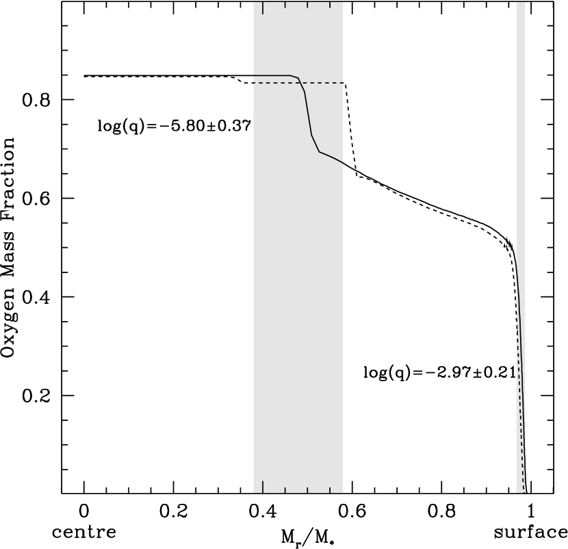
Figure 4: Theoretical internal oxygen profiles from Metcalfe et al. (2002) for a $0.65\,{\rm M}_{\odot}$ white dwarf model produced with standard semiconvective mixing (solid) and with complete mixing in the overshooting region (dashed) during central helium burning. The two shaded areas show the regions of the core where perturbations to the Brunt-Väisälä frequency can mimic perturbations in the envelope at values of $\log\,\,$q corresponding to those derived by Fontaine & Brassard (2002) for GD 358.

Using the above procedure, we can map out the corresponding pairs of core/envelope points in our equilibrium model, obtaining the solid curve in Fig. 3 (the dashed line is the result of using the analytical relation given by Eq. (15) with $r_{1}=0$ and $r_{2}=R_{\star}$). Thus, we see that a feature in the core at $M_{r}/{M}_{\star}\sim 0.5$ can mimic a feature in the envelope at $\log(1-M_{r}/{M}_{\star})\sim-5.5$. This is a very significant result because we a priori expect there to be both envelope bumps due to chemical diffusion as well as core bumps due to the prior nuclear burning history of the white dwarf progenitor.

For instance, in Fig. 4 we show evolutionary C/O profiles (Salaris et al., 1997) which result from assuming either standard semiconvective mixing (solid line) or complete mixing in the overshoot region (dashed line). Since the Brunt-Väisälä frequency depends on the radial derivative of these profiles, the regions of large slope at $M_{r}/{M}_{\star}\sim 0.5$ and $M_{r}/{M}_{\star}\sim 0.98$ will produce bumps in the Brunt-Väisälä frequency at these points. For the shaded regions in this figure, we have taken the quoted ranges of the He transition zones in the envelope of the model of Fontaine & Brassard (2002) and used the reflection mapping of Fig. 3 to indicate which regions in the core correspond to these envelope ranges. Almost eerily, these ranges correspond quite closely to those in which we would expect to see structure in the core. Thus, the possibility exists that Fontaine & Brassard are fitting ‘real’ structure in the core with assumed structure in the envelope. The reverse is also possible, of course, and at the very least the potential exists for the two signatures to become entangled with one another.

3.3 DA models

The above analysis can be directly applied to DAV models. For our fiducial model, we take ${M}_{\star}=0.60\,{\rm M}_{\odot}$, $T_{\rm eff}=12,000\,{\rm K}$, $M_{\rm He}=10^{-3}\,{M}_{\star}$, $M_{\rm H}=10^{-6}\,{M}_{\star}$. In order to make our background model as smooth as possible, we ignore the Ledoux term in the computation of the Brunt-Väisälä frequency; this reduces but does not eliminate the bumps due to the chemical transition zones. Finally, since these stars are cooler and therefore more degenerate, we consider longer period $\ell=1$ modes, of between 800 and 1300 s.

Figure 5: The same as Fig. 2, but for a DAV model. From the bottom panel, we see that the local minimum near $\sim-8.2$ (arrow 2) has residuals nearly as small as those at the minimum near $\sim-7.2$ (arrow 1), and that the residuals near $\sim-6.4$ are also fairly small. Thus, for all practical purposes, the core/envelope mapping is no longer single valued.

For the DAVs, we find a couple of surprises. First, as shown in Fig. 5, the mapping is no longer single-valued: there is more than one point in the envelope which is approximately mapped to a point in the core, and vice versa. In fact, there appear to be at least two and possibly more families of mappings which have approximately the same residuals. This is due to the fact that our background model already has two ‘bumps’ in it corresponding to the C/He and He/H transition zones, which our test bump is interacting with.

Figure 6: The same as Fig. 3, but for a DAV model. The dashed curve is the analytical result for the fiducial DAV model, and the two solid lines labelled 1 and 2 are the core/envelope mappings corresponding to minima 1 and 2 in Fig. 5. For reference, the dotted curve is the analytical result for our fiducial DBV model.

Second, as shown in Fig. 6, the core/envelope mapping is weighted much more toward the envelope than it is for the DBV models, i.e., a given point in the core is mapped to a point farther out in the envelope than it is in the DBV models. Physically, this is because the DAV model is cooler and has a more degenerate core, and therefore $N^{2}$ is smaller in its core. Thus, one has to move farther out from the centre in order to accumulate a given amount of phase in the sense of Eq. (15) or (16). The implications of this could be important, since a changing C/O profile in the range 0.5–0.9 ${M}_{\star}$ maps to an envelope point of $10^{-10}$–$10^{-8}$. Thus, such a C/O profile cannot mimic a hydrogen layer mass greater than $\sim 10^{-6}{M}_{\star}$, so the ambiguity in interpreting the origin of perturbations to the periods may be alleviated in the DAVs.

Finally, we wish to mention that at least one of the DAVs, BPM 37093, is theoretically predicted to have a partially crystallized core. In terms of seismology, the main effect of such a core would be to exclude the pulsations from the crystallized region (Montgomery & Winget, 1999a, b), effectively making the lower turning point, $r_{1}$, the upper boundary of the crystallized core. Thus, instead of running from 0 to 1, the horizontal axis in Fig. 6 would run from $M_{\rm Cr}/{M}_{\star}$, to 1, where $M_{\rm Cr}/{M}_{\star}$ is the crystallized mass fraction. This would tend to push the symmetry point for a given location in the core farther out into the envelope. Also, the higher mass of BPM means that its core will be more degenerate than that of the other DAVs, which will also push its symmetry mapping yet farther out into the envelope.

4 Cross-fitting two structural models

Empirical evidence that this symmetry in the white dwarf models may lead to some ambiguity in the interpretation of model-fits from various descriptions of the stellar interior was recently published in Fontaine & Brassard (2002) and Metcalfe (2003). To investigate the effects of this symmetry more directly, we performed several cross-fitting experiments with two different structural models – attempting to match the calculated pulsation periods from one model by using a structurally distinct model to do the fitting. In particular, we attempted to fit the carbon core double-layered envelope model periods from Table 1 of Fontaine & Brassard (2002) using the 5-parameter model of Metcalfe et al. (2001), which includes a single-layered envelope and an adjustable C/O core; we were able to find a match with root-mean-square period residuals of only $\sigma_{P}=1.26$ seconds (the optimal model parameters were identical to those found by Metcalfe (2003) for GD 358).

We may also use Fontaine & Brassard’s published results to turn the question around and see what goodness of fit they would obtain by attempting to fit the periods of our model. An upper limit on the root-mean-square residuals that may arise from such a comparison can be obtained by comparing the periods of the two optimal models for GD 358 from Metcalfe (2003) and Fontaine & Brassard (2002), leading to $\sigma_{P}\leq 1.26$ seconds. It is important to note that the double-layered envelope models may be able to match the periods from the adjustable C/O models even better than this with slightly different model parameters – a possibility that would even more clearly demonstrate a core/envelope symmetry.

Given the discussion of the previous sections, the results from the cross-fitting are not too surprising, since we are in essence fitting structure in the envelope of the Fontaine & Brassard model using structure in the core of our model located at the appropriate reflection point, and vice versa. The level of the residuals from our model-to-model comparison tells us directly what we have suspected for some time: the model-to-observation residuals for GD 358 ($\sigma_{P}\sim 1$ second) are dominated by structural uncertainties in the current generation of models, regardless of which type of model is used to do the fitting. This does not necessarily mean that the conclusions based on fitting from either of these models should be thrown out; it simply means that neither model is a complete description of the actual white dwarf stars, a statement that can hardly be considered controversial.

We can attempt to determine which of the two structural descriptions is closer to reality (or better describes the interior structure as sampled by the pulsations) by comparing the absolute level of the residuals for GD 358 from each model, corrected for the number of free parameters. The 4-parameter model of Fontaine & Brassard (2002) leads to $\sigma_{P}=1.30$ seconds when compared to the periods observed in GD 358. The Bayes Information Criterion (Koen & Laney, 2000) would lead us to expect the residuals of a 5-parameter fit to be reduced to 1.17 seconds just from the addition of an extra parameter. The 5-parameter model of Metcalfe (2003) does much better than this, with residuals of $\sigma_{P}=1.05$ seconds (an improvement equivalent to $4\sigma_{\rm obs}$) – suggesting that the internal C/O profile may be the more important of the two possible structures. Based on the results of our own experiments with double-layered envelope models (Metcalfe et al., in preparation) this possibility may be even more likely.

5 ‘Breaking’ the symmetry

In the previous sections, we have demonstrated that a core/envelope symmetry exists for high-overtone modes. Fortunately, this symmetry is approximate, and there are many ways in which it may be lifted or broken. For example, many of the DBVs appear to be higher overtone pulsators ($k\sim 10$), although this is not necessarily true for all of the observed modes in a given star, nor is it true of every member of the class. The DAVs as a class are not high-overtone pulsators, so this symmetry will be less of an issue for them. In addition, as shown in Fig. 6, the core/envelope mapping for DAV models is weighted more towards the envelope, so that the reflection point for many points in the core is in a region of the envelope where it may not overlap with the expected position of the chemical transition zones.

In addition, the core/envelope symmetry can be broken if we make additional assumptions. For instance, due to the different physical processes which produce them, the generic shape expected for the C/O profile in the core will be different from the expected shape of the C/He profile in the envelope. Using this information (parametrized in some form, for instance), we should be able to discern a core feature from an envelope feature. We show an example of this in Fig. 7, in which we see that the reflected bumps (lower panel) do indeed have different amplitudes and shapes from the actual bumps (middle panel) in the Brunt-Väisälä frequency [note that we have used the buoyancy radius, $\Phi$, as defined in Eq. 16, as our radial coordinate; along the top axis we use the more familiar $\log(1-M_{r}/{M}_{\star})$ ].

Figure 7: The bumps in the Brunt-Väisälä frequency (middle panel) which are produced by given chemical transition zones (upper panel), and the mirror image of these bumps under the reflection mapping (lower panel). We have taken the buoyancy radius $\Phi$ to be the radial variable; along the top axis of the upper panel we indicate the corresponding values of $\log(1-M_{r}/{M}_{\star})$.

The physical inputs used to generate Fig. 7 include a Salaris-like C/O profile (e.g., Salaris et al., 1997) and a two-tiered C/He Dehner-like envelope profile (Dehner & Kawaler, 1995). Furthermore, we have defined a ‘bump’, $\delta N/N$, as the fractional difference between the Brunt-Väisälä frequency calculated both with and without the Ledoux term (this term explicitly takes account of the effect which composition changes have on the value of $N^{2}$). While this yields reasonable results for the inner transition zones, for the outer C/He transition zone near $\log(1-M_{r}/{M}_{\star})\sim-6$ this prescription would greatly overestimate the importance of this bump. Instead, for this case we have taken $\delta N/N$ to be the fractional difference of the actual Brunt-Väisälä frequency and a third-order polynomial which smoothly joins onto the Brunt-Väisälä frequency on each side of the transition zone. With these definitions, we see that the inner C/O transition zone should produce the most dominant mode trapping feature, and that the inner C/He transition zone should produce the next most important feature, since these bumps are both the highest and the narrowest features present. In contrast, the outer C/He transition zone should have a relatively minor effect on the mode trapping.

We illustrate the mode trapping ability of this model in Fig. 8, in which we plot, again as a function of $\Phi$, the weight functions for $N^{2}$ (see Kawaler et al., 1985, their Eq. 8c) of the full numerical problem: the middle panel is the weight function for an $\ell=1$, $k=11$ mode, and the lower panel is that of an $\ell=1$, $k=21$ mode. In the upper panel we show the bumps corresponding to the composition transition zones, and in all panels we have shaded the regions containing the two largest bumps, since these should produce the strongest mode trapping. As we can see, this is certainly the case for the two modes we have selected: the modes show a marked change in amplitude in these shaded transition regions, but otherwise they propagate with essentially ‘constant amplitude’, i.e., their amplitudes evolve according to the JWKB formula.

So how does mode trapping help break the core/envelope symmetry? First, imagine that we wish to calculate the shift in periods due to all the bumps, not just to the two large ones we have highlighted. The $k=21$ mode is trapped between the two transition zones, so it will sample the bump at $\Phi\sim 0.37$ more strongly than modes such as the $k=11$ mode, which is not trapped in this region. Conversely, the $k=11$ mode has an enhanced amplitude in the outer layers ($\Phi\ga 0.6$), so it will sample the bump at $\Phi\sim 0.77$ more strongly than modes such as the $k=21$ mode, which is not trapped in this outer region. Thus, the effect which the smaller bumps have on the frequencies is strongly influenced by the mode trapping which the larger bumps produce. As a result, it should in principle be possible to discern whether there are in fact two bumps rather than one large one, what their relative locations are (e.g., both in the core, both in the envelope, or one each in the core and envelope), and what their relative strengths are.

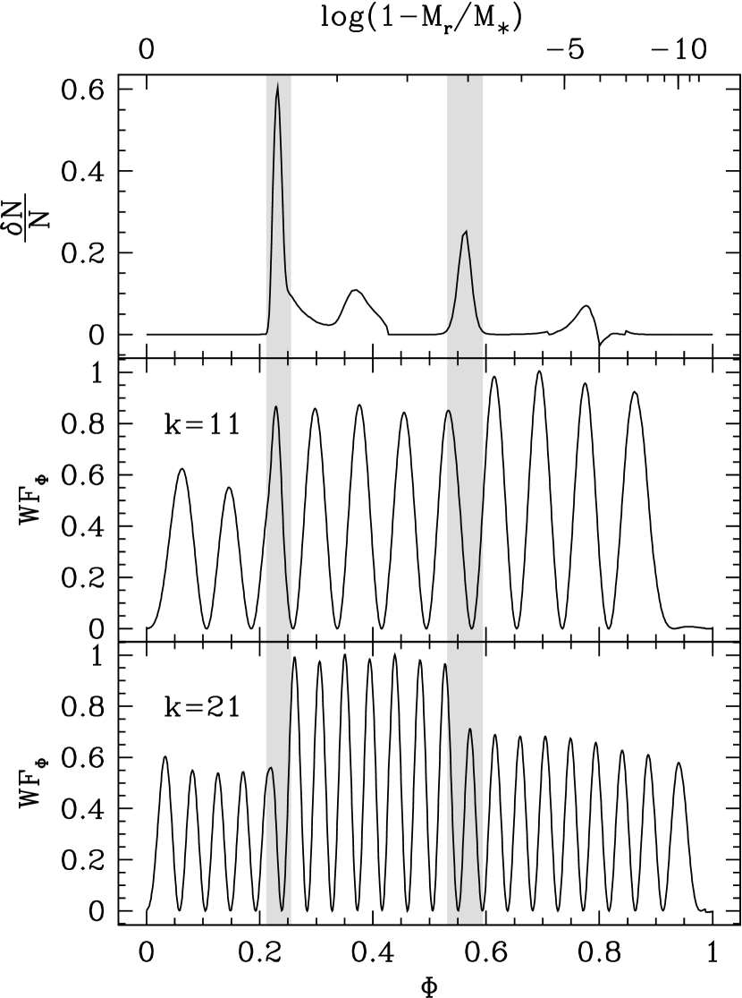
Figure 8: Examples of mode trapping of the eigenfunctions due to the composition transition zones. The upper panel shows the bumps in the Brunt-Väisälä frequency from Fig. 7 as a function of the buoyancy radius, $\Phi$, and the lower two panels show the weight function $WF_{\Phi}$ for two different modes, $k=11$ and $k=21$ (both with $\ell=1$). The shaded regions indicate the extent of the two most important transition zones; the differing amplitudes on each side of the transition zones clearly illustrates the mode trapping which these zones produce.

Additionally, the presence of modes of different $\ell$ may help in resolving this core/envelope symmetry, since the outer turning point is a function of $\ell$ for many of the modes. Also, constraints on the rotational splitting kernels (e.g., Kawaler et al., 1999) derived from rotationally split multiplets may be of help. In future calculations, we will attempt to address quantitatively the conditions under which it is possible to resolve the core/envelope symmetry, both in terms of the number of modes required as well as the physical assumptions needed regarding the shapes of the features to be resolved in the Brunt-Väisälä frequency.

6 Discussion & Conclusions

We have demonstrated, both analytically and numerically, that a symmetry exists which connects points in the envelope of our models with points in the core of our models. Specifically, we find that a sharp feature (‘bump’) in the Brunt-Väisälä frequency in the envelope of our models can produce the same period changes as a bump placed in the core, and we have numerically calculated this core/envelope mapping. While we have restricted ourself to the case of high-overtone white dwarfs which pulsate in $g$-modes, such a symmetry should be a generic feature of all high-overtone pulsators, whether they pulsate with $g$- or $p$-modes.

The specific motivation for much of our analysis has been the well-studied DBV, GD 358. Given its mass, stellar evolution theory leads us to expect that it has a C/O core, and that in some region of the core there should be a transition from a C/O mixture to a nearly pure C composition. If this transition begins at $\sim 0.5\,{M}_{\star}$, then it will produce a bump in the Brunt-Väisälä frequency at this point. As discussed in the previous sections, such a bump could be mimicked by an envelope transition zone with a depth of $\sim 10^{-6.0}\,{M}_{\star}$. Therefore, any incompleteness in the modelling of the core bump could be ‘corrected’ by a transition zone in the envelope placed at a depth of $10^{-6.0}\,{M}_{\star}$. This could explain the initial He layer determination of $10^{-6.0}\,{M}_{\star}$ by Bradley & Winget (1994) as well as the continuing presence of a local minimum near $\sim 10^{-6.0}\,{M}_{\star}$ in the current generation of models (Metcalfe et al., 2000; Metcalfe et al., 2001).

In addition, there is reason to believe that the actual C/He profile may be two-tiered, with a transition from pure C to a C/He mixture at $\sim 10^{-2}{M}_{\star}$ and another transition to pure He at $\sim 10^{-6}{M}_{\star}$ (Dehner & Kawaler, 1995; Córsico et al., 2002; Fontaine & Brassard, 2002); if this is the case, it is quite possible that the mode trapping effects of a C/O transition zone in the core could become entangled with those of the outer He transition zone. While additional considerations may break this core/envelope symmetry, we need to be aware of this aspect of the problem in order to make progress in modelling these stars.

In summary, we have shown that, for moderate to high overtone pulsators, there exists a symmetry in the mode trapping produced by features in the core and those in the envelope which can lead to ambiguity in determining the location of features such as composition transition zones. This may explain the present and previous fits for GD 358, and at the very least is something which must be taken into account in future asteroseismological fits.

References

- Bradley & Winget (1994) Bradley P. A., Winget D. E., 1994, ApJ, 430, 850
- Córsico et al. (2002) Córsico A. H., Althaus L. G., Benvenuto O. G., Serenelli A. M., 2002, A&A, 387, 531
- Dehner & Kawaler (1995) Dehner B. T., Kawaler S. D., 1995, ApJ, 445, L141
- Deubner & Gough (1984) Deubner F., Gough D., 1984, ARA&A, 22, 593
- Fontaine & Brassard (2002) Fontaine G., Brassard P., 2002, ApJ, 581, L33
- Gough (1993) Gough D. O., 1993, in Zahn J.-P., Zinn-Justin J., eds, Astrophysical fluid dynamics, Elsevier Science Publishers, Amsterdam, p. 399
- Kawaler et al. (1999) Kawaler S. D., Sekii T., Gough D., 1999, ApJ, 516, 349
- Kawaler et al. (1985) Kawaler S. D., Winget D. E., Hansen C. J., 1985, ApJ, 295, 547
- Koen & Laney (2000) Koen C., Laney D., 2000, MNRAS, 311, 636
- Metcalfe (2003) Metcalfe T. S., 2003, ApJ, 587, L43
- Metcalfe et al. (2000) Metcalfe T. S., Nather R. E., Winget D. E., 2000, ApJ, 545, 974
- Metcalfe et al. (2002) Metcalfe T. S., Salaris M., Winget D. E., 2002, ApJ, 573, 803
- Metcalfe et al. (2001) Metcalfe T. S., Winget D. E., Charbonneau P., 2001, ApJ, 557, 1021
- Montgomery (2003) Montgomery M. H., 2003, in Silvotti R., de Martino D., eds, Proceedings of the 13th European Workshop on White Dwarfs, Kluwer Academic Publishers, The Netherlands, p. 247
- Montgomery & Winget (1999a) Montgomery M. H., Winget D. E., 1999a, ApJ, 526, 976
- Montgomery & Winget (1999b) Montgomery M. H., Winget D. E., 1999b, in Solheim J.-E., Meištas E. G., eds, ASP Conference Series 169: Proceedings of the 11th European Workshop on White Dwarfs, ASP, San Francisco, p. 133
- Salaris et al. (1997) Salaris M., Dominguez I., García-Berro E., Hernanz M., Isern J., Mochkovitch R., 1997, ApJ, 486, 413