The DEEP2 Galaxy Redshift Survey: Clustering of Galaxies in Early Data

Abstract

We measure the two-point correlation function $\xi(r_{p},\pi)$ in a sample of 2219 galaxies between $z=0.7-1.35$ to a magnitude limit of $R_{\rm AB}=24.1$ from the first season of the DEEP2 Galaxy Redshift Survey. From $\xi(r_{p},\pi)$ we recover the real-space correlation function, $\xi(r)$, which we find can be approximated within the errors by a power-law, $\xi(r)=(r/r_{0})^{-\gamma}$, on scales $\sim 0.1-10$ $h^{-1}$ Mpc. In a sample with an effective redshift of $z_{\rm eff}=0.82$, for a $\Lambda$CDM cosmology we find $r_{0}$ $=3.53\pm 0.81$ $h^{-1}$ Mpc (comoving) and $\gamma=1.66\pm 0.12$, while in a higher-redshift sample with $z_{\rm eff}=1.14$ we find $r_{0}$ $=3.12\pm 0.72$ $h^{-1}$ Mpc and $\gamma=1.66\pm 0.12$. These errors are estimated from mock galaxy catalogs and are dominated by the cosmic variance present in the current data sample. We find that red, absorption-dominated, passively-evolving galaxies have a larger clustering scale length, $r_{0}$, than blue, emission-line, actively star-forming galaxies. Intrinsically brighter galaxies also cluster more strongly than fainter galaxies at $z\simeq 1$. Our results imply that the DEEP2 galaxies have an effective bias $b=0.96\pm 0.13$ if $\sigma_{8\ {\rm DM}}=1$ today or $b=1.19\pm 0.16$ if $\sigma_{8\ {\rm DM}}=0.8$ today. This bias is lower than what is predicted by semi-analytic simulations at $z\simeq 1$, which may be the result of our $R$-band target selection. We discuss possible evolutionary effects within our survey volume, and we compare our results with galaxy clustering studies at other redshifts, noting that our star-forming sample at $z\simeq 1$ has very similar selection criteria as the Lyman-break galaxies at $z\simeq 3$ and that our red, absorption-line sample displays a clustering strength comparable to the expected clustering of the Lyman-break galaxy descendants at $z\simeq 1$. Our results demonstrate that galaxy clustering properties as a function of color, spectral type and luminosity seen in the local Universe were largely in place by $z\simeq 1$.

1. Introduction

Understanding the nature of large-scale structure in the Universe is a key component of the field of cosmology and is vital to studies of galaxy formation and evolution. The clustering of galaxies reflects the distribution of primordial mass fluctuations present in the early Universe and their evolution with time and also probes the complex physics which governs the creation of galaxies in their host dark matter potential wells.

Since the first redshift surveys, the two-point correlation function, $\xi(r)$, has been used as a measure of the strength of galaxy clustering (Davis & Peebles 1983). $\xi(r)$ is relatively straightforward to calculate from pair counts of galaxies, and it has a simple physical interpretation as the excess probability of finding a galaxy at a separation $r$ from another randomly-chosen galaxy above that for an unclustered distribution (Peebles 1980). Locally, $\xi(r)$ follows a power-law, $\xi(r)$$=(r/r_{0})^{-\gamma}$, on scales $\sim 1-10$ $h^{-1}$ Mpc with $\gamma\sim 1.8$ (Davis & Peebles 1983; de Lapparent, Geller, & Huchra 1988; Tucker et al. 1997; Zehavi et al. 2002; Hawkins et al. 2003). The scale-length of clustering, $r_{0}$, is the separation at which the probability of finding another galaxy is twice the random probability. Locally $r_{0}$ is measured to be $\sim 5.0$ $h^{-1}$ Mpc  for optically-selected galaxies but depends strongly on galaxy morphology, color, type and luminosity (Davis & Geller 1976; Dressler 1980; Loveday et al. 1995; Hermit et al. 1996; Willmer, da Costa, & Pellegrini 1998; Norberg et al. 2001; Zehavi et al. 2002; Madgwick et al. 2003a).

The spatial clustering of galaxies need not trace the underlying distribution of dark matter. This was first discussed by Kaiser (1984) in an attempt to reconcile the different clustering scale lengths of field galaxies and rich clusters, which cannot both be unbiased tracers of mass. The galaxy bias, $b$, is a measure of the clustering in the galaxy population relative to the clustering in the underlying dark matter distribution. It can be defined as the square root of the ratio of the two-point correlation function of the galaxies relative to the dark matter: $b=(\xi/\xi_{\rm DM})^{1/2}$, either as a function of $r$ or defined at a specific scale (see Section 5.1). Observations of galaxy clustering have shown that the galaxy bias can be a function of morphology, type, color, luminosity, scale and redshift.

Using galaxy morphologies, Loveday et al. (1995) find that early-type galaxies in the Stromlo-APM redshift survey are much more strongly clustered than late-type galaxies. Their early-type sample has a larger correlation length, $r_{0}$, and a steeper slope than late-type galaxies. However, Willmer, da Costa, & Pellegrini (1998) show using data from the Southern Sky Redshift Survey (SSRS2, da Costa et al. 1998) that in the absence of rich clusters early-type galaxies have a relative bias of only $\sim 1.2$ compared with late-type galaxies. In their sample, red galaxies with $(B-R)_{0}>1.3$ are significantly more clustered than blue galaxies, with a relative bias of $\sim 1.4$. Zehavi et al. (2002) also studied galaxy clustering as a function of color, using data from the Sloan Digital Sky Survey (SDSS, York et al. 2000 ) Early Data Release, and find that red galaxies ($u^{*}-r^{*}>1.8$) have a larger correlation length, $r_{0}$, a steeper correlation function, and a larger pairwise velocity dispersion than blue galaxies. They also find a strong dependence of clustering strength on luminosity for magnitudes ranging from $M^{*}+1.5$ to $M^{*}-1.5$. Galaxy clustering for different spectral types in the 2dF Galaxy Redshift Survey (2dFGRS, Colless et al. 2001 ) is reported by Madgwick et al. (2003a); absorption-line galaxies are shown to have a relative bias $\sim 2$ times that of emission-line galaxies on scales $r=1$ $h^{-1}$ Mpc, declining to unity on larger scales. Absorption-line galaxies have a steeper correlation slope and a larger pairwise velocity dispersion. All of these results indicate that red, absorption-line, early-type galaxies are found predominantly in the more massive virialized groups and clusters in which the random velocities are large. Norberg et al. (2001) report that the correlation length of optically-selected galaxies in the 2dFGRS depends weakly on luminosity for galaxies fainter than $L^{*}$, the typical luminosity of a galaxy, but rises steeply with luminosity for brighter galaxies, with the most luminous galaxies being three times more clustered than $L^{*}$ galaxies. These results from local $z\sim 0$ surveys indicate that the strength of galaxy clustering is quite sensitive to different galaxy properties.

A critical test of both cosmological and galaxy evolution models is the redshift-dependence of galaxy clustering. The evolution of the dark matter two-point correlation function, $\xi_{\rm DM}(r,t)$, can be calculated readily and is strongly dependent on cosmology. In high-density models the clustering strength grows rapidly, while $\Lambda$CDM models show a more gradual evolution (e.g., Jenkins et al. 1998, Ma 1999) . However, the evolution of the galaxy two-point correlation function, $\xi(r,t)$, depends on the evolution of both the underlying dark matter distribution and the galaxy bias, which is expected to increase with redshift. Applying semi-analytic modelling of galaxy formation and evolution to dark matter simulations, Kauffmann et al. (1999b) present $\Lambda$CDM models with $r_{0}$ $\sim 4$ $h^{-1}$ Mpc  for the galaxy distribution at $z=1$ compared to $r_{0}$ $\sim 5.2$ $h^{-1}$ Mpc  locally. They predict a galaxy bias of $b\sim 1.2$ at $z=1$ for galaxies with $M_{B}<-19+5$ log $(h)$ but also find that the galaxy bias can be a strong function of luminosity, star-formation rate, galaxy type, and sample selection. Benson et al. (2001), who also apply semi-analytic modelling to $\Lambda$CDM dark matter simulations, predict a bias of $b=1.5$ at $z=1$ for galaxies with $M_{B}<-19.5+5$ log $(h)$. They also predict a similar morphology-density relation at $z=1$ to that seen locally.

Previous redshift surveys which have attempted to probe intermediate redshifts from $z=0-1$ have been hampered by small volumes and the resulting severe cosmic variance. Results from the Canada-France Redshift Survey (CFRS, LeFevre et al. 1996) are based on $\sim 600$ galaxies covering 0.14 degrees², the Norris Redshift Survey (Small et al. 1999) sparsely samples 20 degrees² with a survey of $\sim 800$ galaxies, Hogg, Cohen, & Blandford (2000) report on a sample of $\sim 1200$ galaxies in two very small fields, including the Hubble Deep Field, and Carlberg et al. (1997) present a survey of $\sim 250$ galaxies in a total area of 27 arcmin², finding that correlations found in their $K$-band data are generally greater than those found by optically-selected surveys. Small et al. (1999) compare results from several surveys which have measured the correlation length $r_{0}$ in the range $z=0-1$ and illustrate well the uncertainties in and discrepancies between these results. For an open CDM cosmology, the estimates of the comoving correlation length vary from $\sim 2-5$ $h^{-1}$ Mpc  at $z\simeq 0.4-0.6$. In particular, the CFRS survey found a much smaller correlation length at $z>0.4$ than the other surveys, which generally are consistent with weak evolution between $z=1$ and $z=0$. A significantly larger survey was undertaken by CNOC2 (Shepherd et al. 2001), who obtained redshifts for $\sim 5000$ galaxies over 1.44 degrees². Most relevant for our purposes may be Adelberger (1999), who present clustering results for a deep $R\leq 25.5,z\simeq 1$ sample of $\sim 800$ galaxies covering a total of 42.5 arcmin² in 5 fields; they quote a correlation length of $r_{0}$ $\sim 3$ $h^{-1}$ Mpc  for a $\Lambda$CDM cosmology, implying that their galaxy sample is an unbiased tracer of the mass at $z\simeq 1$. However, many of these surveys cover very small fields and are likely to underestimate the true clustering. There is a well-known systematic bias towards underestimation of $r_{0}$ in volumes which are small enough that all galaxies are part of a single large-scale structure and in which the large-scale modes cannot be sampled. Furthermore, cosmic variance will dominate any measure of clustering in volumes which are too small to be representative samples of the Universe (Davis et al. 1985).

Here we present early results on galaxy clustering in the DEEP2 Galaxy Redshift Survey (Davis et al. 2002), an $R-$band selected survey which was designed to study the universe at $z\simeq 1$ with a volume and sampling density comparable to local surveys. Our intent in this paper is to provide an initial measure of the galaxy clustering in our survey at using the first season of data and to investigate the dependence of the clustering on galaxy properties, splitting the sample by color, spectral type, and luminosity. To constrain galaxy evolution models, we measure the galaxy bias for the sample as a whole and the relative bias between subsamples. This is the first of several planned papers on galaxy clustering within the DEEP2 survey, and here we focus strictly on analysis of spatial correlations. Discussion of redshift-space distortions will appear in a subsequent paper (Coil et al. 2004). In the data from the first season of observations we measured 5042 redshifts with $z\geq 0.6$ in three fields with a total area of 0.72 degrees². The most complete field currently covers 0.32 degrees² and includes 2219 galaxies in the redshift range $z=0.7-1.35$, which we use as the primary data sample in this paper.

The outline of the paper is as follows: in Section 2 we briefly describe the survey, provide details of the observations, data reduction, and the data sample used here. Section 3 outlines the methods used in this paper, while Section 4 presents our results, both for the survey sample as a whole and for subsamples based on galaxy redshift, color, spectral type, and luminosity. In Section 5 we discuss galaxy bias and the relative biases between our subsamples, and we conclude in Section 6.

2. Data

2.1. The DEEP2 Galaxy Redshift Survey

The DEEP2 Galaxy Redshift Survey is a three-year project using the DEIMOS spectrograph (Faber et al. 2002) on the 10-m Keck II telescope to survey optical galaxies at $z\simeq 1$ in a comoving volume of approximately 6$\times$10⁶ $h^{-3}$ Mpc³. The completed survey will cover 3.5 degrees² of the sky over four widely separated fields to limit the impact of cosmic variance. The “1-hour-survey” (1HS) portion of the DEEP2 project will use $\sim 1$ hr exposure times to measure redshifts for $\sim 60,000$ galaxies in the redshift range $z\sim 0.7-1.5$ to a limiting magnitude of $R_{\rm AB}=24.1$ (all magnitudes in this paper are in the AB system; Oke & Gunn 1983 ). Photometric data were taken in $B,R$ and $I$-bands with the CFH12k camera on the 3.6-m Canada-France-Hawaii telescope. Galaxies selected for spectroscopy must additionally meet a color selection given approximately by $B-R\lesssim 2.35(R-I)-0.45$, $R-I\gtrsim 1.15$, or $B-R\lesssim 0.5$. This simple color-cut was designed to select galaxies at $z>0.7$ (details are given in Newman et al. 2004) and has proven effective in doing so. As discussed in Davis et al. (2002) this color-cut results in a sample with $\sim$90% of the objects at $z>0.7$, missing only $\sim$5% of the $z>0.7$ galaxies.

Each of the four DEEP2 1HS fields corresponds to a volume of comoving dimensions $\sim 20\times 80\times 1000$ $h^{-1}$ Mpc  in a $\Lambda$CDM model at a redshift of $z=1$. To convert measured redshifts to comoving distances along the line of sight we assume a flat cosmology with $\Omega_{\rm m}=0.3$ and $\Omega_{\Lambda}=0.7$. Changing cosmological models within the range allowed by recent WMAP analysis (Spergel et al. 2003) has only a modest influence on our results. We use $h={\rm{\it H}_{0}/(100\ km\ s^{-1}})$, and we quote correlation lengths, $r_{0}$, in comoving dimensions of $h^{-1}$ Mpc.

2.2. Observations and Data Reduction

This paper uses data from the first observing season of the 1HS portion of the DEEP2 survey, from August–October 2002. Three of the four DEEP2 fields were observed with a total of 68 custom-made slitmasks. Each mask has on the order of $\sim 120$ slitlets, with a median separation in the spatial direction between targeted galaxies of $\sim 6$″, and a minimum of 3″. Due to the high source density of objects, we are able to obtain spectra for $\sim 67\%$ of our targets. Three 20-minute exposures were taken on the DEIMOS spectrograph with a 1200 line mm^-1 grating for each slitmask, covering a spectral range of $\sim 6400-9100$ Å at an effective resolution $R\sim 5000$. The multiple exposures allow us to robustly reject cosmic rays from the data. Many of the slitlets in each mask are tilted to align with the major axis of the target galaxy to enable internal kinematic studies, and as a result we do not dither the telescope between exposures.

The data were reduced using a sophisticated IDL pipeline developed at UC-Berkeley, adapted from spectroscopic reduction programs developed for the SDSS (Burles & Schlegel 2004). To find the redshift of each galaxy, a $\chi^{2}$-minimization is used, where the code finds minima in $\chi^{2}$ between the observed spectrum and two templates; one is an artificial emission-line spectrum convolved with a broadening function to mimic a 1$\arcsec$ slit and 60 km s^-1 internal dispersion. The other template is a high signal-to-noise ratio absorption-dominated spectrum which is the average of many thousands of SDSS galaxies covering a rest wavelength range of 2700-9000 Å (Eisenstein et al. 2003; Burles & Schlegel 2004). The five most-likely redshifts are saved and used in a final stage where the galaxy redshift is confirmed by human interaction. Our overall redshift success rate is $\gtrsim$70% and displays only minor variation with color and magnitude ($<20$%), with the exception of the bluest galaxies ($R-I<0.4,B-R<0.5$) for which our redshift success rate is $\sim 35$%. These galaxies represent $\sim 25$% of our targeted sample and account for $\sim 55$% of our redshift failures.

The $\lambda$3727 Å [OII] doublet redshifts out of our spectral range at $z\sim 1.44$, and it is believed that all of our bluest ($R-I<0.4,B-R<0.5$) targeted galaxies for which we do not measure a redshift lie beyond this range. These galaxies have similar colors and source densities as the population at $z\simeq 2$ currently studied by C. Steidel and collaborators (private communication). If these galaxies were in our observable redshift window, it is almost certain that we would have measured a redshift, given that these blue galaxies must have recent star-formation and therefore strong emission lines.

Although the instrumental resolution and photon statistics of our data would suggest that we could achieve a redshift precision of $\sim 10$ km s^-1 in the rest frame of each galaxy, we find using galaxies observed twice on overlapping slitmasks that differences in the position or alignment of a galaxy within a slit and internal kinematics within a galaxy lead to an effective velocity uncertainty of $\sim 30$ km s^-1.

2.3. Data Sample

Here we present results from only the most complete field, centered at 02 hr 30 min +00 deg, for which we have observed 32 slitmasks covering $\sim 0.7$ degrees by $\sim 0.5$ degrees on the sky. We use data only from masks which have a redshift success rate of 60% and higher in order to avoid systematic effects which may bias our results. Figures 1 and 2 show the spatial distribution of galaxies on the plane of the sky and the window function for this field. The observed slitmasks overlap each other in two horizontal rows on the sky. Six of the masks have not as yet been observed in this pointing, leading to regions with lower completeness.

While we measure redshifts as high as $z=1.48$, for this paper we include only galaxies with $0.7<z<1.35$, a range in which our selection function is currently well defined. Our sample in this field and range contains 2219 galaxies, with a median redshift of $z=0.90$. At this median redshift the typical rest-frame wavelength coverage is $\sim 3400-4800$ Å. Figure 3 shows the overall redshift distribution of galaxies with $0.5<z<1.5$ in all three of our observed fields. There is a rise between redshifts $z=0.7-0.8$, the result of our probabilistic pre-selection of spectroscopic targets expected to have redshifts $\gtrsim 0.7$. The flux limit of our sample results in the slow decrease of the observed objects at higher redshifts; smaller-scale variations are due to galaxy clustering.

In order to compute galaxy correlation statistics, we must understand our selection function $\phi(z)$, defined as the relative probability at each redshift that an object will be observed in our sample. In general, the selection function can depend on redshift, color, magnitude, and other properties of the galaxy population and survey selection. Ideally one would compute $\phi(z)$ from the luminosity function of galaxies in the survey. For this initial study we estimate $\phi(z)$ by smoothing the observed redshift histogram of all the galaxies in our sample, taking into account the change in volume with redshift. We smoothed with a boxcar of width 450 $h^{-1}$ Mpc and then used an additional boxcar of width 150 $h^{-1}$ Mpc to ensure that there were no residual bumps due to large-scale structure. The resulting $\phi(z)$ is shown by the solid line in Figure 3. Also shown in this figure are the normalized selection functions for the emission-line and absorption-line samples discussed later in the paper (see Section 4.4). Note that the redshift distribution $\phi(z)$ is determined using galaxies in all three of our observed fields, not only in the field for which we measure $\xi(r_{p},\pi)$, which reduces effects due to cosmic variance. Use of a preliminary $\phi(z)$ constructed from the luminosity function of our sample does not change the results presented here. Using mock catalogs to test the possible systematic effects due to our estimation of $\phi(z)$, we find that the resulting error on $r_{0}$ is 5%, signficantly less than that due to cosmic variance.

3. Methods

3.1. Measuring the Two-point Correlation Function

The two-point correlation function $\xi(r)$ is a measure of the excess probability above Poisson of finding a galaxy in a volume element $dV$ at a separation $r$ from another randomly chosen galaxy,

$$dP=n[1+\xi(r)]dV,$$ (1)

where $n$ is the mean number density of galaxies. To measure $\xi(r)$ one must first construct a catalog with a random spatial distribution and uniform density of points with the same selection criteria as the data, to serve as an unclustered distribution with which to compare the data. For each data sample we create a random catalog with initially $\geq 40$ times as many objects with the same overall sky coverage as the data and uniform redshift coverage. This is achieved by applying the window function of our data, seen in Figure 1, to the random catalog. Our redshift completeness is not entirely uniform across the survey; some masks are observed under better conditions than others and therefore yield a higher success rate. This spatially-varying redshift success completeness is taken into account in the window function. We also mask the regions of the random catalog where the photometric data had saturated stars and CCD defects. Finally, we apply our selection function, $\phi(z)$, so that the random catalog has the same overall redshift distribution as the data. This results in a final random catalog which has $\geq 15$ times as many points as the data.

We measure the two-point correlation function using the Landy & Szalay (1993) estimator,

$$\xi=\frac{1}{RR}\left[DD\left(\frac{n_{R}}{n_{D}}\right)^{2}-2DR\left(\frac{n_{R}}{n_{D}}\right)+RR\right],$$ (2)

where $DD,DR$, and $RR$ are pair counts of galaxies in the data-data, data-random, and random-random catalogs, and $n_{D}$ and $n_{R}$ are the mean number densities of galaxies in the data and random catalogs. This estimator has been shown to perform as well as the Hamilton estimator (Hamilton 1993) but is preferred as it is relatively insensitive to the size of the random catalog and handles edge corrections well (Kerscher, Szapudi, & Szalay 2000).

As we measure the redshift of each galaxy and not its distance distortions in $\xi$ are introduced parallel to the line of sight due to peculiar velocities of galaxies. On small scales, random motions in groups and clusters cause an elongation in redshift-space maps along the line-of-sight known as “fingers of God”. On large scales, coherent infall of galaxies into forming structures causes an apparent contraction of structure along the line-of-sight (Kaiser 1987). While these distortions can be used to uncover information about the underlying matter density and thermal motions of the galaxies, they complicate a measurement of the two-point correlation function in real space. Instead, what is measured is $\xi(s)$, where $s$ is the redshift-space separation between a pair of galaxies. In order to determine the effects of these redshift-space distortions and uncover the real-space clustering properties, we measure $\xi$ in two dimensions, both perpendicular to and along the line of sight. Following Fisher et al. (1994), we define ${\bf v_{1}}$ and ${\bf v_{2}}$ to be the redshift positions of a pair of galaxies, ${\bf s}$ to be the redshift-space separation (${\bf v_{1}}-{\bf v_{2}}$), and ${\bf l}=\frac{1}{2}$(${\bf v_{1}}+{\bf v_{2}})$ to be the mean distance to the pair. We then define the separation between the two galaxies across ($r_{p}$) and along ($\pi$) the line of sight as

$$\pi=\frac{{\bf s}\cdot{\bf l}}{{\bf|l|}},$$ (3)

$$r_{p}=\sqrt{{\bf s}\cdot{\bf s}-\pi^{2}}.$$ (4)

In applying the Landy & Szalay (1993) estimator, we therefore compute pair counts over a two-dimensional grid of separations to estimate $\xi(r_{p},\pi)$.

In measuring the galaxy clustering, one sums over counts of galaxy pairs as a function of separation, normalizing by the counts of pairs in the random catalog. While $\xi(r_{p},\pi)$  is not a function of the overall density of galaxies in the sample, if the observed density is not uniform throughout the sample then a region with higher density will contribute more to the total counts of galaxy pairs, effectively receiving greater weight in the final calculation. The magnitude-limit of our survey insures that our selection function, $\phi(z)$, is not flat, especially at the higher redshift end of our sample, as seen in Figure 2. To counteract this, one might weight the galaxy pairs by $1/\phi(z)$, though this will add significant noise where $\phi(z)$ is low. What is generally used instead is the $J_{3}$ weighting method (Davis & Huchra 1982), which attempts to weight each volume element equally, regardless of redshift, while minimizing the variance on large scales. Using this weighting scheme, each galaxy in a pair is given a weight

$$w(z_{i},\tau)=\frac{1}{1+4\pi n_{D}J_{3}(\tau)\phi(z_{i})},$$ (5)

$$J_{3}(\tau)=\int_{0}^{\tau}\xi(s)s^{2}ds,$$ (6)

where $z_{i}$ is the redshift of the galaxy, $\tau$ is the redshift-space separation between the galaxy and its pair object, $\tau=|s_{1}-s_{2}|$, $\phi(z)$ is the selection function of the sample, such that the mean number density of objects in the sample is $n_{D}\phi(z)$ for a homogeneous distribution, and $J_{3}$ is the volume integral of $\xi(s)$. We limit $\tau\leq$ 20 $h^{-1}$ Mpc, the maximum $r_{p}$ separation we measure, in order to not over-weight the larger scales, which would lead to a noisier estimate of $\xi(r_{p},\pi)$. Note that the weighting depends on the integral over $\xi(s)$, a quantity we want to measure. Ideally one would iterate the process of estimating $\xi(s)$ and using the measured parameters in the $J_{3}$ weighting until convergence was reached. Here we use a power-law form of $\xi(s)=(s/s_{0})^{-\gamma}$, with initial parameters of $s_{0}$ $=4.4$ $h^{-1}$ Mpc and $\gamma$=1.5. These power-law values are in rough accordance with $\xi(s)$ as measured in our full sample. As tests show that the measured $\xi(r_{p},\pi)$  is quite insensitive to the assumed values of $s_{0}$ and $\gamma$, we do not iterate this process. We estimate $n_{D}$ to be $0.003h^{3}$ Mpc^-3 from the observed number density of galaxies in our sample in the redshift range $z=0.75-0.9$. As with $s_{0}$ and $\gamma$, we find that the results are not sensitive to the exact value of $n_{D}$ used.

3.2. Deriving the Real-Space Correlations

While $\xi(s)$ can be directly calculated from pair counts, it includes redshift-space distortions and is not as easily interpreted as $\xi(r)$, the real-space correlation function, which measures only the physical clustering of galaxies, independent of any peculiar velocities. To recover $\xi(r)$ we use a projection of $\xi(r_{p},\pi)$  along the $r_{p}$ axis. As redshift-space distortions affect only the line-of-sight component of $\xi(r_{p},\pi)$, integrating over the $\pi$ direction leads to a statistic $w_{p}(r_{p})$, which is independent of redshift-space distortions. Following Davis & Peebles (1983),

$$w_{p}(r_{p})=2\int_{0}^{\infty}d\pi\ \xi(r_{p},\pi)=2\int_{0}^{\infty}dy\ \xi(r_{p}^{2}+y^{2})^{1/2},$$ (7)

where $y$ is the real-space separation along the line of sight. If $\xi(r)$ is modelled as a power-law, $\xi(r)=(r/r_{0})^{-\gamma}$, then $r_{0}$ and $\gamma$ can be readily extracted from the projected correlation function, $w_{p}(r_{p})$, using an analytic solution to Equation 7:

$$w_{p}(r_{p})=r_{p}\left(\frac{r_{0}}{r_{p}}\right)^{\gamma}\frac{\Gamma(\frac{1}{2})\Gamma(\frac{\gamma-1}{2})}{\Gamma(\frac{\gamma}{2})},$$ (8)

where $\Gamma$ is the usual gamma function. A power-law fit to $w_{p}(r_{p})$ will then recover $r_{0}$ and $\gamma$ for the real-space correlation function, $\xi(r)$. In practice, Equation 7 is not integrated to infinite separations. Here we integrate to $\pi_{\rm max}=20$ $h^{-1}$ Mpc, which includes most correlated pairs. We use analytic calculations of a broken power-law model for $\xi(r)$ which becomes negative on large scales that we are underestimating $r_{0}$ by less than $\sim$2% by not integrating to infinity.

3.3. Systematic Biases due to Slitmask Observations

When observing with multi-object slitmasks, the spectra of targets cannot be allowed to overlap on the CCD array; therefore, objects that lie near each other in the direction on the sky that maps to the wavelength direction on the CCD cannot be simultaneously observed. This will necessarily result in under-sampling the regions with the highest density of targets on the plane of the sky. To reduce the impact of this bias, adjacent slitmasks are positioned approximately a half-mask width apart, giving each galaxy two chances to appear on a mask; we also use adaptive tiling of the slitmasks to hold constant the number of targets per mask. In spite of these steps, the probability that a target is selected for spectroscopy is diminished by $\sim 25$% if the distance to its second nearest neighbor is less than 10 arcseconds (see Davis et al. 2004 for details). This introduces a predictable systematic bias which leads to underestimating the correlation strength on small scales.

Some previous surveys have attempted to quantify and correct for effects of this sort using the projected correlation function, $w(\theta)$, of the sample selected for spectroscopy relative to the that of the entire photometric sample (Hawkins et al. 2003). Other surveys have attempted to correct these effects by giving additional weight to observed galaxies which were close to galaxies which were not observed or by restricting the scales on which they measure clustering (Zehavi et al. 2002). It is not feasible for us to use measures of $w(\theta)$, as the line-of-sight distance that we sample is large ($>$1000 $h^{-1}$ Mpc) and the resulting angular correlations projected through this distance are quite small. In addition, the relation between the decrease in the 2-dimensional angular correlations and the 3-dimensional real-space correlations is not trivial and depends on both the strength of clustering and the redshift distribution of sources.

In order to measure this bias, we have chosen to use mock galaxy catalogs which have similar size, depth, and selection function as our survey and which simulate the real-space clustering present in our data. We have constructed these mock catalogs from the GIF semi-analytic models of galaxy formation of Kauffmann et al. (1999a). As described in Coil, Davis, & Szapudi (2001), we use outputs from several epochs to create six mock catalogs covering the redshift range $z=0.7-1.5$. To convert the given comoving distance of each object to a redshift we assumed a $\Lambda$CDM cosmology; we then constructed a flux-limited sample which has a similar source density as our data. Coil, Davis, & Szapudi (2001) presents the selection function and clustering properties of these mock catalogs.

To quantify the effect of our slitmask target selection on our ability to measure the clustering of galaxies, we calculate $\xi(r_{p},\pi)$ and $w_{p}(r_{p})$ in these mock catalogs, both for the full sample of galaxies and for a subsample that would have been selected to be observed on slitmasks. The projected correlation function, $w_{p}(r_{p})$, of objects selected to be on slitmasks is lower on scales $r\leq 1$ $h^{-1}$ Mpc and higher on scales $r>1$ $h^{-1}$ Mpc than the full catalog of objects. We find that $r_{0}$ as measured from $w_{p}(r_{p})$ is overestimated by 1.5% in the targeted sample relative to the full sample, while $\gamma$ is underestimated by 4%. Thus our target selection algorithm has a relatively small effect on estimates of the correlation strength that is well within the expected uncertainties due to cosmic variance. We do not attempt to correct for this effect in this paper.

4. Results

We show the spatial distribution of galaxies in our most complete field with $0.7<z<1.35$ in Figure 4. We have projected through the short axis, corresponding to declination, and plot the comoving positions of the galaxies along and transverse to the line of sight. Different symbols show emission-line and absorption-line galaxies, classified by their spectral type as discussed in Section 4.4. Large-scale clustering can be seen, with coherent structures such as walls and filaments of size $>20$ $h^{-1}$ Mpc running across our sample. There are several prominent voids which contain very few galaxies, and several overdense regions of strong clustering. The visual impression is consistent with $\Lambda$CDM cosmologies (Kauffmann et al. 1999b; Benson et al. 2001). An analysis of galaxy groups and clusters in the early DEEP2 data will be presented by Gerke et al. (2004).

In this paper we focus on measuring the strength of clustering in the galaxy population using the two-point correlation function. First we measure the clustering for the full sample shown in Figure 4. Given the large depth of the sample in redshift, we then address whether it is meaningful to find a single measure of the clustering over such an extended redshift range, as there may be significant evolution in the clustering strength within our survey volume. To investigate evolution within the sample, we would like to measure the clustering in limited redshift ranges within the survey; given the current sample size, we divide the data into only two redshift subsamples, studying the front half and back half of the survey separately. Finally, we split the full sample by predicted restframe $(B-R)_{0}$ color, observed $R-I$ color, spectral type, and absolute $M_{B}$ luminosity, to study galaxy clustering as a function of these properties at $z\simeq 1$. The survey is far from complete, and with the data presented here we do not attempt to subdivide the sample further. In future papers we will be able to investigate the clustering properties of galaxies in more detail.

4.1. Clustering in the Full Sample

The left side of Figure 5 shows $\xi(r_{p},\pi)$  as measured for all galaxies in the most complete field of our survey in the redshift range $z=0.7-1.35$. All contour plots presented here have been produced from measurements of $\xi(r_{p},\pi)$  in linear bins of $1\times 1$ $h^{-1}$ Mpc, smoothed with a $3\times 3$ boxcar. We apply this smoothing only for the figures; we do not smooth the data before performing any calculations. On scales $r_{p}\leq$ 2 $h^{-1}$ Mpc, the signature of small “fingers of God” can be seen as a slight elongation of the contours in the $\pi$ direction. Specifically, the contours of $\xi=2$ and $\xi=1$ (in bold) intersect the $\pi$-axis at $\sim 3.5$ and 5 $h^{-1}$ Mpc, while intersecting the $r_{p}$-axis at $\sim 2.5$ and 4 $h^{-1}$ Mpc, respectively. We leave a detailed investigation of redshift-space distortions to a subsequent paper (Coil et al. 2004).

In order to recover the real-space correlation function, $\xi(r)$, we compute the projected function $w_{p}(r_{p})$ by calculating $\xi(r_{p},\pi)$  in log-separation bins in $r_{p}$ and then summing over the $\pi$ direction. The result is shown in the top of Figure 6. Errors are calculated from the variance of $w_{p}(r_{p})$ measured across the six GIF mock catalogs, after application of this field’s current window function. Here $w_{p}(r_{p})$ deviates slightly from a perfect power-law, showing a small excess on scales $r_{p}\sim 1-3$ $h^{-1}$ Mpc. However, the deviations are within the 1-$\sigma$ errors, and as there exists significant covariance between the plotted points, there is no reason to elaborate the fit. From $w_{p}(r_{p})$ we can compute $r_{0}$ and $\gamma$ of $\xi(r)$ if we assume that $\xi(r)$ is a power-law, using Equation 8. Fitting $w_{p}(r_{p})$ on scales $r_{p}=0.1-20$ $h^{-1}$ Mpc, we find $r_{0}=3.19\pm 0.51$ and $\gamma=1.68\pm 0.07$. This fit is shown in Figure 6 as the dotted line and is listed in Table 1.

The errors on $r_{0}$ and $\gamma$ are taken from the percentage variance of the measured $r_{0}$ and $\gamma$ amongst the mock catalogs, scaled to our observed values. Note that we do not use the errors on $w_{p}(r_{p})$ as a function of scale shown in Figure 8, which have significant covariance, to estimate the errors on $r_{0}$ and $\gamma$. The errors quoted on $r_{0}$ and $\gamma$ are dominated by the cosmic variance present in the current data sample. To test that our mock catalogs are independent enough to fully estimate the effects of cosmic variance, we also measure the variance in new mock catalogs, which are just being developed Yan et al. (2003). These new mocks are made from a simulation with a box size of 300 $h^{-1}$ Mpc with finely-spaced redshift outputs. We find that the error on $r_{0}$ in the new mocks is 12%, less than the 16% we find in the GIF mock catalogs used here. We therefore believe that the errors quoted here fully reflect the effects of cosmic variance. Preliminary measurements in two of our other fields are consistent with the values found here, within the 1-$\sigma$ errors; in one field, with 1372 galaxies, we measure $r_{0}$ $=3.55$ $h^{-1}$ Mpc and $\gamma=1.61$, while a separate field, with 639 galaxies, yields $r_{0}$ $=3.22$ $h^{-1}$ Mpc and $\gamma=1.70$.

We have already described above how we use mock catalogs to estimate the bias resulting from our slitmask target algorithm, which precludes targeting close pairs in one direction on the sky. Another method for quantifying this effect is to calculate an upper-limit on the clustering using a nearest-neighbor redshift correction, where each galaxy that was not selected to be observed on a slitmask is given the redshift of the nearest galaxy on the plane of the sky with a measured redshift. This correction will significantly overestimate the correlations on small scales, since it assumes that members of all close pairs on the sky are at the same redshift, but it should provide a strong upper limit on the correlation length $r_{0}$. Using this correction we find an upper limit on $r_{0}$ of $3.78\pm 0.60$ $h^{-1}$ Mpc  and on $\gamma$ of $1.80\pm 0.07$.

4.2. Clustering as a Function of Redshift

In the above analysis, we measured the correlation properties of the full sample over the redshift range $z=0.7-1.35$. This is a wide range over which to measure a single clustering strength, given both possible evolutionary effects in the clustering of galaxies and the changing selection function of our survey, as the luminosity distance and the rest-frame bandpass of our selection criteria change with redshift. In addition to possibly ‘washing out’ evolutionary effects within our survey in measuring a single clustering strength over this redshift range, the changing selection function makes it difficult to interpret these results. In this section we attempt to quantify the redshift dependence in our clustering measurements.

We begin by estimating the effective redshift of the correlation function we have measured. The calculations of $\xi(r_{p},\pi)$  presented in the previous section used the $J_{3}$ weighting scheme, which attempts to counteract the selection function of the survey, $\phi(z)$, and give equal weight to volumes at all redshifts without adding noise. To calculate the ‘effective’ redshift $z_{\rm eff}$ of the pair counts used to calculate $\xi(r_{p},\pi)$, we compute the mean $J_{3}$-weighted redshift by summing over galaxy pairs:

$$z_{\rm eff}=\frac{\sum_{i}\sum_{j,j\not=i}\ z_{i}\ w_{i}(z,\tau)^{2}}{\sum_{i}\sum_{j,j\not=i}\ w_{i}(z,\tau)^{2}},$$ (9)

where $i$ runs over all galaxies and $j$ over all galaxies within a range of separations from $i$, with $\tau_{min}<\tau<\tau_{max}$, where $\tau$ is the redshift-space separation between the pair of galaxies. The weight $w_{i}(z,\tau)$ is given by Equation 5, and as both galaxies in the pair are at essentially the same redshift (to within $\tau_{max}$ or better) we use $w_{i}(z,\tau)^{2}$ instead of $w_{i}(z,\tau)w_{j}(z,\tau)$. Note that this effective redshift will depend on the range of separations considered. For $\tau_{min}=1$ $h^{-1}$ Mpc and $\tau_{max}=2$ $h^{-1}$ Mpc, $z_{\rm eff}=0.96$, while for $\tau_{min}=14$ $h^{-1}$ Mpc and $\tau_{max}=16$ $h^{-1}$ Mpc, $z_{\rm eff}=1.11$ for the full sample. For this reason, assuming only one effective redshift for the correlation function of a deep galaxy sample covering a large redshift range cannot accurately reflect the true redshift dependence. We do however estimate an approximate averaged value for $z_{\rm eff}$ for the galaxy sample presented here by summing over all pairs of galaxies with $r_{p}$ or $\pi$ $\leq$20 $h^{-1}$ Mpc ($\tau_{min}=0$ $h^{-1}$ Mpc and $\tau_{max}=20$ $h^{-1}$ Mpc). This yields $z_{\rm eff}=0.99$ for this data sample, though we caution that it is not immediately clear how meaningful this number is, given the wide redshift range of our data. All values of $z_{\rm eff}$ quoted in Table 1 are for $0\leq\tau\leq 20$ $h^{-1}$ Mpc.

If $\xi(r_{p},\pi)$  is calculated without $J_{3}$ weighting, the raw pair counts in the survey are dominated by volumes with the highest number density in our sample, namely $z=0.75-0.9$. Without $J_{3}$ weighting we find $r_{0}$ $=3.67\pm 0.59$ $h^{-1}$ Mpc  and $\gamma=1.65\pm 0.07$. The effective redshift of this result is found using Equation 9, setting $w(z)=1$ for all galaxies, yielding $z_{\rm eff}=0.90$. The differences between the values of $r_{0}$ and $\gamma$ derived with and without $J_{3}$ weighting could be the result of evolution within the survey sample, cosmic variance, and/or redshift-dependent effects of our survey selection.

It is important to stress that our use of the traditional $J_{3}$ weighting scheme for minimum variance estimates of $\xi(r_{p},\pi)$  leads to an effective redshift of the pair counts which is a function of the pair separation; the correlations of close pairs have a considerably lower effective redshift than pairs with large separation. This complicates the interpretation of single values of $r_{0}$ and $\gamma$ quoted for the entire survey. In local studies of galaxy correlations, one assumes that evolutionary corrections within the volume studied are insignificant and that the best correlation estimate will be achieved with equal weighting of each volume element, provided shot noise does not dominate. $J_{3}$ weighting is intended to provide equal weight per unit volume to the degree permitted by the radial gradient in source density, but it complicates interpretation of results within a volume for which evolutionary effects are expected. It is far better to subdivide the sample volume between high and low redshift and separately apply $J_{3}$ weighting within the subvolumes.

To this end, we divide our sample near its median redshift, creating subsamples containing roughly equal numbers of galaxies with $z=0.7-0.9$ and $z=0.9-1.35$. The effective redshift for the lower-$z$ sample (averaged over all separations) is $z_{\rm eff}=0.82$, while for the higher-$z$ sample it is $z_{\rm eff}=1.14$. The selection function for the redshift subsamples is identical to that shown in Figure 3, cut at $z=0.9$. The right side of Figure 5 shows the measured $\xi(r_{p},\pi)$ for both subsamples. At lower redshifts the data exhibit a larger clustering scale length, as might be expected from gravitational growth of structure. The lower-$z$ sample also displays more prominent effects from “fingers of God”. The bottom of Figure 6 shows the resulting $w_{p}(r_{p})$ and power-law fits for each redshift range. Note that we fit a power-law on scales $r=0.1-20$ $h^{-1}$ Mpc for the higher-$z$ sample but fit on scales $r=0.1-6$ $h^{-1}$ Mpc for the lower-$z$ sample, as $w_{p}(r_{p})$ decreases significantly on larger scales. We have tested for systematic effects which could lead to such a decrease and have not found any. With more data we will be able to see if this dip persists. The lower-$z$ sample exhibits a larger scale length than the higher-$z$ sample, though the difference is well within the 1-$\sigma$ uncertainties due to cosmic variance (see Table 1 for details). For each subsample we estimate the errors using the variance among the mock catalogs over the same redshift range used for the data.

A positive luminosity-dependence in the galaxy clustering would lead to an increase in $r_{0}$ measured at larger redshifts, where the effective luminosity is greater. However, evolutionary effects could offset this effect, if $r_{0}$ grows with time. We find no significant difference in our measured value of $r_{0}$ for the lower-redshift sample. Locally, significant luminosity-dependence has been seen in the clustering of data in the 2dFGRS (Norberg et al. 2001) and SDSS (Zehavi et al. 2002) and, if present in the galaxy population at $z\simeq 1$, could complicate measurements of the evolution of clustering within our survey volume, given the higher median luminosity of galaxies in our sample at larger redshifts. We investigate the luminosity-dependence of clustering in our sample in Section 4.5 and discuss possible evolutionary effects in Section 5.2.

4.3. Dependence of Clustering on Color

We now measure the dependence of clustering on specific galaxy properties. We begin by creating red and blue subsamples based on either restframe $(B-R)_{0}$ color or observed $R-I$ color, which is a direct observable and does not depend on modelling K-corrections. K-corrections were calculated using a subset of Kinney et al. (1996) galaxy spectra convolved with the $B$, $R$ and $I$ CFH12k filters used in the DEEP2 Survey. These are used to create a table containing the restframe colors and K-corrections as a function of $z$ and $R-I$ color. K-corrections are then obtained for each galaxy using a parabolic interpolation (for more details see Willmer et al. 2004 ). The median K-corrections for the sample used here are $\sim-0.2$ for $R(z)-B(0)$ and $\sim-0.9$ for $R(z)-R(0)$, where we apply corrections to our observed $R-$band magnitudes, which are the deepest and most robustly calibrated (Newman et al. 2004). After applying these K-corrections, we estimate the galaxy restframe $(B-R)_{0}$ colors and divide the sample near the median color into red, $(B-R)_{0}>0.7$, and blue, $(B-R)_{0}<0.7$, subsets. We further restrict the subsamples to the redshift range $z=0.7-1.25$. We fit for the selection function, $\phi(z)$, for each subsample separately, again using data from all three observed fields which match these color selection criteria, and find that the resulting selection functions for the red and blue subsamples are similar to each other and similar to that shown in Figure 3. For these and all subsamples we use $J_{3}$ weighting in measuring $\xi(r_{p},\pi)$and estimate errors using mock catalogs with half the original sample size. In this way we attempt to replicate the error due to cosmic variance, which depends on the survey volume, and sample size. We found that the error did not increase signficantly when using half the galaxies, which indicates that cosmic variance is the dominant source of error.

We find that the red galaxies have a larger correlation length and stronger “Fingers of God”. This trend is not entirely unexpected, as previous data at $z\sim 1$ have shown similar effects (Carlberg et al. 1997; Firth et al. 2002), though the volume which we sample is much larger and therefore less affected by cosmic variance. The top of Figure 7 shows $w_{p}(r_{p})$ for each sample; fits to $\xi(r)$ are given in Table 1.

While restframe colors are more physically meaningful than observed colors, they are somewhat uncertain as K-corrections can become large at our highest redshifts. We therefore divide our full data sample into red and blue subsets based on observed $R-I$ color. There is a clear bimodality in the distribution of $R-I$ colors of DEEP2 targets, leading to a natural separation at $R-I\sim 1.1$. However, as there are not enough galaxies with $R-I>1.1$ to provide a robust result, we instead divide the full dataset at $R-I=0.9$, which creates subsamples with $\sim 4$ times as many blue galaxies as red. We again construct redshift selection functions, $\phi(z)$, for each sample and measure $\xi(r_{p},\pi)$  in the redshift range $z=0.7-1.25$. Again, the redder galaxies show a larger correlation length and a steeper slope, though the differences are not as pronounced as in the restframe color-selected samples; see Table 1.

4.4. Dependence of Clustering on Spectral Type

We next investigate the dependence of clustering on spectral type. Madgwick et al. (2003b) have performed a principal component analysis (PCA) of each galaxy spectrum in the DEEP2 survey. They distinguish emission-line from absorption-line galaxies using the parameter $\eta$, the distribution function of which displays a bimodality, suggesting a natural split in the sample. We use the same division employed by Madgwick et al. (2003b), who define late-type, emission-line galaxies as having $\eta>-13$ and early-type, absorption-line galaxies with $\eta<-13$. Our absorption-line subset includes $\sim 400$ galaxies in the redshift range $z=0.7-1.25$, while the emission-line sample has $\sim 4$ times as many galaxies. In Figure 4 different symbols show the galaxy population divided by spectral type. The early-type subset can be seen to reside in the more strongly clustered regions of the galaxy distribution. The middle of Figure 7 shows $w_{p}(r_{p})$ measured for our spectral-type subsamples, and best-fit values of $r_{0}$ and $\gamma$ are listed in Table 1. Absorption-line galaxies have a larger clustering scale length and an increased pairwise velocity dispersion. Since $\eta$ correlates well with color, this result is not unexpected; the bulk of the early-type galaxies have red colors, though there is a long tail which extends to the median color of the late-type galaxies. Thus the subsamples based on spectral type are not identical to those based on color. The spectral-type is intimately related to the amount of current star formation in a galaxy, so that we may conclude that actively star-forming galaxies at $z\simeq 1$ are significantly less clustered than galaxies that are passively evolving. Interestingly, the emission-line galaxies show a steeper slope in the correlation function than the absorption-line galaxies, which is not seen at $z\simeq 0$ (Madgwick et al. 2003a). This will be important to investigate further as the survey collects more data.

4.5. Dependence of Clustering on Luminosity

We also split the full sample by absolute $M_{B}$ magnitude, after applying K-corrections, to investigate the dependence of galaxy clustering on luminosity. We divide our dataset near the median absolute magnitude, at $M_{B}=-19.75+$5 log $(h)$. Figure 8 shows the selection function for each subsample. Unlike the previous subsets, here the selection functions are significantly different for each set of galaxies; $\phi(z)$ for the brighter objects is relatively flat, while $\phi(z)$ for fainter galaxies falls steeply with $z$. The bottom of Figure 7 shows $w_{p}(r_{p})$ for each subsample. We fit $w_{p}(r_{p})$ as a power-law on scales $r_{p}\simeq 0.15-4$ $h^{-1}$ Mpc  and find that the more luminous galaxies have a larger correlation length. On larger scales both samples show a decline in $w_{p}(r_{p})$, but the brighter sample shows a steeper decline; fits are listed in Table 1.

In this early paper, using a sample of roughly 7% the size we expect to have in the completed survey, we have restricted ourselves to considering only two subsamples at a time. As a result, in our luminosity subsamples we are mixing populations of red, absorption-line galaxies, which have very different mass-to-light ratios as well as quite different selection functions, with the star-forming galaxies that dominate the population at higher redshifts. However, the two luminosity subsamples in our current analysis contain comparable ratios of emission-line to absorption-line galaxies, with $\sim 75$% of the galaxies in the each sample having late-type spectra. In future papers we will be able to investigate the luminosity-dependence of clustering in the star-forming and absorption-line populations separately.

5. Discussion

Having measured the clustering strength using the real-space two-point correlation function, $\xi(r)$, for each of the samples described above, we are now in a position to measure the galaxy bias, both for the sample as a whole at $z\simeq 1$ and for subsamples defined by galaxy properties. We first calculate the absolute bias for galaxies in our survey and then determine the relative bias between various subsamples. Using these results, we can constrain models of galaxy evolution and compare our results to other studies at higher and lower redshifts.

5.1. Galaxy Bias

To measure the galaxy bias in our sample, we use the parameter $\sigma_{8}^{\rm~{}NL}$, defined as the standard deviation of galaxy count fluctuations in a sphere of radius 8 $h^{-1}$ Mpc. We prefer this quantity as a measure of the clustering amplitude over using the scale-length of clustering, $r_{0}$, alone, which has significant covariance with $\gamma$. We can calculate $\sigma_{8}^{\rm~{}NL}$ from a power-law fit to $\xi(r)$ using the formula,

$$(\sigma_{8}^{\rm~{}NL})^{2}\equiv J_{2}(\gamma)\left(\frac{r_{0}}{8\ h^{-1}{\rm Mpc}}\right)^{\gamma},$$ (10)

where

$$J_{2}(\gamma)=\frac{72}{(3-\gamma)(4-\gamma)(6-\gamma)2^{\gamma}}$$ (11)

(Peebles 1980). Note that here we are not using the linear-theory $\sigma_{8}$ that is usually quoted. Instead, we are evaluating $\xi(r)$ on the scale of 8 $h^{-1}$ Mpc  in the non-linear regime, leading to the notation $\sigma_{8}^{\rm~{}NL}$.

We then define the effective galaxy bias as

$$b=\frac{\sigma_{8}^{\rm~{}NL}}{\sigma_{8\ {\rm DM}}^{\rm~{}NL}},$$ (12)

where $\sigma_{8}^{\rm~{}NL}$ is for the galaxies and $\sigma_{8\ {\rm DM}}^{\rm~{}NL}$ is for the dark matter. Our measurements of $\sigma_{8}^{\rm~{}NL}$ for all data samples considered are listed in Table 1. Errors are derived from the standard deviation of $\sigma_{8}^{\rm~{}NL}$ as measured across the mock catalogs.

The evolution of the dark matter clustering can be predicted readily using either N-body simulations or analytic theory. Here we compute $\sigma_{8\ {\rm DM}}^{\rm~{}NL}$ from the dark matter simulations of Yan et al. (2003) at the effective redshifts of both our lower-$z$ and higher-$z$ subsamples. We use two $\Lambda$CDM simulations where the linear $\sigma_{8\ {\rm DM}}$ at $z=0$, defined by integrating over the linear power spectrum, is equal to 1.0 and 0.8. This is the $\sigma_{8}$ which is usually quoted in linear theory. For convenience, we define the parameter $s_{8}\equiv\sigma_{8\ {\rm DM}}(z=0)$. In both of these simulations, we fit $\xi(r)_{\rm DM}$ as a power-law on scales $r\sim 1-8$ $h^{-1}$ Mpc, and from this measure $\sigma_{8\ {\rm DM}}^{\rm~{}NL}$ using equation 10 above. For the simulation with $s_{8}=1.0$, we measure $\sigma_{8\ {\rm DM}}^{\rm~{}NL}=0.70$ at $z=0.83$ and $\sigma_{8\ {\rm DM}}^{\rm~{}NL}=0.60$ at $z=1.18$, while for the simulation with $s_{8}=0.8$, we measure $\sigma_{8\ {\rm DM}}^{\rm~{}NL}=0.56$ at $z=0.83$ and $\sigma_{8\ {\rm DM}}^{\rm~{}NL}=0.49$ at $z=1.18$.

Our results imply that for $s_{8}=1.0$ in a $\Lambda$CDM cosmology the effective bias of galaxies in our sample is $b=0.96\pm 0.13$, such that the galaxies trace the mass. This would suggest that there was little or no evolution in the galaxy biasing function from $z=1$ to 0 and could also imply an early epoch of galaxy formation for these galaxies, such that by $z\simeq 1$ they have become relatively unbiased. However, if $s_{8}=0.8$ then the effective galaxy bias in our sample is $b=1.19\pm 0.16$, which is more consistent with predictions from semi-analytic models (Kauffmann et al. 1999b). Generally, we find the net bias of galaxies in our sample to be $b\simeq 1/s_{8}$.

The galaxy bias can be a strong function of sample selection. One explanation for the somewhat low clustering amplitude we find may be the color selection of the survey. Our flux-limited sample in the $R$-band translates to bands centered at $\lambda$ = 3600 Å and 3100 Å at redshifts $z=$0.8 and 1.1, respectively. The flux of a galaxy at these ultraviolet wavelengths is dominated by young stars, and therefore our sample could undercount galaxies which have had no recent star formation, while preferentially selecting galaxies with recent star formation. The DEEP2 sample selection may be similar to IRAS-selected low-$z$ galaxy samples in that red, old stellar populations are under-represented (however, our UV-bright sample is probably less dusty than the IRAS galaxies). IRAS-selected samples are known to have a diminished correlation amplitude and undercount dense regions in cluster cores (e.g. Moore et al. 1994). We are accumulating $K$-band imaging within the DEEP2 fields, which we can use to study the covariance of $K$-selected samples with our $R$-selected sample in order to gain a better understanding of the behavior of $\xi(r)$ at $z\simeq 1$. Carlberg et al. (1997) find that their $K$-selected sample at $z\sim 0.3-1$ generally shows stronger clustering than optically-selected samples at the same redshifts, and we expect the same will hold true for our sample.

5.2. Evolution of Clustering Within Our Survey

The DEEP2 survey volume is sufficiently extended in the redshift direction that we expect to discern evolutionary effects from within our sample. For example, the look-back time to $z=0.8$ is 6.9 Gyrs in a $\Lambda$CDM cosmology (for $h=0.7$), but at $z=1.2$ the look-back time grows to 8.4 Gyrs. As discussed in Section 4.2, measuring the clustering strength for the full sample from $z=0.7-1.35$ is not entirely meaningful, as there may be significant evolutionary effects within the sample, and the results are difficult to interpret given the dependence of the effective redshift on scale. We therefore divide the sample into two redshift ranges and measure the clustering in the foreground and background of our survey. However, with the data available to date, our results must be considered initial; we hope to report on a sample $\sim 20$ times larger in the next few years. Note also that as our sample size increases and we are better able to divide our sample into narrower redshift ranges, the dependence of $z_{\rm eff}$ on scale will become much less important.

The decreased correlations observed in the higher-redshift subset within the DEEP2 sample might be considered to be the effect of an inherent diminished clustering amplitude for galaxies in the more distant half of the survey. Indeed, the mass correlations are expected to be weaker at earlier times, but we expect galaxy biasing to be stronger, so that the galaxy clustering may not increase with time as the dark matter distribution does. As a complication, at higher redshifts we are sampling intrinsically brighter galaxies due to the flux limit of the survey, and there is a significant dependence of clustering strength on luminosity in our data. Our lower-redshift sample has an effective luminosity of $M_{B}=-19.7+$5 log $(h)$, while for the the higher-redshift galaxies the effective luminosity is $M_{B}=-20.4+$5 log $(h)$. As discussed in Section 4.2, this luminosity difference would lead to an increase in $r_{0}$ measured for the higher-redshift sample, if there was no intrinsic evolution in the galaxy clustering. Additionally, at higher redshifts our $R$-band selection corresponds to even shorter restframe wavelengths, yielding a sample more strongly biased towards star-forming galaxies.

5.3. Comparison with Higher and Lower Redshift Samples

Galaxies which form at high-redshift are expected to be highly-biased tracers of the underlying dark matter density field (Bardeen et al. 1986); this bias is expected to then decrease with time (Nusser & Davis 1994; Mo & White 1996; Tegmark & Peebles 1998). If galaxies are born as rare peaks of bias $b_{0}$ in a Gaussian noise field with a preserved number density, their bias will decline with epoch according to $b={(b_{0}-1)\over D}+1$, where $D$ is the linear growth of density fluctuations in the interval since the birth of the objects. This equation shows that if galaxies are highly biased tracers when born, they should become less biased as the Universe continues to expand and further structure forms. This has been the usual explanation for the surprisingly large clustering amplitude reported for Lyman-break galaxies at $z\simeq 3$. They have a clustering scale length comparable to optically-selected galaxies in the local Universe, but the dark matter should be much less clustered at that epoch, implying a bias of $b_{\rm LyB}=4.0\pm 0.7$ for a $\Lambda$CDM cosmology (Adelberger et al. 1998). The 2dFGRS team has shown that the bias in their $b_{\rm J}$-selected sample is consistent with $b_{\rm 2DF}=1$ (Verde et al. 2002; Lahav et al. 2002). Given these observations of $b=4$ at $z\simeq 3$ and $b=1$ at $z\simeq 0$, one might expect an intermediate value of $b$ at $z\simeq 1$, assuming that all of these surveys trace similar galaxy populations. However, different selection criteria may be necessary to trace the same galaxy population over various redshifts.

Our subsample of star-forming, emission-line galaxies has similar selection criteria as recent studies of galaxies at $z\simeq 3$. The Lyman-break population has been selected to have strong UV luminosity and therefore high star-formation rates. The spectroscopic limit of the Lyman-break sample is $R\sim 25.5$, which is roughly equivalent to $R=23.5$ at $z\sim 1$, while the DEEP2 survey limit is $R=24.1$, so that roughly similar UV luminosities are being probed by these studies. With a sample of $\sim 700$ Lyman-break galaxies at $z\simeq 3$ Adelberger et al. (2003) measure a correlation length of $r_{0}$ $=3.96\pm 0.29$ $h^{-1}$ Mpc  with a slope of $\gamma=1.55\pm 0.15$. At $z_{\rm eff}=0.99$ we measure a somewhat lower correlation length of $r_{0}$ $=3.19\pm 0.51$ $h^{-1}$ Mpc  and a slightly steeper slope of $\gamma=1.68\pm 0.07$, implying that star-forming galaxies at $z\simeq 1$ are not as strongly biased at those at higher redshifts. The slope of the correlation function is expected to increase with time, as seen here, as the underlying dark matter continues to cluster, resulting in more of the mass being concentrated on smaller scales. In constraining galaxy evolution models, however, it is important to note that while these are measures of similar, star-forming populations of galaxies at $z\simeq 3$ and $z\simeq 1$, the Lyman-break galaxies are not progenitors of the star-forming galaxies at $z\simeq 1$. Using the linear approximations of Tegmark & Peebles (1998) one would expect the Lyman-break galaxies to have a correlation length of $r_{0}$ $\sim 5$ $h^{-1}$ Mpc at $z\simeq 1$ (Adelberger 1999), so that the objects carrying the bulk of the star formation at $z\simeq 1$ and $z\simeq 3$ are not the same. Our population of red, absorption-line galaxies have a correlation length of $r_{0}$ $\sim 5-6$ $h^{-1}$ Mpc, similar to that expected for the descendants of the Lyman-break population at $z\simeq 1$.

Using recent studies from both 2dF and SDSS, we can also compare our results to $z\simeq 0$ surveys. The two-point correlation function is relatively well-fit by a power-law in all three of these surveys on scales $r=1-10$ $h^{-1}$ Mpc. SDSS find a correlation length of $r_{0}$ $=6.1\pm 0.02$ $h^{-1}$ Mpc  in their $r^{*}$-selected sample (Zehavi et al. 2002), while 2dF find $r_{0}$ $=5.05\pm 0.26$ $h^{-1}$ Mpc  in their $b_{\rm J}$-selected survey. These values are significantly larger than our measured $r_{0}$ at $z\simeq 1$, in our $R$-selected survey. The slope of the two-point correlation function may be marginally steeper at low redshifts, with 2dF finding a value of $\gamma=1.67\pm 0.03$ and SDSS fitting for $\gamma=1.75\pm 0.03$, compared with our values of $\gamma=1.66\pm 0.12$ at $z_{\rm eff}=0.82$ and $z_{\rm eff}=1.14$.

While the highly-biased, star-forming galaxies seen at $z\simeq 3$ appear to have formed in the most massive dark matter halos present at that epoch (Mo, Mao, & White 1999) and evolved into the red, clustered population seen at $z\simeq 1$, the star-forming galaxies seen at $z\simeq 1$ are not likely to be significantly more clustered in the present Universe. These galaxies are not highly-biased, and as their clustering properties do not imply that they reside in proto-cluster cores, they cannot become cluster members at $z=0$ in significant numbers.

5.4. Relative Bias of Subsamples

Having measured the absolute galaxy bias in our sample as a whole, which is largely determined by the details of our sample selection, we now turn to relative trends seen within our data, which should be more universal. Using the various subsamples of our data defined above we can quantify the dependence of galaxy bias on color, type, and luminosity, and we compare our findings with other results at $z=0-1$.

We define the relative bias between two samples as the ratio of their $\sigma_{8}^{\rm~{}NL}$:

$$\frac{b_{1}}{b_{2}}\equiv\frac{\sigma_{8\ 1}^{\rm~{}NL}}{\sigma_{8\ 2}^{\rm~{}NL}}.$$ (13)

As the subsamples are taken from the same volume and have similar selection functions, there is negligable cosmic variance in the ratio of the clustering strengths, and therefore the error in the relative bias is lower than the error on the values of $\sigma_{8}^{\rm~{}NL}$ individually. To estimate the error on the relative bias, we use the variance among the mock catalogs (neglecting cosmic variance) which leads to a 4% error, and include an additional error of 6% due to uncertainties in the selection function, added in quadrature.

We find in the restframe $(B-R)_{0}$ red and blue subsamples that $b_{(B-R)_{0}>0.7}/b_{(B-R)_{0}<0.7}=1.41\pm 0.10$. This value is quite similar to the relative biases seen in local $z=0$ samples. In the SSRS2 data Willmer, da Costa, & Pellegrini (1998) find red galaxies with $(B-R)_{0}>1.3$ have a relative bias of $\sim 1.4$ compared to blue galaxies, while Zehavi et al. (2002) report that in the SDSS Early Data Release red galaxies (based on a split at $u^{*}-r^{*}=1.8$) have a relative bias of $\sim 1.6$ compared to blue galaxies. We find a a similar value of the relative bias at $z\sim 1$ in our red and blue subsamples, implying that a color-density relation is in place at these higher redshifts. The observed-frame $R-I$ subsamples have a relative bias of $b_{R-I>0.9}/b_{R-I<0.9}=1.29\pm 0.09$. This value is slightly lower than that of the restframe color-selected subsamples, as expected since the observed $R-I$ color of galaxies has a strong redshift-dependence over the redshift range we cover, $z=0.7-1.25$, and is therefore less effective at distinguishing intrinsically different samples.

Using the PCA spectral analysis we find that the absorption-line sample has a clustering length, $r_{0}$, $\sim 2$ times larger than the emission-line sample, with a relative bias of $b_{\rm absorption-line}/b_{\rm emission-line}=1.77\pm 0.12$. Madgwick et al. (2003a) find using 2dFGRS data that locally, absorption-line galaxies have a relative bias about twice that of emission-line galaxies on scales of $r\sim 1$ $h^{-1}$ Mpc, but that the relative bias decreases to unity on scales $>$10 $h^{-1}$ Mpc. The relative bias integrated over scales up to 8 $h^{-1}$ Mpc  is $1.45\pm 0.14$ at $z\simeq 0$, similar to our result at $z\sim 1$. Our current data sample is not sufficiently large to robustly measure the scale-dependence of the galaxy bias, though this should readily be measurable from the final dataset. Hogg, Cohen, & Blandford (2000) find in their survey (with $z_{\rm med}\sim 0.5$) that galaxies with absorption-line spectra show much stronger clustering at small separations, though their absorption-line sample size is small, with 121 galaxies. Carlberg et al. (1997) also report that in the redshift interval $z=0.3-0.9$, galaxies with red colors have a correlation length 2.7 times greater than bluer galaxies with strong [OII] emission.

Recently, there have been several studies which have found very large clustering strengths for extremely-red objects (EROs, $R-K>5$) at $z\sim 1$. Using the angular correlation function, Daddi et al. (2001) find a correlation length of $r_{0}$ $=12\pm 3$ $h^{-1}$ Mpc  for EROs at $z\sim 1.2$, while Firth et al. (2002) find that the correlation length is $r_{0}$ $\sim 7.5-10.5$ $h^{-1}$ Mpc. These samples are of rare objects which have extreme colors and are quite luminous; Firth et al. (2002) estimate that their sample is $\sim 1-1.5$ magnitudes brighter than $M^{*}$. We find a correlation length of $r_{0}$ $=6.61\pm 1.12$ for our absorption-line sample, which has an effective magnitude of $M_{B}=-20.5+5$ log$(h)$. Given the relatively large clustering strength of the absorption-line galaxies in our sample and the luminosity difference between our sample and the ERO studies, it is possible that in our absorption-line sample we are seeing a somewhat less extreme population which is related to the EROs seen at $z\sim 1$.

We find that the relative bias between luminosity subsamples is $b_{M_{B}<-19.75}/b_{M_{B}>-19.75}=1.24\pm 0.14$. These datasets have significantly different selection functions, unlike the previous samples, and the error on the relative bias due to differences in cosmic variance between the two samples results in an additional 8% error, added in quadrature. This is calculated using numerical experiments utilizing the cosmic variance in redshift bins calculated in Newman & Davis (2002). The bright sample has a median absolute magnitude of $M_{B}=-20.3+$5 log $(h)$, while the faint sample has a median $M_{B}=-19.1+$5 log $(h)$. As noted in Section 4.5, our luminosity subsamples include both star-forming galaxies as well as older, absorption-line galaxies and cover a wide range in redshift ($z=0.7-1.25$), possibly complicating interpretation of these results. However, both samples have the same ratio of early-type to late-type spectra.

6. Conclusions

The DEEP2 Galaxy Redshift Survey is designed to study the evolution of the Universe from the epoch $z\sim 1.5$ to the present by compiling an unprecedented dataset with the DEIMOS spectrograph. With the final sample we hope to achieve a statistical precision of large-scale structure studies at $z\sim 1$ that is comparable to previous generations of local surveys such as the Las Campanas Redshift Survey (LCRS, Shectman et al. 1996). As we complete the survey, our team will explore the evolution of the properties of galaxies as well as the evolution of their clustering statistics.

The correlation analysis reported here is far more robust than earlier studies at $z\sim 1$ because of our greatly increased sample size and survey volume. We find values of the clustering scale-length, $r_{0}$ $=3.53\pm 0.81$ $h^{-1}$ Mpc  at $z_{\rm eff}=0.82$ and $r_{0}$ $=3.12\pm 0.72$ $h^{-1}$ Mpc at $z_{\rm eff}=1.14$, which are within the wide range of clustering amplitudes reported earlier (Small et al. 1999; Hogg, Cohen, & Blandford 2000). This implies a value of the galaxy bias for our sample, $b=0.96\pm 0.13$ if $\sigma_{8\ {\rm DM}}=1$ today or $b=1.19\pm 0.16$ if $\sigma_{8\ {\rm DM}}=0.8$ today, which is lower than what is predicted by semi-analytic simulations of $z\simeq 1$. Our errors are estimated using mock catalogs and are dominated by sample variance, given the current volume of our dataset.

We find no evidence for significant evolution of $r_{0}$ within our sample, though intrinsic evolutionary effects could be masked by luminosity differences in our redshift subsamples. We see a significantly-increased correlation strength for subsets of galaxies with red colors, early-type spectra, and higher luminosity relative to the overall population, similar to the behavior observed in low-redshift catalogs. Galaxies with little on-going star formation cluster much more strongly than actively star-forming galaxies in our sample. These clustering results as a function of color, spectral type and luminosity are consistent with the trends seen in the semi-analytic simulations of Kauffmann et al. (1999b) at $z=1$, and indicate that galaxy clustering properties as a function of color, type, and luminosity at $z\sim 1$ are generally not very different from what is seen at $z=0$.

The overall amplitude of the galaxy clustering observed within the DEEP2 survey implies that this is not a strongly biased sample of galaxies. For $s_{8}=1.0$ (defined as the linear $\sigma_{8\ {\rm DM}}$ at $z=0$), the galaxy bias is $b=0.96\pm 0.13$, while for $s_{8}=0.8$, the bias of the DEEP2 galaxies is $b=1.19\pm 0.16$. This low bias may result from the $R$-band selection of the survey, which roughly corresponds to a restframe $U$-band selected sample; the more clustered, old galaxies with red stellar populations are likely to be under-represented as our sample preferentially contains galaxies with recent star-formation activity. However, the same selection bias applies to Lyman-break galaxies studied at $z\simeq 3$, which are seen to be significantly more biased than our sample at $z\simeq 1$.

We are undertaking studies with $K$-band data in our fields, which should lead to clarification of these questions. More precise determinations of the evolution of clustering within our survey and the luminosity-dependence of the galaxy bias at $z\simeq 1$ awaits enlarged data samples, on which we will report in due course.

Table 1Power-law fits of $\xi(r)$ for various data samples.

Sample	no. of	$z$ range	$z_{\rm eff}$	$r_{0}$	$\gamma$	$r$ range	$\sigma_{8}^{\rm NL}$
	galaxies			($h^{-1}$ Mpc)		($h^{-1}$ Mpc)
full sample	2219	$0.7-1.35$	0.99	$3.19\pm 0.51$	$1.68\pm 0.07$	$0.1-20$	$0.60\pm 0.08$
lower $z$ sample	1087	$0.7-0.9$	0.82	$3.53\pm 0.81$	$1.66\pm 0.12$	$0.1-6$	$0.66\pm 0.12$
higher $z$ sample	1132	$0.9-1.35$	1.14	$3.12\pm 0.72$	$1.66\pm 0.12$	$0.1-20$	$0.59\pm 0.11$
$(B-R)_{0}>$ 0.7	855	$0.7-1.25$	0.96	$4.32\pm 0.73$	$1.84\pm 0.07$	$0.25-10$	$0.79\pm 0.12$
$(B-R)_{0}<$ 0.7	964	$0.7-1.25$	0.93	$2.81\pm 0.48$	$1.52\pm 0.06$	$0.25-10$	$0.56\pm 0.08$
$R-I>$ 0.9	442	$0.7-1.25$	0.90	$3.97\pm 0.67$	$1.68\pm 0.07$	$0.25-8$	$0.72\pm 0.11$
$R-I<$ 0.9	1561	$0.7-1.25$	0.95	$2.89\pm 0.49$	$1.63\pm 0.07$	$0.25-8$	$0.56\pm 0.08$
absorption-line	395	$0.7-1.25$	0.86	$6.61\pm 1.12$	$1.48\pm 0.06$	$0.25-8$	$1.06\pm 0.16$
emission-line	1605	$0.7-1.25$	0.97	$3.17\pm 0.54$	$1.68\pm 0.07$	$0.25-8$	$0.60\pm 0.09$
$M_{B}<-19.75$	899	$0.7-1.25$	0.99	$3.70\pm 0.63$	$1.60\pm 0.06$	$0.15-4$	$0.68\pm 0.10$
$M_{B}>-19.75$	1088	$0.7-1.25$	0.89	$2.80\pm 0.48$	$1.54\pm 0.06$	$0.15-8$	$0.55\pm 0.08$

Figure 1.— Spatial distribution of the full DEEP2 sample of 2219 galaxies projected on to the plane of the sky.

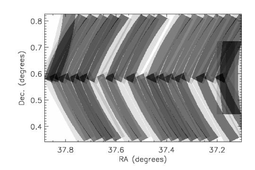
Figure 2.— Window function of spectroscopic coverage in our most complete pointing to date. We include the 32 slitmasks which have a redshift completeness $\geq 60$% in our analysis. The greyscale ranges from 0 (white) to 0.86 (black) and corresponds to the probability that a galaxy meeting our selection criteria at that position in the sky was targeted for spectroscopy. The total length of this field is 2 degrees; only the first $\sim 0.7$ degrees have been covered thus far.

Figure 3.— Redshift distribution of $\sim 5000$ galaxies observed in the first season of the DEEP2 survey, covering three separate fields for a total of 0.72 degrees². The solid line is a smoothed fit which we use to estimate our selection function, $\phi(z)$, in the redshift range $0.7<z<1.35$. The dotted and dashed lines show the normalized selection functions for the emission-line and absorption-line samples, respectively.

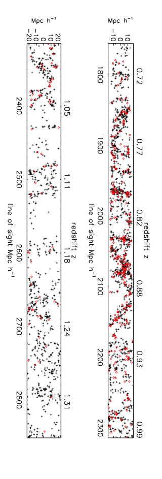
Figure 4.— Redshift-space distribution of galaxies in early DEEP2 data in our most complete field shown as a function of redshift and comoving distance along and projected distance across the line of sight, assuming a $\Lambda$CDM cosmology. We have split the sample by PCA classification: black, plus-signs show emission-line galaxies while red, diamond symbols show absorption-dominated galaxies. It is apparent that galaxies with early-type spectra are more strongly clustered.

Figure 5.— Left: Contours of the two-dimensional correlation function, $\xi(r_{p},\pi)$, smoothed with a $3\times 3$ boxcar, measured for 2219 galaxies in the redshift range $0.7<z<1.35$ in our most complete field to date. The smoothing has been applied only for the figures; it is not used in calculations. Contours levels are 0.0 (dashed), 0.25, 0.5, 0.75, 1.0 (bold), 2.0 and 5.0. Right: Contours of $\xi(r_{p},\pi)$, smoothed with a $3\times 3$ boxcar, measured for lower-redshift galaxies in our sample (solid contours) and for higher-redshift objects (dashed contours). Contours levels are 0.25, 0.5, 1.0 (bold), 2.0 and 5.0.

Figure 6.— The projected correlation function, $w_{p}(r_{p})$, for the full redshift range (top) and two redshift sub-samples (bottom). The dotted lines show power-law fits used to recover $r_{0}$ and $\gamma$ of $\xi(r)$ for each sample, as listed in Table 1. Error bars are computed from the variance across mock catalogs and are estimates of the cosmic variance.

Figure 7.— Top: $w_{p}(r_{p})$ measured for red (dashed line) and blue (solid line) subsamples, divided according to restframe $(B-R)_{0}$ color. The dotted lines show power-law fits used to estimate $r_{0}$ and $\gamma$ (see Table 1). Middle: $w_{p}(r_{p})$ measured for emission-line ($\eta>-13$, solid line) and absorption-dominated ($\eta<-13$, dashed line) subsamples classified using PCA. Bottom: $w_{p}(r_{p})$ measured for subsamples divided according to absolute magnitude, $M_{B}$, assuming $h=1$.

Figure 8.— Redshift histograms and the heavily smoothed curves used to estimate the selection functions, $\phi(z)$, for subsamples divided according to absolute magnitude, $M_{B}$, assuming $h=1$.

References

- Adelberger (1999) Adelberger, K. 1999, In ASP Conference Series Vol. 200
- Adelberger et al. (1998) Adelberger, K. L., et al. 1998, ApJ, 505, 18
- Adelberger et al. (2003) Adelberger, K. L., et al. 2003, ApJ, 584, 45
- Bardeen et al. (1986) Bardeen, J. M., et al. 1986, ApJ, 304, 15
- Benson et al. (2001) Benson, A. J., et al. 2001, MNRAS, 327, 1041
- Burles & Schlegel (2004) Burles, S., & Schlegel, D. 2004, in preparation
- Carlberg et al. (1997) Carlberg, R. G., et al. 1997, ApJ, 484, 538
- Coil et al. (2004) Coil, A. L., et al. 2004, in preparation
- Coil, Davis, & Szapudi (2001) Coil, A. L., Davis, M., & Szapudi, I. 2001, PASP, 113, 1312
- Colless et al. (2001) Colless, M., et al. 2001, MNRAS, 328, 1039
- da Costa et al. (1998) da Costa, L. N., et al. 1998, AJ, 116, 1
- Daddi et al. (2001) Daddi, E., et al. 2001, A&A, 376, 825
- Davis et al. (2002) Davis, M., et al. 2002, Proc. SPIE, 4834, 161 (astro-ph 0209419)
- Davis et al. (2004) Davis, M., et al. 2004, in preparation
- Davis & Geller (1976) Davis, M., & Geller, M. J. 1976, ApJ, 208, 13
- Davis & Huchra (1982) Davis, M., & Huchra, J. 1982, ApJ, 254, 437
- Davis & Peebles (1983) Davis, M., & Peebles, P. J. E. 1983, ApJ, 267, 465
- Davis et al. (1985) Davis, M., Efstathiou, G., Frenk, C. S., & White, S. D. M. 1985, ApJ, 292, 371
- de Lapparent, Geller, & Huchra (1988) de Lapparent, V., Geller, M. J., & Huchra, J. P. 1988, ApJ, 332, 44
- Dressler (1980) Dressler, A. 1980, ApJ, 236, 351
- Eisenstein et al. (2003) Eisenstein, D. J., et al. 2003, ApJ, 585, 694
- Faber et al. (2002) Faber, S., et al. 2002, Proc. SPIE, 4841, 1657
- Firth et al. (2002) Firth, A. E., et al. 2002, MNRAS, 332, 617
- Fisher et al. (1994) Fisher, K. B., et al. 1994, MNRAS, 267, 927
- Gerke et al. (2004) Gerke, B., et al. 2004, in preparation
- Hamilton (1993) Hamilton, A. J. S. 1993, ApJ, 417, 19
- Hawkins et al. (2003) Hawkins, E., et al. 2003, MNRAS, 346, 78
- Hermit et al. (1996) Hermit, S., et al. 1996, MNRAS, 283, 709
- Hogg, Cohen, & Blandford (2000) Hogg, D. W., Cohen, J. G., & Blandford, R. 2000, ApJ, 545, 32
- Jenkins et al. (1998) Jenkins, A., et al. 1998, ApJ, 499, 20
- Kaiser (1984) Kaiser, N. 1984, ApJ, 284, L9
- Kaiser (1987) Kaiser, N. 1987, MNRAS, 227, 1
- Kauffmann et al. (1999a) Kauffmann, G., Colberg, J. M., Diaferio, A., & White, S. D. M. 1999a, MNRAS, 303, 188
- Kauffmann et al. (1999b) Kauffmann, G., Colberg, J. M., Diaferio, A., & White, S. D. M. 1999b, MNRAS, 307, 529
- Kerscher, Szapudi, & Szalay (2000) Kerscher, M., Szapudi, I., & Szalay, A. S. 2000, ApJ, 535, L13
- Kinney et al. (1996) Kinney, A. L., et al. 1996, ApJ, 467, 38
- Lahav et al. (2002) Lahav, O., et al. 2002, MNRAS, 333, 961
- Landy & Szalay (1993) Landy, S. D., & Szalay, A. S. 1993, ApJ, 412, 64
- Le Fevre et al. (1996) Le Fevre, O., et al. 1996, ApJ, 461, 534
- Loveday et al. (1995) Loveday, J., Maddox, S. J., Efstathiou, G., & Peterson, B. A. 1995, ApJ, 442, 457
- Ma (1999) Ma, C. 1999, ApJ, 510, 32
- Madgwick et al. (2003a) Madgwick, D. S., et al. 2003a, MNRAS, 344, 847
- Madgwick et al. (2003b) Madgwick, D. S., et al. 2003b, ApJ, 599, 997
- Mo & White (1996) Mo, H. J., & White, S. D. M. 1996, MNRAS, 282, 347
- Mo, Mao, & White (1999) Mo, H. J., Mao, S., & White, S. D. M. 1999, MNRAS, 304, 175
- Moore et al. (1994) Moore, B., et al. 1994, MNRAS, 269, 742
- Newman et al. (2004) Newman, J., et al. 2004, in preparation
- Newman & Davis (2002) Newman, J. A., & Davis, M. 2002, ApJ, 564, 567
- Norberg et al. (2001) Norberg, P., et al. 2001, MNRAS, 328, 64
- Nusser & Davis (1994) Nusser, A., & Davis, M. 1994, ApJ, 421, L1
- Oke & Gunn (1983) Oke, J. B., & Gunn, J. E. 1983, ApJ, 266, 713
- Peebles (1980) Peebles, P. J. E. 1980. The Large-Scale Structure of the Universe, (Princeton, N.J., Princeton Univ. Press)
- Shectman et al. (1996) Shectman, S. A., et al. 1996, ApJ, 470, 172
- Shepherd et al. (2001) Shepherd, C. W., et al. 2001, ApJ, 560, 72
- Small et al. (1999) Small, T. A., Ma, C., Sargent, W. L. W., & Hamilton, D. 1999, ApJ, 524, 31
- Spergel et al. (2003) Spergel, D. N., et al. 2003, ApJS, 148, 175
- Tegmark & Peebles (1998) Tegmark, M., & Peebles, P. J. E. 1998, ApJ, 500, L79
- Tucker et al. (1997) Tucker, D. L., et al. 1997, MNRAS, 285, L5
- Verde et al. (2002) Verde, L., et al. 2002, MNRAS, 335, 432
- Willmer et al. (2004) Willmer, C., et al. 2004, in preparation
- Willmer, da Costa, & Pellegrini (1998) Willmer, C. N. A., da Costa, L. N., & Pellegrini, P. S. 1998, AJ, 115, 869
- Yan et al. (2003) Yan, R., et al. 2003, accepted by ApJ (astro-ph/0311230)
- York et al. (2000) York, D. G., et al. 2000, AJ, 120, 1579
- Zehavi et al. (2002) Zehavi, I., et al. 2002, ApJ, 571, 172