Constraining cosmological parameters using Sunyaev-Zel’dovich cluster surveys

Abstract

We discuss how future cluster surveys can constrain cosmological parameters with particular reference to the properties of the dark energy component responsible for the observed acceleration of the universe by probing the evolution of the surface density of clusters as a function of redshift. We explain how the abundance of clusters selected using their Sunyaev-Zel’dovich effect can be computed as a function of the observed flux and redshift taking into account observational effects due to a finite beam-size. By constructing an idealized set of simulated observations for a fiducial model, we forecast the likely constraints that might be possible for a variety of proposed surveys which are assumed to be flux limited. We find that Sunyaev-Zel’dovich cluster surveys can provide vital complementary information to those expected from surveys for supernovae. We analyse the impact of statistical and systematic uncertainties and find that they only slightly limit our ability to constrain the equation of state of the dark energy component.

I Introduction

Sunyaev and Zel’dovich [1, 2] (SZ) first noted that cosmic microwave background (CMB) photons would be re-scattered as they pass through the hot intergalactic medium in clusters of galaxies due to inverse Compton scattering. Since this process preserves the overall number of photons, one observes a decrement in CMB temperature in the Rayleigh-Jeans part of the spectrum, and a corresponding increase at high frequencies above the null frequency of 217 GHz. For a cluster of given mass, the brightness temperature depends only on the integrated pressure of the gas in the cluster along the line of sight and not on its distance since the red-shifting of the photons is exactly balanced by their higher density at the time of scattering. This not only allows the clusters to be detected at much higher redshifts than using standard optical and X-ray measurements, it also makes any detection much less susceptible to the internal dynamics of the cluster, providing a reliable method for detecting clusters in a blank field survey.

To date the SZ effect has been mapped in a small number of clusters with targeted observations using either a single dish [3, 4, 5], or an interferometer [6, 7, 8, 9, 10, 11, 12, 13, 14, 15]. In the very near future blank field surveys will be performed on dedicated instruments with arcminute resolution which should yield flux limited samples of clusters at a variety of frequencies and resolutions over large areas (see, for example, [16, 17, 18, 19, 20, 21, 22, 23, 24, 25, 26, 27, 28] and references therein). Moreover, instruments originally designed to make small scale CMB anisotropy measurements such as the Very Small Array (VSA) [29], Cosmic Background Imager (CBI) [30] and those on board the Planck Surveyor [31, 32] will also inadvertently provide information, albeit less efficiently due to their large beam sizes [33], though the Planck Surveyor can balance this disadvantage with its full sky coverage and the range of frequencies available.

The limiting mass of a survey as a function of redshift can be computed from the limiting flux assuming the cluster is virialized and, hence, that there exists a relationship between the mass of the cluster and the temperature of the gas within it. Therefore, the survey yield is a calculable function of the cosmological parameters and the process of halo formation. If we believe the physics of halo formation is understood, which in the case of cluster size halos should just involve gravitational physics, then the number of clusters as a function of redshift can be used to constrain cosmological parameters [34, 35, 36, 37, 38, 39, 40, 41, 42, 43, 44, 45]. More precisely the number of objects will depend on the comoving volume element, the angular diameter distance and the rate of growth of perturbations, all of which depend sensitively on the late-time evolution of the cosmological scale factor $a(t)$.

The study of the late-time evolution of the universe has become an important part of many observational programs ever since observations of type Ia supernovae (SNe) suggested that the expansion of the universe might be accelerating [46, 47, 48, 49]. It was found that a combined initial sample of 42 SNe with $\langle z\rangle\approx 0.6$ were much dimmer at high redshift than required by a matter dominated Einstein-de Sitter universe, with the simplest remedy being the inclusion of Einstein’s ‘greatest blunder’, the cosmological constant $\Lambda$ which gives rise to acceleration by virtue of the negative pressure associated with vacuum energy. Subsequent observations of more SNe have only strengthened this conclusion. These observations probe the magnitude-redshift relation by assuming the SNe are standard candles.

However, this is notoriously difficult to incorporate into a realistic particle physics theory since estimates of the vacuum energy, while very rarely zero, are substantially larger than the observed value. This lead to the proposal of a dynamical dark energy component with negative pressure, often called ‘Quintessence’, due to a scalar field [50, 51, 52, 53, 54, 55, 56, 57, 58, 59, 60, 61, 62]. Although this idea is not without its own problems, it provides an interesting theoretical framework to parameterize and test the idea of dark energy.

If one takes Quintessence seriously one has to accept the fact that the equation of state parameter $w_{\rm Q}=p_{\rm Q}/\rho_{\rm Q}$ is not only negative, but that it can evolve with time. There are many specific dark energy models, none of which are theoretically compelling and, therefore, in order to test them one requires some kind of parameterization of this evolution. There has been some debate in the literature about what is the best way to do this: suffice to say that it is difficult to imagine one which accurately represents every model and it is often best to tailor the parameterization to the type of observations under consideration [63, 64, 65, 66, 67, 68, 69, 70, 71]. Since the clusters under discussion here will have redshift of less than 1.5, a Taylor expansion of the form $w_{{\rm Q}}=w_{0}+w_{1}z+..\,,$ where $w_{0}$ and $w_{1}$ are constants is a sensible form to consider.

An important feature of SZ surveys, and similar observations that probe number counts, is that their dependence on the expansion rate of the universe is very different to that of SNe observations, that is, they are complimentary and, hence, can be used to break parameter degeneracies. A degeneracy between $w_{0}$ and $w_{1}$ is present for both SZ and SNe surveys. However, the shape of the likelihood contours in the $w_{0}$-$w_{1}$ plane is very different [45], allowing one to use the two together to make more substantial statements as to the nature of the dark energy.

In this paper we will discuss using the evolution of the surface density as a a function of redshift. A particular important ingredient for using number counts of clusters to constrain cosmology is the ability to measure their redshift. Ideally spectroscopic redshifts ($\Delta z\approx 0.01$) would be available for each cluster. However, it may only be possible to get photometric redshift ($\Delta z\approx 0.1)$. Moreover, at present it is difficult to estimate redshifts for objects with $z\sim 1$. The Sloan Digital Sky Survey (SDSS) [74, 75] and the Visible and Infrared Survey Telescope for Astronomy (VISTA) [76] will measure the redshift of many hundreds of thousands of galaxies and will provide this information at least to some degree. Except where explicitly stated we will use $\Delta z=0.1$ and $z_{\rm max}=1.5$, optimistically assuming techniques to find redshifts for very distant objects can be developed on a similar timescale to instruments under discussion here.

In section II we will discuss the principal cosmology dependence of the surface density of clusters on cosmology, before going on to discuss the relation between the limiting mass and the survey set up in section III. We will then perform a mock likelihood analysis for six proposed survey setups in section IV and discuss statistical and systematic uncertainties in our assumptions in section V. Note that throughout this paper algebraic relations will be expressed in natural units where $c=\hbar=k_{\rm B}=1$.

II Surface density of clusters

There exists a plethora of dark energy models none of which are particularly compelling. We will only discuss models which are minimally coupled to gravity. Since, a priori, there is no theoretical preference for any particular model we take a phenomenological approach and characterize the dark energy component by a linear evolving equation of state [66, 67, 68]

$$w_{\rm Q}=w_{0}+w_{1}z\,.$$ (1)

This is sufficient since we are only interested in the low redshift behaviour of the dark energy component and furthermore (1) approximates a wide range of dark energy models adequately at low redshifts [66, 67, 68, 69].

In order to predict the surface density of clusters of a mass limited Sunyaev-Zel’dovich survey we need to compute

$$\frac{dN}{dz}={\Delta\Omega}\frac{dV}{dzd\Omega}(z)\int\limits_{M_{\rm lim}(z)}^{\infty}\frac{dn}{dM}\,dM\,,$$ (2)

where $dV/(dzd\Omega)=[r(z)]^{2}/H$ is the comoving volume in a flat universe, with $r(z)=\int_{0}^{z}H^{-1}(z^{\prime})dz^{\prime}$ the coordinate distance, $\Delta\Omega$ is the angular sky coverage of the survey and $dn/dM$ is the comoving number density of objects with mass $M$ and redshift $z$, sometimes called the mass function. $M_{\rm lim}$ is the limiting mass, which will depend in general on the parameters of the survey. In this section, we will assume that $M_{\rm lim}$ is constant and does not depend on the cosmological parameters. In the next section, however, we will drop this assumption and model $M_{\rm lim}$ in a more realistic way for our mock likelihood analysis.

We will use the comoving number density calibrated using a series of N-body simulations performed by the VIRGO consortium [77], with

$$\frac{dn}{dM}\left(z,M\right)=-0.22\frac{\rho_{m}(t_{0})}{M\sigma_{M}}\frac{d\sigma_{M}}{dM}\exp\left\{-|0.73-\log\left[D(z)\sigma_{M}\right]|^{3.86}\right\}\,,$$ (3)

where the mass, $M$ of the object is defined to be that inside a spherical over-density of $\Delta=200$ times the critical background density, that is, $M_{200}=4\pi R_{200}^{3}200\rho_{\rm crit}(z)/3$. $D(z)$ is the growth factor normalized to have $D(0)=1$. We obtain the growth factor by solving numerically the perturbation equation for the matter fluctuations

$$\delta_{m}^{\prime\prime}+\frac{3}{2}a^{-1}\left[1-w(a)\left(1-\Omega_{\rm m}(a)\right)\right]\delta_{m}^{\prime}-\frac{3}{2}a^{-2}\Omega_{\rm m}(a)\delta_{m}=0\,,$$ (4)

where the prime denotes the derivative with respect to the scale factor $a$ and we choose our initial conditions to be setup in the matter dominated era with $\delta_{m}(a_{i})=a_{i}$ and $\delta_{m}^{\prime}(a_{i})=1$, where $z_{i}=30$ is sufficient. The growth factor is then given by $D(z)=\delta_{m}(z)/\delta_{m}(z=0)$. Furthermore, $\rho_{m}(t_{0})$ is the present day matter density, $\Omega_{\rm m}(a)=\rho_{m}(a)/\rho_{\rm crit}(a)$ is the matter density in units of the critical density and $\sigma_{M}$ is the over-density with mass $M$ today, where

$$\sigma_{R}^{2}=\int_{0}^{\infty}W^{2}(kR)\Delta^{2}(k)\frac{dk}{k}$$ (5)

and $M=4\pi\rho_{m}(t_{0})R^{3}/3$. The window function in (5) is that of a spherical top hat with $W(x)=3(\sin(x)/x^{3}-\cos(x)/x^{2})$.

The final missing ingredient is the linear power spectrum $P(k)$, where $\Delta^{2}(k)=4\pi k^{3}P(k)$. We define the transfer function $T(k,z)$ via $P(k)=Ak^{n}[T(k,z)]^{2}$, where $n$ is the spectral index. CMBFAST [78] is used to compute the shape of the transfer functions in $k$ space, where it is sufficient to approximate the perturbations of a dark energy model with the corresponding $\Lambda$CDM model, since clustering on small scales is not affected by the presence of a dark energy component. We fix the baryonic component to have $\Omega_{\rm b}h^{2}=0.019$ in agreement with Big Bang Nucleosynthesis constraints [79, 80]. To normalize the power spectrum, we use $\sigma_{8}$, the over-density in a spherical region of $8h^{-1}{\rm Mpc}$, which is traditionally used to quantify the amplitude of the power spectrum on small scales.

For our fiducial model we choose $\sigma_{8}=0.9$ as suggested by recent CMB measurements [81]. Note that this value is higher than the one inferred from recent X-ray measurements [82, 83, 84]. One might think that this discrepancy is not very worrying since $\sigma_{8}$ is a parameter which we are trying to determine. However, since the number of objects found in a given survey is very sensitive to $\sigma_{8}$ and the statistics is Poisson distributed, using a much smaller value, $\sigma_{8}=0.7$ say, would substantially weaken our conclusions. Also we assume that the universe is flat and $H_{0}=72\,{\rm km}\,{\rm sec}^{-1}{\rm Mpc}^{-1}$ [85], $\Omega_{m}(t_{0})=0.3$ and a spectral index $n=1$ [86, 87, 88]. For the dark energy equation of state parameters we choose $w_{0}=-0.8$ and $w_{1}=0.3$ which is allowed by current data  [90, 91, 86, 87] and is compatible with an interesting Supergravity related Quintessence model [61, 69].

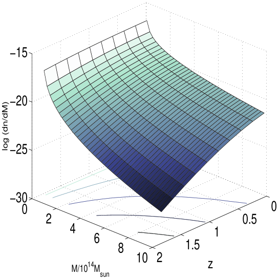
FIG. 1.: The comoving mass density $dn/dM$ in units of $[{\rm Mpc}^{3}M_{\odot}]^{-1}$ from simulations of the VIRGO consortium [77] using a $\Lambda$CDM cosmology. The lines on the base of the plot represent contours of constant $dn/dM$.

In Fig. 1 we show the comoving mass density for a $\Lambda$CDM cosmology (w=-1). The rapid decrease for large cluster masses and large redshifts is clearly visible and we expect a low number of clusters in these ranges. This choice of comoving number density is similar to the usual Press-Schechter (PS) formalism [92]. However, the PS approach shows some significant differences from the observed and simulated comoving number density. The simulations show less low and an increased number of high mass clusters (see also Fig. 13) compared to the PS prescription. A much better fit is achieved from using PS if one assumes an aspherical collapse [93, 94, 41]. Also note that the mass function has an uncertainty [41, 94, 95, 77, 96] and we will come to this problem when we discuss systematic errors in section V.

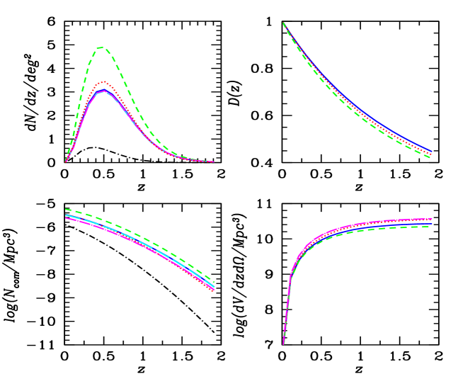
FIG. 2.: In the top left we show the surface density of clusters above a mass limit of $M_{\rm lim}=2.35\times 10^{14}M_{\odot}$ as a function of redshift. The top right is the normalized growth factor $D(z)$, the lower left the comoving number of clusters $N_{\rm com}(z)$ and the lower right is the volume element $dV/(dzd\Omega$). The solid line is the fiducial cosmology (see text), the dotted line a $\Lambda$CDM cosmology, the short dashed line is for $\Omega_{\rm m}(t_{0})=0.4$, the long dashed line for $n=0.9$ (almost underneath the solid line), the dot - short dash line for $\sigma_{8}=0.72$ and the dot - long dash line for $H_{0}=65\,{\rm km}\,{\rm sec}^{-1}{\rm Mpc}^{-1}$.

In the following we will discuss the dependence on cosmology of the number of objects per square degree above a given mass limit $M_{\rm lim}=2.35\times 10^{14}M_{\odot}$. We will see in section III that $M_{\rm lim}=M_{\rm lim}(z)$, but using a fixed limiting mass should provide some intuitive information. In Fig. 2 we present the surface density of clusters (top left) and its constituents, the comoving number density, $N_{\rm com}=\int_{M_{\rm lim}(z)}^{\infty}\frac{dn}{dM}\,dM$, (lower left), the growth factor (top right) and the volume (lower right). As a base for comparison we use the fiducial cosmology described above and then change subsequently one parameter. As expected the strongest dependence is on $\sigma_{8}$ and $\Omega_{m}(t_{0})$. However, we see a weak, but nonetheless significant dependence on the equation of state parameters $w_{0}$ and $w_{1}$. The dependence on the spectral index $n$ is very weak and hence we fix $n=1.0$ in the subsequent analysis. We also see that the strongest dependence must come from the linear growth factor (upper right panel), since minute changes lead to significant changes in the surface density. This is most obvious from the change in the $\Omega_{\rm m}$ (dashed line), where the volume element (lower right panel) would predict a lower number of clusters, which is balanced by the faster growing linear perturbations (top right). This is clear, since the dependence of the surface density on the growth factor is exponential (Eqn. 3).

III The limiting mass

In the previous section we assumed that the mass limit of the survey is constant. However, in a realistic observing situation the survey is limited by the flux and not mass. Hence, we need a relation between the flux limit $S_{\rm lim}$ and the mass limit $M_{\rm lim}$. We should note that, contrary to what is often explicitly stated or implied in the literature, the surveys are not mass limited in the sense that there is single limiting mass which applies across a wide range of redshifts. If one were to use a fixed limiting mass, one would be either forced to throw out many objects in order to make the survey complete to some high threshold, or put up with lack of completeness at both low and high redshifts with a smaller threshold. Here, we will discuss how to compute the limiting mass by first making the extreme, and generally incorrect assumption, that the cluster is point-like in the telescope beam. We will then extend our results to clusters which are resolved. A more detailed discussion of this problem can be found in the relevant section of the companion paper [98]

A Principal dependence on cosmology

We first construct the relation between the virial mass and flux limit of the survey assuming that the source is point-like in the telescope beam. The total flux density and the brightness temperature are related by [1, 2, 97]

$$S_{\nu}=2\nu^{2}\Delta Tf(x)=2\nu^{2}T_{\rm CMB}f(x)Y\,,$$ (6)

with $f(x)=x^{2}e^{x}g(x)/(e^{x}-1)^{2}$ and $g(x)=x/{\rm tanh}(x/2)-4$, where $x=2\pi\nu/T_{\rm CMB}$ is the dimensionless frequency. The $Y$ parameter is given by the integrated y-distortion $Y=\int d\Omega y(\theta)$, with

$$y(\theta)={\sigma_{\rm T}\over m_{\rm e}}\int dl\,n_{\rm e}\,T_{\rm e}={\langle T_{\rm e}\rangle_{n}\over m_{\rm e}}\tau_{\rm e}(\theta)\,,$$ (7)

the line of sight integral over the gas pressure in the cluster. The Thomson scattering cross section is $\sigma_{\rm T}$ and $m_{\rm e}$ is the electron mass. We have introduced the electron density weighted average temperature $\left<T_{\rm e}\right>_{n}=\int dl\,n_{\rm e}T_{\rm e}/\int dl\,n_{\rm e}$, and $\tau_{\rm e}(\theta)=\sigma_{\rm T}\int dl\,n_{\rm e}$ the optical depth.

It is conventional to normalize the optical depth in terms of the virial mass of the cluster using

$${M_{\rm vir}f_{\rm gas}\over\mu_{\rm e}m_{\rm p}}=\int d^{3}r\,n_{\rm e}({\bf r})=d_{A}^{2}\int d\Omega dln_{\rm e}\,,$$ (8)

from which one can deduce that

$$\tau_{\rm e}(0)=\sigma_{\rm T}{1\over d_{\rm A}^{2}}{f_{\rm gas}M_{\rm vir}\over\mu_{\rm e}m_{\rm p}}\left(\int\zeta(\theta)d\Omega\right)^{-1}\,,$$ (9)

where $\tau_{\rm e}(\theta)=\tau_{\rm e}(0)\zeta(\theta)$, $f_{\rm gas}$ is the intra cluster gas fraction, which we choose $f_{\rm gas}=0.12$ throughout this paper [99], $\mu_{\rm e}=1.143$ the mean mass per electron and $m_{\rm p}$ the proton mass. In the general the profile $\zeta(\theta)$ will depend on the virial radius $R_{\rm vir}$ and redshift $z$ via the angular diameter distance, which for a flat universe is given by $d_{A}(z)=(1+z)^{-1}\int_{0}^{z}H^{-1}(z^{\prime})\,dz^{\prime}$. Using this normalization, it is easy to see from this that the flux density is given by

$$S_{\nu}={2\nu^{2}T_{\rm CMB}\langle T_{\rm e}\rangle_{n}\over m_{\rm e}}{f_{\rm gas}M_{\rm vir}\over\mu_{\rm e}m_{\rm p}}{1\over d_{\rm A}^{2}}\sigma_{\rm T}f(x)\,,$$ (10)

In order to solve (10) for the mass for a given flux limit, we need to know the relation between mass $M_{\rm vir}$ and the cluster temperature $\langle T_{\rm e}\rangle_{n}$. We assume that clusters are virialized objects which are in thermal equilibrium. This assumption seems to be confirmed by recent X-ray observations [84], though it is expected that due to ongoing mergers and heat input, this assumption does not hold for high redshifts [100]; an issue we will discuss in section V. If we assume that the cluster is virialized the kinetic energy at virialization $E^{\rm kin}_{\rm vir}$ is given by

$$E^{\rm kin}_{\rm vir}=-\frac{1}{2}U_{G}+U_{{\rm Q}}\,,$$ (11)

with $U_{G}=-3GM_{\rm vir}^{2}/(5R_{\rm vir})$ the potential energy due to the gravity of the matter. By integrating $\epsilon_{\rm Q}=\rho_{\rm Q}+3p_{\rm Q}$ over the sphere, with equation of state factor $w$ and assuming that $\rho_{{\rm Q}}$ is smooth on cluster scales, we obtain the general expression for the potential energy

$$U_{Q}=\frac{1+3w}{10}4\pi G\rho_{{\rm Q}}(a)R_{\rm vir}^{2}M_{\rm vir}\,.$$ (12)

Note that (12) is the generalization of the well known result for a cosmological constant [101], and is different to the form used in [40]. We can relate the virial mass of the cluster to the virial radius, by assuming spherical symmetry $M_{\rm vir}=4\pi R_{\rm vir}^{3}\rho_{\rm cluster}/3$, where $\rho_{\rm cluster}$ is the mean density of the cluster. The mean kinetic energy $E^{\rm kin}_{\rm vir}=M_{\rm vir}\left<V_{\rm vir}^{2}\right>/2$ is given in terms of the root mean square of the velocity dispersion of the cluster. If the cluster is in thermal equilibrium, the virialization temperature is given by [102, 103, 104]

$$\langle T_{\rm e}\rangle_{n}=\frac{1}{3}\mu m_{\rm p}\langle V_{\rm vir}^{2}\rangle\,,$$ (13)

with $\mu=0.59$ the mean mass per particle. Hence, we deduce that

$$\frac{M_{\rm vir}}{10^{15}h^{-1}M_{\odot}}=\left(\frac{\left<T_{\rm e}\right>_{n}}{T_{*}}\right)^{3/2}\left(\Delta_{c}E(z)^{2}\right)^{-1/2}\left[1+\left(1+3w\right)\frac{\Omega_{\rm Q}(z)}{\Delta_{c}}\right]^{-3/2}\,,$$ (14)

where $T_{*}$ is a normalization factor which can be deduced to be $T_{*}\approx 0.5$ under the assumption that the process of virialization only involves gravitational heating . Both simulations [103, 41] and observations appear to be somewhat inconsistent with this value. For our subsequent analysis we choose $T_{*}=1.6$ and we will come back to this in section V A. Note that we have expressed the mean cluster density in terms of the over-density $\Delta_{c}$ of the cluster at virialization, with $\rho_{\rm cluster}=\Delta_{c}\rho_{\rm crit}$.

We can solve numerically for the over-density at virialization by applying the spherical collapse model  [105, 106, 38, 40]. We follow essentially the discussion in [40] where the background cosmology is described by the Friedman equation

$$\left(\frac{{\dot{a}}}{a}\right)^{2}=\frac{8\pi G}{3}\left(\rho_{m}+\rho_{Q}\right)\,.$$ (15)

and the collapsing cluster of radius $R$ by

$$\frac{{\ddot{R}}}{R}=-{4\pi G\over 3}\left[\left(1+3w\right)\rho_{Q}+\rho_{\rm cluster}\right]\,.$$ (16)

As before, we make the standard assumption that the dark energy component does not clump on the relevant scales. We can solve this coupled system numerically and obtain the density of the cluster at turnaround $t=t_{\rm ta}$, $\rho_{\rm cluster}=\zeta_{\rm ta}\rho_{\rm m}$, and obtain a best fit for the over-density

$$\zeta_{\rm ta}(z_{\rm ta})\approx\left(\frac{3\pi}{4}\right)^{2}\Omega_{m}(z_{\rm ta})^{-0.79+0.26\Omega_{m}(z_{\rm ta})-0.08(w_{0}-w_{1})-0.21w_{1}(1+z_{\rm ta})}\,.$$ (17)

We can then scale this result to the time of virialization, $t=t_{\rm v}=2t_{\rm ta}$, with

$$\Delta_{c}(z_{\rm v})=\zeta_{\rm ta}(z_{\rm ta})\Omega_{\rm m}(z)\left(\frac{R_{\rm ta}}{R_{\rm vir}}\right)^{3}\left(\frac{1+z_{\rm ta}}{1+z_{\rm v}}\right)^{3}\,,$$ (18)

where we have introduced

$$\frac{R_{\rm vir}}{R_{\rm ta}}\approx\frac{1-\eta_{\rm v}/2}{2+\eta_{\rm t}-3/2\eta_{\rm v}}\,,$$ (19)

the ratio of the radius at virialization (or collapse) of the cluster to the radius at turn around with

$$\eta_{\rm t} = -\left[1+3w(z_{\rm ta})\right]\frac{\Omega_{\rm Q}(z_{\rm ta})}{\zeta_{\rm ta}\Omega_{m}(z_{\rm ta})}\,,$$ (20)

$$\eta_{\rm v} = -\left[1+3w(z_{\rm v})\right]\frac{\Omega_{\rm Q}(z_{\rm v})}{\zeta_{\rm ta}\Omega_{m}(z_{\rm v})}\left(\frac{1+z_{\rm v}}{1+z_{\rm ta}}\right)^{3}\,.$$ (21)

Note that again these expressions differ from [40] because of the generalized potential for the dark energy component in (12). We have now all the necessary ingredients to calculate the virial mass of a cluster for a given Sunyaev-Zel’dovich flux decrement. However in order to calculate the limiting mass in (3) we need to transform the virial mass from an over-density of $\Delta_{c}$ to an over density of $\Delta=200$. In order to do this we assume that the matter in the cluster is distributed according to a Navarro-Frenk-White (NFW) profile [107], with a concentration parameter $c=5$. This allows us to rescale the cluster mass from $M_{\rm vir}$ to $M_{200}$.

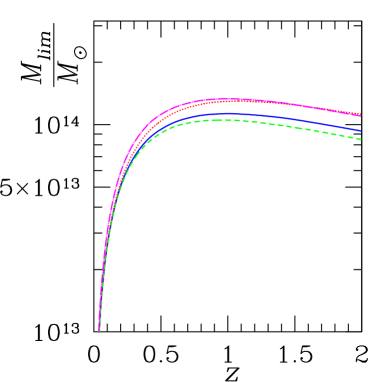
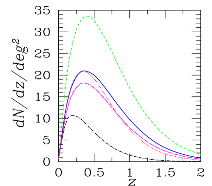
FIG. 3.: The limiting mass (left) and surface density of clusters (right) in the point source approximation for a survey with limiting flux density $S_{\rm lim}=4.4\,{\rm mJy}$ and frequency $\nu=150\,{\rm GHz}$. The different lines correspond to different cosmological parameters with the key the same as in Fig. 2.

In Fig. 3 we illustrate the limiting mass and redshift distribution of clusters using the point source approximation for the same cosmologies as in Fig. 2. First, notice that the limiting mass depends on the cosmological parameters. As well as the standard dependence on $H_{0}$, we see dependence on $\Omega_{\rm m}$ and $w_{0}$ which would be ignored by assuming that the limiting mass is constant. Note, that the dependence of $M_{\rm lim}$ on $w_{0}$ now lowers the overall number of clusters (dotted line), balancing the slight increase of the number of clusters for the $\Lambda$CDM universe, compared to the fiducial model in the case of a fixed limiting mass (see Fig. 2). For an increasing $\Omega_{\rm m}$ the limiting mass is decreasing resulting in an even more enhanced number of clusters compared to the fiducial model. Moreover, in this approximation the limiting mass goes to zero at low redshifts. Although this will be seen to be unphysical when telescope beams are small, it will be a good approximation when the beam is large. The dependence of the limiting mass on the cosmological parameters feeds into the predictions for $dN/dz$, but the effects of parameters such as $\sigma_{8}$ and $n$ is unchanged from that for a constant limiting mass.

B Extended clusters and survey beam

So far we have not accounted for the possibility of clusters being extended objects within the telescope beam which could lead to a loss of flux. If there is a beam $B(\theta)$ present, integrated y-distortion in (6) becomes [108]

$$Y=\int d\Omega\,y(\theta)\quad\to\quad Y=\frac{\int d\Omega\,B(\theta)y(\theta)}{\int d\Omega B(\theta)}\,,$$ (22)

where we assume a Gaussian profile of the beam, with $B(\theta)=\exp[-\theta^{2}/(2\sigma_{b}^{2})]$ and $\sigma_{b}$ is related to the full-width-half-maximum (FWHM) of the beam by $\sigma_{b}=\theta_{\rm FWHM}/\sqrt{8\ln 2}$. The equation for the observed flux for a beam directly over the centre of the cluster is then [98]

$$S_{\nu}={2\nu^{2}T_{\rm CMB}\langle T_{\rm e}\rangle_{n}\over m_{\rm e}}{f_{\rm gas}M_{\rm vir}\over\mu_{\rm e}m_{\rm p}}{1\over d_{\rm A}^{2}}\sigma_{\rm T}f(x){\cal I}(B,\zeta)\,,$$ (23)

with

$${\cal I}(B,\zeta)={\int d\Omega B(\theta)\zeta(\theta)\over\int d\Omega B(\theta)\int d\Omega\zeta(\theta)}\,.$$ (24)

In general this function will depend on $M_{\rm vir}$ via $R_{\rm vir}$, so a simple analytical solution for $M_{\rm vir}$ in terms of $S_{\rm lim}$ and $z$ is not possible and therefore we must solve (23) numerically using the Newton-Raphson method. The expression (23) is the flux in a single beam, however, if the cluster is larger than one beam area , beams can be combined with a resultant increase in the noise; a process often known as beam smoothing. The optimum number of beams is given by

$$N_{\rm b}=\frac{\int d\Omega\,\zeta(\theta)}{\int d\Omega\,B(\theta)}\,,$$ (25)

as discussed in [98]. In reality $N_{\rm b}$ must be an integer, but we will allow it here to take any value greater than one. It was shown in [98] that this does not unduly exaggerate the predicted number of clusters detected.

In most situations there will be a limit to the extent to which one can beam smooth, for example, due to the primary CMB anisotropy. In the subsequent discussion we will assume that $\theta_{\rm FWHM}^{\rm max}=20^{\prime}$. Note that for multi-frequency observations like Planck it may be possible to effectively filter out the SZ signal due its distinct spectral signature. This in principle would allow to combine even more pixels, however we do not include this effect in our analysis and we do not expect it to be significant, since it will be important only for objects at low redshifts.

We assume that the cluster is in hydrostatic equilibrium and can be described by a truncated isothermal $\beta$-model [109, 110], with an electron density distribution of

$$n_{\rm e}(r)=\left\{\begin{array}[]{c@{\qquad}l}n_{0}\left(1+\frac{r^{2}}{R_{\rm c}^{2}}\right)^{-\frac{3\beta}{2}}&r<R_{\rm vir}\\ 0&r\geq R_{\rm vir}\end{array}\,,\right.$$ (26)

where $R_{\rm c}$ is the core radius of the cluster defined in terms of the virial radius $R_{\rm c}=R_{\rm vir}/\alpha$. The projected profile function is then

$$\zeta(\theta)=\left(1+\frac{\theta^{2}}{\theta_{c}^{2}}\right)^{\frac{1}{2}-\frac{3}{2}\beta}\,\frac{J\left[\left(\frac{\alpha^{2}-\theta^{2}/\theta_{c}^{2}}{1+\theta^{2}/\theta_{c}^{2}}\right)^{1/2},\beta\right]}{J(\alpha,\beta)}\,,$$ (27)

where $J(a,b)=\int_{0}^{a}(1+x^{2})^{-3b/2}\,dx$ and $\theta_{\rm c}=R_{\rm c}/d_{\rm A}$. For the purposes of our discussion we will assume that $\beta=2/3$ and $\alpha=10$ [108], in which case

$$J(a,2/3)=\tan^{-1}(a)\,.$$ (28)

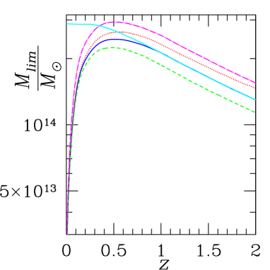
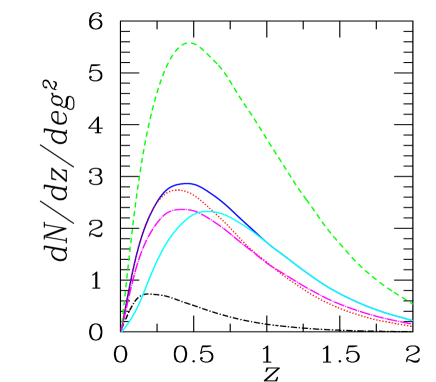
FIG. 4.: The limiting mass (left) and surface density of clusters (right) for a survey with limiting flux $S_{\rm lim}=2.62\,{\rm mJy}$ per beam, a frequency $\nu=150\,{\rm GHz}$ and a beam width of $\theta_{\rm FWHM}=1.3^{\prime}$ for an optimal combination of pixels up to a angular size of $\theta_{\rm FWHM}^{\rm max}=20^{\prime}$. The different lines correspond to different cosmological parameters with the key the same as in Fig. 2. The light solid line corresponds to the no beam smoothing case, when we fix $N_{\rm b}=1$.

Fig. 4 illustrates the limiting mass and redshift distribution of clusters if we use a beam of $\theta_{\rm FWHM}=1.3^{\prime}$. The cosmology dependence is very similar to the point source approximation. We also include the result if we allow no beam smoothing (light, solid line). We see that below a redshift of $z=1$ the possibility of beam smoothing becomes an important feature. With $\theta_{\rm FWHM}=1.3^{\prime}$ and $\theta_{\rm FWHM}^{\rm max}=20^{\prime}$ it is possible to combine up to $60$ beams, which leads for $z=0.4$ to a limiting mass which is $5\times 10^{13}{\rm M}_{\odot}$ lower than without smoothing. Furthermore we note that the limiting mass is not dropping to zero as it is the case in the point source approximation. For the surface density we see how combining the pixels improves the situation in the low redshift region. We have now all the ingredients to perform a likelihood analysis for different types of the surveys, which we will discuss in the next section.

IV Likelihood Analysis of Proposed Surveys

A Proposed surveys

In order to be able to make some firm statements as to the extent to which one might be able to constrain cosmological parameters we have to specify the flux limit $S_{\rm lim}$, the angular coverage $\Delta\Omega$, the frequency of observation $\nu$ and the beam size $\theta_{\rm FWHM}$ of the survey. This is a large parameter space and it would be prohibitive to explore it fully. Hence, we have decided to devote our attention to modelling six instruments which have been proposed and which cover a wide range of possibilities. They are the VSA [29], BOLOCAM [16, 17], the Arcminute Microkelvin Imager (AMI) [18, 19], the One-Centimetre Receiver Array (OCRA) [24], the Planck Surveyor Satellite and the South Pole Telescope (SPT) [25, 26, 111]. We have not specifically include the Sunyaev-Zel’dovich Array (SZA) [20, 21, 22] and the Array for Microwave Background Anisotropy (AMIBA) [23] in our analysis since they are likely to of very similar sensitivity to AMI. Other experiments are proposed, but we do not have sufficient information to include them in our calculations. We should caution the reader that these instruments use a wide range of different techniques, have/will cost wildly different amounts of money and will become operational over a wide range of timescales. It is not our intention to discuss the merits of particular experiments rather give a picture of the likely progression of the subject.

The values which we have chosen to represent each instrument are presented in Table I. The particular values for $S_{\rm lim}$ and $\Delta\Omega$ use a quoted instantaneous sensitivity (either for the whole instrument or individual beams) and the optimal depth of the survey using the procedure discussed in [98]. The angular coverage can then be computed from the instantaneous field of view and assuming one full year integration time. Very different results would be achieved by trading off sensitivity for area according to $S_{\rm lim}/\sqrt{\Delta\Omega}$. However, any changes from the quoted values would lead to fewer objects being found and would, therefore, be likely to lead to weaker constraints on cosmological parameters. This statement is only true for our particular modelling of the distribution of clusters.

It is worth making some comments on how we have done this for each of the different instruments:

VSA : A 14-element interferometer based on Tenerife. We use the specification for a proposed upgrade which should have an instantaneous sensitivity of $I=0.5\,{\rm Jy}\,{\rm sec}^{1/2}$ on a field of view of $\Omega_{\rm FOV}=1\,{\rm deg}^{2}$.

BOLOCAM : This instrument has 144 instantaneous beams and is being used on the 8m telescope at the Caltech Sub-millimetre Observatory on Hawaii. We estimate $\theta_{\rm FWHM}=0.8^{\prime}$ at 150 GHz and each of the beams has $I=35\,{\rm mJy}\,{\rm sec}^{1/2}$. Atmospheric emission could well require some beam switching, but for our calculations we assume that all 144 beams measure the sky providing an instantaneous field of view $\Omega_{\rm FOV}=0.025\,{\rm deg}^{2}$.

AMI : Consists of the eight 13m dishes of the Ryle Telescope and a new array of ten 3.7m antennas. It should have $\sqrt{\Omega_{\rm FOV}}=21^{\prime}$ and $I=20\,{\rm mJy}\,{\rm sec}^{1/2}$. The extra resolution provided by the Ryle baselines should allow for an investigation of the potential problem of radio point sources inside the clusters which would dilute the signal at low frequencies.

OCRA : Currently funded is a 10 beam system which will use 30 GHz receivers similar to those developed for the Planck LFI system. This will be mounted on the 32m telescope at Torun in Poland. Since the atmosphere is likely to be significant at this location the receivers will be used in pairs each with $I=5\,{\rm mJy}\,{\rm sec}^{1/2}$. We present results for a proposed 100 beam system which should have $\Omega_{\rm FOV}=0.034{\rm deg^{2}}$.

PLANCK Surveyor : Here, we use the likely sensitivity for 2 whole scans of the sky which should take 14 months for the 100 GHz channel on the HFI instrument. We conservatively assume that it should be possible to extract the SZ signal over 1/2 of the sky. We have not attempted to optimize the yield of this survey since the satellite will cover the whole sky.

SPT : This is an ambitious project to build a 10m telescope at the South Pole and mount on it a 1000 element bolometric array. It should be possible for such an array to achieve $S_{\rm lim}=5\,{\rm mJy}$ on $\Delta\Omega=4000\,{\rm deg}^{2}$ [111]

The number of clusters we predict for the fiducial cosmology and the setups of Table I are $\approx 60$ for VSA, $\approx 400$ for BOLOCAM, $\approx 170$ for AMI, $\approx 460$ for OCRA, $\approx 4500$ for SPT and $\approx 5200$ for the Planck surveyor.

	$S_{\rm lim}\;[{\rm mJy}]$	$\nu\;[{\rm GHz}]$	$\theta_{\rm fwhm}$	$\Delta\Omega\;[{\rm deg}^{2}]$
VSA	$5.75$	$30$	$8.0^{\prime}$	$300$
BOLOCAM	$1.64$	$150$	$0.8^{\prime}$	$130$
AMI	$0.58$	$15$	$4.5^{\prime}$	$230$
OCRA	$0.30$	$30$	$1.1^{\prime}$	$140$
Planck	$41.5$	$100$	$9.2^{\prime}$	$20600$
SPT	$2.62$	$150$	$1.3^{\prime}$	$1430$

TABLE I.: The experimental parameters for the six different SZ surveys assuming approximately one year integration time.

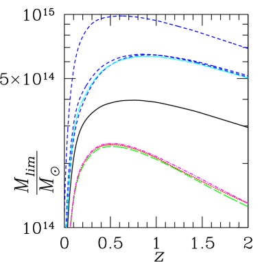
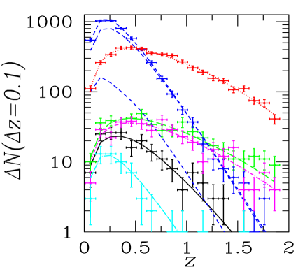
FIG. 5.: Limiting mass (left) and number of clusters (right) in redshift bins of $\Delta z=0.1$ for the different experimental setups from Table I. The dot - short dash line is for BOLOCAM, the dot - long dash line for VSA, the solid line is for the AMI survey, the long dashed line for OCRA, short dashed lines for the 100, 143 and 353 GHz channels of the Planck Surveyor (note that we only use the 100 GHz channel in the further analysis since it predicts the largest number of clusters) and the dotted line for SPT. The data points are from a randomly generated sample assuming Poisson errors. Note that we have approximated the errorbars in the plot with a Gaussian distribution of width $\sqrt{\Delta N}$. The plots are all for the fiducial cosmology.

In Fig. 5, we present the computed mass limit of the proposed surveys. Due to the fact that we have optimized the survey yield, instruments with similar beam sizes have similar limiting masses, that is SPT, OCRA and BOLOCAM have the lowest limiting masses and are approximately the same, as are VSA and Planck which have the highest limiting mass because of their large beams and low sensitivity per beam. On the right in Fig. 5 we show the surface density of clusters in bins of $\Delta z=0.1$. VSA should find a handful of clusters in each bin while AMI could discover up to $\approx$ 20 clusters in some bins around the peak near $z=0.3$. BOLOCAM and OCRA will observe a few tens of clusters in the redshift bins around the peak region and many more at high redshifts than Planck. This is is due to the small beam size. Although SPT will observe fewer clusters than Planck, in the region above redshift $z=0.5$ the cluster yield of SPT is far larger than the one from Planck, again due to its comparably small beam.

B Poisson statistics

In the following we will discuss the ability of these experiments to constrain cosmological parameters. Therefore we need to define a statistic to treat this problem quantitatively. We assume that the measurement is dominated by Poisson statistics. If we measure $N_{{\rm bin},i}$ clusters in a particular redshift bin $z_{i}$ the overall probability to observe $\{n_{i}\}$ clusters in $N_{\rm dat}$ bins is then

$$p\left(\left\{n_{i}\right\}|\left\{N_{{\rm bin},i}\right\}\right)=\prod_{i=1}^{N_{\rm dat}}\frac{N_{{\rm bin},i}^{n_{i}}}{n_{i}!}e^{-N_{{\rm bin},i}}\,.$$ (29)

We would like to test how probable it is that a given theory fits our measurement $\{N_{{\rm bin},i},z_{i}\}$. Therefore, we have to calculate $p\left(\left\{N^{\rm theory}_{\rm bin}(z_{i})\right\}|\left\{N_{{\rm bin},i}\right\}\right)$, with $N^{\rm theory}_{\rm bin}(z_{i})=\int_{z_{i}-\Delta z/2}^{z_{i}+\Delta z/2}dN/dz(z)\,dz$. We can build a log-likelihood statistic by defining

$$C=-2\ln p=-2\sum_{i=1}^{N_{\rm dat}}N^{\rm theory}_{\rm bin}(z_{i})\ln N_{{\rm bin},i}-N_{{\rm bin},i}-\ln N^{\rm theory}_{\rm bin}(z_{i})\,,$$ (30)

which is known in the literature as Cash C statistic [112]. We will sample the log-likelihood function in (30) around our fiducial cosmology, where we assume that we can get redshifts out to $z_{\rm max}=1.5$ with an accuracy of $\Delta z=0.1$. This should be feasible with photometric redshifts from instruments like the SDSS and VISTA [74, 75, 76]. For an efficient way of sampling we adopt a Markov chain Monte Carlo sampling method [113, 114, 87], where we typically compute half a million of samples to achieve convergence. For the likelihood scanning we vary $H_{0}$, $\Omega_{\rm m}$, $\sigma_{8}$, $w_{0}$ and $w_{1}$ and keep the other parameters fixed. In order to speed up the likelihood calculation we also approximate the calculation of $\sigma(R)$ in (5) by the expressions given in [115, 116].

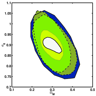
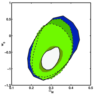
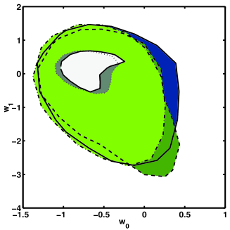
FIG. 6.: $1-\sigma$ joint likelihood contours marginalized over all the other parameters with a prior on $H_{0}=72\pm 8\,{\rm km}\,{\rm sec}^{-1}\,{\rm Mpc}^{-1}$. From outside in the contours correspond to AMI, BOLOCAM, OCRA, SPT and Planck. Note that VSA yields weaker constraints than AMI and has been omitted.

C Mock likelihood analysis

In Fig. 6 we present the joint $1-\sigma$ likelihood contours for the mock surveys. We have marginalized over all the other parameters and the only prior assumption made was that $H_{0}=72\pm 8\,{\rm km}{\rm sec}^{-1}{\rm Mpc}^{-1}$ as suggested by the Hubble Space Telescope Key Project [85]. Note that we include a larger number of parameters in our analysis than in previous analyses which naturally tends to increase the size of the errorbars. It is clear that the results from VSA, BOLOCAM, AMI and OCRA are unlikely to improve on current constraints on the cosmological parameters, but that they will provide extra independent, complementary information which can be used in conjunction with, for example, that from the primary CMB. It is possible that these surveys could be used in conjunction with X-ray or weak lensing observations of clusters to probe the gas physics of clusters and as well as to constrain cosmological parameters, providing further insight for future more powerful surveys.

Our analysis shows that Planck and SPT are likely to yield tight constraints on $\sigma_{8}$ and $\Omega_{m}$. They will be also able to start to constrain the equation of state parameters. However,it seems that the surface density of clusters alone will not be able to distinguish the fiducial model from a $\Lambda$CDM cosmology. In order to achieve tighter constraints on the equation of state it will necessary to use additional complementary information from SNe observations [117], baryon mass fraction measurements [88] or other cluster abundance measurements [84]. In the subsequent discussion we will focus on the SPT survey.

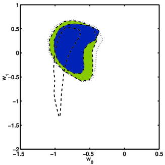
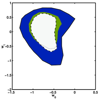
FIG. 7.: The $1-\sigma$ joint likelihood in the $w_{1}-w_{0}$ plane for the SPT survey. On the left, standard SPT (dotted), with a prior on $\Omega_{m}=0.3\pm 0.04$ (dashed filled contour) and with prior on $\Omega_{\rm m}=0.3\pm 0.02$ and $\sigma_{8}=0.9\pm 0.01$ (inner dot-dashed filled contour). The dashed line is for the Supernovae Acceleration Probe – SNAP. On the right, $z_{\rm max}=1.0$ (solid), standard SPT (dotted), SPT with $\Delta z=0.01$ (dot-dashed).

In Fig. 7, we investigate the use of prior information on $\Omega_{\rm m}$ and $\sigma_{8}$. First, we include an uncertainty of $\Delta\Omega_{\rm m}=\pm 0.04$ (solid). This accuracy has been already achieved for measurements of the baryonic gas fraction in clusters using X-ray techniques [88]. It was established that this uncertainty is relatively insensitive to the inclusion of a dark energy component and hence we use it without modification [89]. We see that such a prior does not significantly improve our ability to constrain the dark energy parameters. In order to improve on this, we have also put very tight priors on $\Omega_{\rm m}$ and $\sigma_{8}$, with $\Delta\Omega_{\rm m}=0.02$ and $\Delta\sigma_{8}=\pm 0.01$ (dot-dashed); a level of constraint which could be possible using X-ray and lensing observations [84]. This serves illustrate how sensitive the cluster abundance measurement is to the value of $\sigma_{8}$ since the constraint on the dark energy is substantially improved. If there is a tight prior on $\sigma_{8}$ then other cosmological parameters can be tightly constrained using SZ surveys.

The dashed open contour is the $1-\sigma$ likelihood for the proposed SNAP survey. We assumed for this analysis that SNAP will discover about 2000 SNe out to redshift of $z=1.7$ [68, 69]. We see that SZ surveys provide valuable complementary information to SNe surveys. The SNe seem to constrain the constant part of the equation of state, $w_{0}$, much more tightly than the evolving part $w_{1}$, while SZ clusters appear to constrain both parameters equally. This is because the surface density of clusters essentially constrains cosmological parameters via the linear growth factor $D(z)$ and the volume element $dV/(dzd\Omega)$, while SNe constrains on the magnitude-redshift relation. As a note of caution we find that even using SPT with the tightest priors as well as SNAP one cannot establish the evolution of the equation of state of the fiducial model. However, if we marginalize over $w_{1}$, a difference between cosmological constant and $w_{0}>-1$ can be established albeit with limited significance.

In Fig. 7 (right) we illustrate how our knowledge of the cluster redshifts can affect our conclusions. The outermost solid line likelihood contour is for the SPT survey with $z_{\rm max}=1$. In this case, the errorbars are much larger than those expected when we assume the measurement of redshifts out to $z_{\rm max}=1.5$. The dashed contour is obtained if we have redshift bins of $\Delta z=0.01$ instead of $\Delta z=0.1$. We see that there is very little difference between the error contours for these two different binning values suggesting that photometric redshifts should be sufficient at least for this application. This can be seen by looking back at Fig. 5 where we see that $\Delta z=0.1$ seems sufficient to map the shape of the surface density of clusters since it evolves much more slowly with redshift.

V Statistical and Systematic Uncertainties

A Mass - temperature relation

In order to calculate the surface density of clusters above a certain mass limit it is necessary assume a mass-temperature relation (14). The derivation of the mass temperature relation assumed that clusters are completely virialized objects in thermal equilibrium governed only by gravitational physics. However on-going mergers, incomplete virialization and numerous possible non-gravitational heating mechanisms, such as AGNS and SNe, can modify this assumption. We will, therefore, discuss the consequences of modifications to the mass-temperature relation. First we will concentrate on the overall normalization amplitude $T_{*}$ which we have already pointed out is deduced by normalization to the results of numerical simulations. From the compilation of different simulations and observations in [123] we see that $T_{*}$ can be anywhere in the range $T_{*}=1.0-2.2$. We have chosen $T_{*}=1.6$ for our analysis which is in the middle of this region, although not preferred by a particular measurement or simulation.

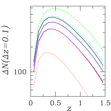
FIG. 8.: The surface density for the SPT survey for different values of $T_{*}$. The dotted line is for $T_{*}=1.0$, the long dashed line (partially hidden) for $T_{*}=1.44$ ($-10\%$), the dot-dashed line for $T_{*}=1.76$ ($+10\%$) and the dashed line for $T_{*}=2.0$. The middle solid line is for the fiducial model, the upper solid line for $\Omega_{\rm m}=0.32$ and the lower solid line for $H_{0}=65\,{\rm km}\,{\rm sec}^{-1}\,{\rm Mpc}^{-1}$. Clearly, differences of $\pm 10\%$ are of the same order of magnitude as the constraints on cosmological parameters which we are trying to establish.

In Fig. 8, we show the variation of the redshift distribution of clusters with varying $T_{*}$. We also show the values for the fiducial model and models with $\Omega_{\rm m}=0.32$ and $H_{0}=65\,{\rm km}\,{\rm sec}\,{\rm Mpc}^{-1}$. We see from this that an uncertainty in $T_{*}$ changes the amplitude in the surface density but not the shape and, therefore, we expect that the degeneracy between the equation of state parameters, which mainly defines the shape of the curves (see Fig. 4), is largely unaffected by this uncertainty. However, we expect degeneracies with $\sigma_{8}$ and $\Omega_{\rm m}$.

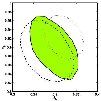
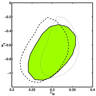
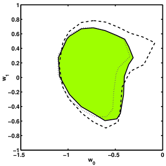
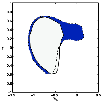
FIG. 9.: The $1-\sigma$ likelihood contours for the SPT survey. In the top two panels and the lower left panel we show the effect of the mass-temperature normalization bias, if we assume $T_{*}$ is $16\%$ larger (dotted) and $12\%$ lower (dashed) than the fiducial value of $T_{*}=1.6$. In the lower right panel $T_{*}$ is included as a free parameter. The inner light shaded contour is with fixed $T_{*}=1.6$ and the outer contour marginalized over $T_{*}$.

In order to test this, we first study the bias we introduce if we analyse mock data, created using a different value of $T_{*}$ than the one we used to perform the analysis. In the top two and lower left panel of Fig. 9 we show the results of this. The dotted line corresponds to a model created with $T_{*}=1.86$ and the dashed line to $T_{*}=1.42$. In all cases we performed the analysis for the fiducial value $T_{*}=1.6$. This roughly corresponds to a bias in the limiting mass of $\pm 20\%$. We see clearly the bias introduced in the $\sigma_{8}$ and $\Omega_{\rm m}$ measurements by choosing the wrong value of $T_{*}$. However, the effect on the dark energy parameters $w_{0}$ and $w_{1}$ (Fig. 9, lower left) seems to introduce only a slight extra bias toward larger $w_{0}$ values and only increases or lowers the errorbars corresponding to the change in the overall number of observed clusters.

This becomes even clearer if we include the parameter $T_{*}$ in the likelihood analysis and marginalize over $T_{*}$. The result of including $T_{*}$ is presented in Fig. 9, lower right panel. We see that this only increases the errorbars in the $w_{0}$ direction. This is because $w_{1}$ (and also partly $w_{0}$) influence mainly the shape of the surface density and not so much its amplitude, as suggested above.

So far we have assumed that the mass-temperature relation applies universally. However, at this stage it is only an observed correlation and is likely to have considerable scatter. Next, we investigate the inclusion of statistical uncertainties in the limiting mass. We incorporate this via a “selection function” $\phi(M,z)$ [25],

$$\frac{dN}{dz}={\Delta\Omega}\frac{dV}{dzd\Omega}(z)\int\limits_{0}^{\infty}\phi(M,z)\frac{dn}{dM}\,dM\,,$$ (31)

with

$$\phi(M,z)=\frac{1}{2}\left\{{\rm erf}\left[\frac{M-M_{\rm lim}(z)}{\delta M_{\rm lim}(z)}\right]+1\right\}\,,$$ (32)

where $\delta$ is the relative statistical uncertainty in the mass limit $M_{\rm lim}$.

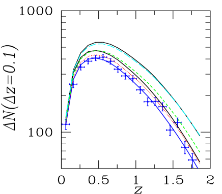
FIG. 10.: The surface density of clusters for the SPT survey. The lowest solid line is for the fiducial model, the middle solid line for $\Omega_{\rm m}=0.32$ and the upper solid line for $\sigma_{8}=0.95$. The dotted line is for a statistical uncertainty in the limiting mass of $\delta=20\%$, the short dashed line for $\delta=30\%$ and the long dashed line for $\delta=40\%$. The data points are from a simulated mock catalogue for the SPT survey.

In Fig. 10 we illustrate the influence of different values of $\delta$ on the observed surface density. A general result is that the inclusion of this effect using a symmetric selection function will always increase the overall number of observed clusters since there are many more objects just below the mass threshold than just above it. We see from the figure that an unknown uncertainty in the limiting mass will also increase the uncertainty in constraints on the cosmological parameters, but if it is known and well understood it should be possible to incorporate it into the analysis. Since the changes in the surface density due to $\delta\neq 0$ only become larger than the expected Poisson errors for SPT when the scatter is greater than $\delta=15\%$, we estimate that a statistical uncertainty below this level should be acceptable for this survey. The Poisson errors for the other surveys are much larger and hence it should be possible for them to withstand much larger values of $\delta$ and still give sensible constraints.

The final uncertainties in the mass temperature relation which we shall investigate are a different power law dependence between $M$ and $T$, and a different overall dependence on redshift [100, 25]. We re-define the mass temperature relation to be

$$\left<T_{\rm e}\right>_{n}=T_{*}\left(\Delta_{c}E(z)^{2}\right)^{1/3}\left[1+\left(1+3w\right)\frac{\Omega_{\rm Q}(z)}{\Delta_{c}}\right]\left(1+z\right)^{\varepsilon-1}\left(\frac{M_{\rm vir}}{10^{15}h^{-1}M_{\odot}}\right)^{1/\xi}\,,$$ (33)

where if $\varepsilon=1$ and $\xi=3/2$ we obtain the standard mass temperature relation (14). Note that new values for $\varepsilon$ and $\xi$ would require a recalibration of the relation and hence a different value of $T_{*}$. However, since we will only restrict ourselves to a qualitative discussion we will not incorporate this effect. The parameter $\xi$ could model non-gravitational heat input. Since smaller clusters (that is, groups) are preferentially affected by these processes, we expect $\xi\geq 1.5$. Observations and simulations suggest values of $1.48\leq\xi\leq 1.98$  [118, 99, 119, 120, 121]. The parameter $\varepsilon$ models deviations from complete virialization. On one hand, clusters at early times might not be completely virialized, hence $\varepsilon<1$. However, clusters which have ongoing mergers or some other form of energy injection could be much hotter than expected and hence have $\varepsilon>1$. At this stage there is no observational preference for any particular value of $\varepsilon$.

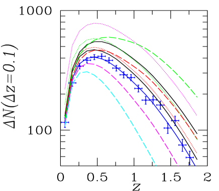
FIG. 11.: The surface density of clusters for the SPT survey with changes in the mass - temperature relation. The lowest solid line is for the fiducial model, the middle solid line for $\Omega_{\rm m}=0.32$ and the upper solid line for $\sigma_{8}=0.95$. The dotted lines are for a change in the power law between limiting mass and temperature. The lowest dotted line is for $\xi=1.6$, the middle dotted line for $\xi=1.7$ and the top for $\xi=1.9$. The long dashed lines are for changes in the redshift dependence of the $M-T$ relation. Form top to bottom the long dashed lines correspond to $\varepsilon=1.5,1.2,0.8,0.5$. The data points are from a simulated mock catalogue for the SPT survey.

In Fig. 11 we illustrate the surface density for the SPT survey for different values of $\xi$ and $\varepsilon$. We allow $\xi$ to vary in the range $\xi=1.6,1.7,1.9$ and see that we observe more clusters for higher values of $\xi$. This is clear since from (10) we obtain $M_{\rm vir}\propto S_{\nu}^{\xi/(\xi+1)}$. This again will increase the uncertainties mainly in the parameters which define the amplitude of the redshift distribution, like $\Omega_{\rm m}$ or $\sigma_{8}$. We vary $\varepsilon$ between $0.5$ and $1.5$. A recent Fisher matrix analysis of SZ cluster counts for the SPT survey obtained uncertainties of $\Delta\xi\approx 0.0064$ and $\Delta\varepsilon\approx 0.46$ [25], if they are included as parameters. Although we believe that a Fisher matrix analysis can only give crude errorbars, we expect degeneracies to not restrict our ability to extract the cosmological parameters. We should note that follow up measurements which constrain the mass of the cluster independently using, for example, X-ray measurements or weak lensing, could constrain the non-standard mass temperature relation considerably [25, 100] and, hence, improve the veracity of constraints on the cosmological parameters deduce from SZ surveys.

B Mass - temperature relation and $\sigma_{8}$

Recent years have seen a wide range of values reported in the literature for the power spectrum normalization $\sigma_{8}$. Observations with weak lensing, X-rays, Large-Scale-Structure and the large scale SZ effect suggest values in the range $0.61\leq\sigma_{8}\leq 1.05$ [122]. If interpreting a particular observations requires the conversion from temperature to mass, as is the case for the SZ effect and X-ray observations, then it is important to know the value of $T_{*}$ which has been used, since there is a direct degeneracy between $\sigma_{8}$ and the normalization $T_{*}$ with $\Omega_{\rm m}^{0.6}\sigma_{8}\propto T_{*}^{-0.8}$ [122]. As noted in the introduction one problem of our analysis is that the choice of a lower value for $\sigma_{8}$ in our fiducial model would have resulted in a lower number of observable clusters and hence much weaker constraints on the cosmological parameters due to the Poisson statistics. However, the analyses of X-ray measurements which result in $0.7\leq\sigma_{8}\leq 0.8$ use a larger value of $T_{*}$ [96, 71, 122]. We will now discuss various aspects of this issue.

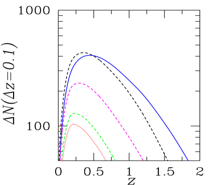
FIG. 12.: The surface density of clusters for the SPT survey. The solid line is for the fiducial parameters and set up. The dotted line is for the same setup, but $\sigma_{8}=0.72$. The dashed lines are for the $\sigma_{8}=0.72$ with $T_{*}$ increasing from $1.8$ (lowest dashed line) via $T_{*}=2.5$ (middle dashed line) to $T_{*}=3.5$ (top dashed line).

In Fig. 12 we illustrate the consequences of combining lower values of $\sigma_{8}$ with larger values of $T_{*}$. The solid line is for the fiducial model and the SPT survey. The dotted line is for the same set up with $\sigma_{8}=0.72$, which seems to be in the preferred range of X-ray and Large-Scale-Structure observations [87, 88, 84]. We see that the overall number of clusters is considerably less for the lower value of $\sigma_{8}$. However, X-ray observations seem to require a lower calibration of the mass temperature relation  [84, 122], which corresponds to an increased value of $T_{*}$. In Fig. 12 we show the increasing number of clusters observed for as $T_{*}$ increases. Still for the marginally maximal acceptable value of $T_{*}=2.5$ [123] the number of clusters is about a factor of $1.7$ below the number observed in a universe with $\sigma_{8}=0.9$. Nonetheless it is clear that the lower values of $\sigma_{8}$ suggested by some lead to the very small number of clusters one would naively assume.

In order to obtain as many clusters predicted in the fiducial model, but using $\sigma_{8}=0.72$ it is necessary to increase to $T_{*}=3.5$, which corresponds to a $75\%$ lower normalization of the mass - temperature relation, outside the range suggested by simulations and measured in reality [123]. Hence, if one is drawn to conclusions of these particular observations it seems likely that our fiducial model over-predicts the number of clusters by at least a factor of two and the errorbars on the parameters we have predict are optimistic. However, there are observations which suggest the opposite. Preliminary observations of secondary CMB anisotropies of the large-scale SZ effect using the CBI instrument [124] indicate a value of $\sigma_{8}>1$ [125]. Although this results remains to be confirmed, it indicates that the issue of the value of $\sigma_{8}$ is far from settled. We should note that it might be possible to measure the normalization of the mass - temperature relation directly with the combination of cluster abundances and weak lensing observations [123] and constrain both $\sigma_{8}$ and $T_{*}$ directly. Furthermore, a measurement of the flux of each cluster will enable one to perform an internal calibration of the sample and alleviate the uncertainty in the normalization of the mass - temperature relation [126].

C Mass function

A further uncertainty we need to consider is the mass function itself. In our analysis we used the 2002 results from the VIRGO consortium [77]. In order to obtain insight into the uncertainty of the mass function we have compared our results to the previously released mass function from 2001 [94]

$$\frac{dn}{dM}\left(z,M\right)=-0.316\frac{\rho_{m}(t_{0})}{M}\frac{d\sigma_{M}}{dM}\frac{1}{\sigma_{M}}\exp\left\{-|0.67-\log\left[D(z)\sigma_{M}\right]|^{3.82}\right\}\,,$$ (34)

with the mass defined by an overdensity of $\Delta=324$ relative to the matter density, which corresponds to an overdensity of $\Delta=97$ relative to the critical density for the fiducial universe. We have also compared our results with the standard PS mass function [92]

$$\frac{dn}{dM}\left(z,M\right)=-\sqrt{\frac{2}{\pi}}\frac{\rho_{m}(t_{0})}{M}\frac{\delta_{c}}{D(z)\sigma_{M}^{2}}\frac{d\sigma_{M}}{dM}\exp\left(-\frac{\delta_{c}^{2}}{2D(z)^{2}\sigma_{M}^{2}}\right)\,$$ (35)

with $\delta_{c}=1.686$, where we ignore the weak cosmology dependence of $\delta_{c}$ in the present discussion.

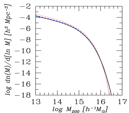
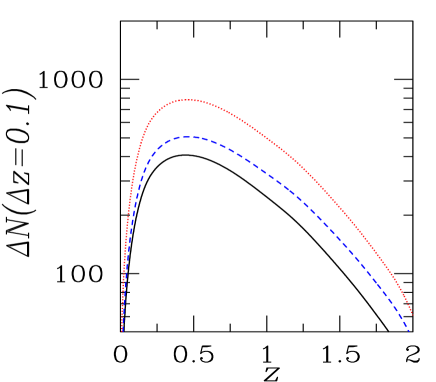
FIG. 13.: On the left the different mass functions at $z=0$. The dashed line is for the Jenkins 2001 mass function [94], the solid line for the Evrard 2002 mass function [77] both from the VIRGO consortium. The dotted line is that expected from the PS formalism for a mass definition of $M_{200}$. On the right the expected surface density of clusters for these mass functions for the SPT survey.

In Fig. 13, we show the different mass function at $z=0$ for the fiducial cosmology. The solid line is for the 2002 mass function of the VIRGO consortium [77], the dashed line for 2001 [94] and the dotted line for the PS mass function. We will investigate the consequences of these three mass functions for expected yield of the SPT survey. Since SPT has a limit of roughly $1.7\times 10^{14}h^{-1}M_{\odot}$ we have to consider the mass function above this limit.The PS function dominates over both the VIRGO 2001 and VIRGO 2002 mass function up to masses of $10^{16}h^{-1}M_{\odot}$ and then PS mass function drops below both VIRGO mass functions. The VIRGO 2001 function is marginally above the VIRGO 2002 function in the range below $10^{16}h^{-1}M_{\odot}$. However, above this region the number of clusters is so sparse that the contribution to the surface density of clusters is not significant. We also present the surface density for the SPT survey in Fig. 13. We see that the PS mass function results in about twice as many clusters and the VIRGO 2001 about $25\%$ more clusters than the VIRGO 2002 mass function. It is clear from this analysis, that a precise convergence of the mass function is required to constrain cosmological parameters using the surface density of clusters, providing further impetus for an extended program of numerical simulations. Clearly the uncertainty in the mass function is degenerate with other uncertainties in the mass - temperature relation and $\sigma_{8}$. However, combining SZ, X-ray and weak lensing of clusters could help constrain the mass function as well.

VI Discussion and conclusions

In this paper we have introduced a realistic model for the surface density of clusters that would be observed by an SZ instrument including effects of the beam of the survey and the profile of the cluster. In the Section IV we analysed constraints on cosmological parameters that might be expected from such surveys. We found that SPT and Planck will be particularly powerful in constraining the standard parameters $\sigma_{8}$ and $\Omega_{m}$, and can be used in conjunction with other observations, for example SNe surveys, to constrain the dark energy. These surveys can be expected on a timescale of around 5 to 7 years. In the meantime less powerful surveys such as those possible using VSA, BOLOCAM, AMI and OCRA will provide useful complementary constraints, while allowing the study of the clusters themselves, in particular using X-ray follow up.

We have shown in Fig. 7 that it is sufficient to use redshift bins of $\Delta z=0.1$ to constrain the cosmological parameters. Essentially the shape of the redshift distribution is mapped out adequately with this bin width. It should be feasible for surveys like SDSS or VISTA [74, 75, 76] to measure redshifts of this accuracy, although one will have to be careful to avoid introducing extra selection effects.

While Planck, SPT and OCRA will constrain the standard cosmological parameters significantly, it will be difficult for them to provide information about the equation of state of the dark energy component. While they do not constrain it by themselves, they are complementary to SNe observations as illustrated in Fig. 7. SZ surveys essentially constrain $\Omega_{m}$ and provide a prior for SNe surveys like the SNAP mission. However, they become considerably more powerful if one includes a tight prior on the amplitude of the density fluctuations $\sigma_{8}$, which could be provided from complementary large scale structure observations.

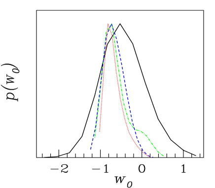
FIG. 14.: The probability for $w_{0}$ marginalized over all the other parameters. The solid line is for the OCRA survey, the short dot-dashed line for SPT, the dashed line for SPT including the parameter $T_{*}$ in the likelihood analysis and the dotted line for SPT with tight priors on $\Omega_{\rm m}$ and $\sigma_{8}$.

This leaves us with the question of whether any of the proposed SZ surveys might be able to distinguish the fiducial cosmology from a $\Lambda$CDM universe. In Fig. 14 we show the one dimensional likelihoods for the constant part of the equation of state $w_{0}$. We see that the OCRA survey can not constrain the equation of state. However the marginalized likelihood of SPT narrows in on the fiducial value of $w_{0}=-0.8$, while with tight priors on $\Omega_{\rm m}$ and $\sigma_{8}$ we can distinguish the fiducial model with $w=-0.8+0.3z$ from a $\Lambda$CDM cosmology.

We have also discussed in detail systematic and statistical uncertainties which might affect more ability to affect our ability to extract cosmological parameters. The main sources of uncertainty are the mass-temperature relation and the mass function; clearly much more work is needed to pin these two quantities down. The inclusion of the normalization factor $T_{*}$ in the likelihood analysis only marginally increases the errorbars on the equation of state state as shown in Fig. 14. A potentially more significant problem is a modified evolution or power law of the mass temperature relation. The Fisher matrix analysis presented in [25] suggests that this problem is not too severe. This is because the cosmological dependence of the surface density is mainly due to the growth factor, rather than that from the limiting mass.

The surveys discussed in this paper will provide much more information than just the surface density. In principle it should be possible to use the flux information as well as the surface density to constrain cosmological parameters as hinted in [100, 126]. However, using the flux as well as redshift information is likely to be more susceptible to systematic error. This subject is currently under investigation.

Finally, we should note that it is difficult to strongly constrain the equation of state of the dark energy component, and particularly its redshift evolution, using any single method. It is clear that a joint effort will be required with a combination of measurements such as those from the cosmic microwave background, large scale structure, SNe, weak lensing and clusters being necessary to achieve this goal. The results presented in this paper show that the SZ effect is likely to play a strong role in this over the next decade.

REFERENCES

- [1] R.A. Sunyaev and Ya. Zel’dovich, Comm. Astrophys. Space Phys. 4, 173 (1972).
- [2] R.A. Sunyaev and Ya. Zel’dovich, MNRAS 190, 143 (1980).
- [3] M. Birkinshaw and A.T. Moffet, Highl. Astron. 7, 321 (1986).
- [4] M. Birkinshaw, in Physical Cosmology (1991), edited by A. Blanchard et al., (Editions Frontieres, Gif sur Yvette, France, 1991).
- [5] J.P. Hughes and M. Birkinshaw, Ap. J. 497, 645 (1998).
- [6] M.E. Jones et al., Nature 365, 320 (1993).
- [7] K. Grainge et al., MNRAS 265, L57 (1993).
- [8] J. Carlstrom, M. Joy, and L.E. Grego, Ap. J. Lett. 456, L75 (1996).
- [9] K. Grainge et al., MNRAS 278, L17 (1996).
- [10] J.E. Carlstrom et al., in Eighteenth Texas Symposium on Relativistic Astrophysics and Cosmology (1998), edited by A. Olinto, J. Frieman, and D. Schramm, (World Scientific, Singapore, 1998).
- [11] E.D. Reese et al., Ap. J. 533, 38 (2000).
- [12] L. Grego et al., Ap. J. 539, 39 (2000).
- [13] S.K. Patel et al., Ap. J. 541, 37 (2000).
- [14] M. Joy et al., Ap. J. Lett. 551, L1 (2001).
- [15] L. Grego et al., Ap. J. 552, 2 (2001).
- [16] P.D. Mauskopf et al., in Imaging at Radio through Submilimeter Wavelength (1999), edited by J. Mangum, (The Astronomical Society of the Pacific, Salt Lake City, 2000).
- [17] J. Glenn et al., in Advanced Technology MMW, Radio, and Terahertz Telescopes (1998), edited by T.G. Phillips, SPIE Proc. Vol. 3357, (SPIE-International Society for Optical Engeneering. Bellingham, WA, 1998).
- [18] R. Kneissl et al., MNRAS 328, 783 (2001).
- [19] M.E. Jones, in AMiBA 2001: High-Z Clusters, Missing Baryons, and CMB Polarization (2001), edited by L. W. Chen, (Astronomical Society of the Pacific, Salt Lake City 2002).
- [20] G.P. Holder et al., Ap. J. 544, 629 (2000).
- [21] J.J. Mohr et al., in Extrasolar Planets in Cosmology: The VLT Opening Symposium (2000), edited by A. Renzini, (Springer, Berlin, 2000).
- [22] J.E. Carlstrom et al., astro-ph/0103480.
- [23] K. Y. Lo et al., in ‘New Cosmological Data and the Values of the Fundamental Parameters’ (2000), edited by A. Lasenby and A. Wilkinson, (Astronomical Society of the Pacific, Salt Lake City, 2002).
- [24] I.W.A. Browne et al., in ’Radio Telescopes’ (2000), edited by H.R. Butcher, SPIE Proc. Vol. 4015, (SPIE-International Society for Optical Engineering, Bellingham, WA, 2000).
- [25] S. Majumdar and J.J. Mohr, Ap. J. 585, 603 (2003).
- [26] J.J. Mohr et al., astro-ph/0208102.
- [27] See at: http://www.hep.upenn.edu/∼angelica/act/act.html
- [28] See at: http://www.mpifr-bonn.mpg.de/div/mm/apex.html
- [29] R.A. Watson et al., astro-ph/0205378.
- [30] B.S. Mason et al., Ap. J. 591, 540 (2003).
- [31] N. Aghanim et al., Astron. Ap. 325, 9 (1997).
- [32] S.T. Kay, A.R. Liddle and P.A. Thomas, MNRAS 325, 835 (2001).
- [33] R.A. Battye and J. Weller, astro-ph/0305465.
- [34] P. Thomas and R.G. Carlberg, MNRAS 240, 1009 (1989).
- [35] J. Oukbir and A. Blanchard, Astron. Ap. 262, L210 (1992).
- [36] R. Scaramella, R. Cen, and J.P. Ostriker, Ap. J. 416, 399 (1993).
- [37] D. Barbosa et al., Astron. Ap. 314, 13 (1996).
- [38] P.T.P. Viana and A.R. Liddle, MNRAS 281, 323 (1996).
- [39] V. Eke, S. Cole and C. Frenk, MNRAS 282, 263 (1996).
- [40] L. Wang and P. J. Steinhardt, Ap. J. 508, 483 (1998).
- [41] E. Pierpaoli, D. Scott and M. White, MNRAS 325, 77 (2001).
- [42] Z. Haiman, J.J. Mohr and G.P. Holder, Ap. J. 553, 545 (2001).
- [43] G. Holder, Z. Haiman, and J.J. Mohr, Ap. J. Lett. 560, L111 (2001).
- [44] A.J. Benson, C. Reichardt, and M. Kamionkowski, MNRAS 331, 71 (2002).
- [45] J. Weller, R.A. Battye, and R. Kneissl, Phys. Rev. Lett. 88, 231301 (2002).
- [46] S. Perlmutter et al., Ap. J. 483, 565 (1997).
- [47] A. Riess et al., Astron. J 116, 1009 (1998).
- [48] S. Perlmutter et al., Ap. J. 517, 565 (1999).
- [49] A. Riess et al., Ap. J. 560, 49 (2001).
- [50] C. Wetterich, Nucl. Phys. B302, 668 (1988).
- [51] P.J.E. Peebles and B. Ratra, Ap. J. 325, L17 (1988).
- [52] B. Ratra and P. J. E. Peebles, Phys. Rev. D37, 3406 (1988).
- [53] C. Wetterich, Astron. Ap. 301, 321 (1995).
- [54] J. Frieman et al., Phys. Rev. Lett. 75, 2077 (1995).
- [55] K. Coble, S. Dodelson and J.A. Frieman, Phys. Rev. D55, 1851 (1997).
- [56] P.G. Ferreira and M. Joyce, Phys. Rev. Lett. 79, 4740 (1997).
- [57] E.J. Copeland, A.R. Liddle and D. Wands, Phys. Rev. D57, 4686 (1998).
- [58] R.R. Caldwell, R. Dave and P.J. Steinhardt, Phys. Rev. Lett. 80, 1582 (1998).
- [59] I. Zlatev, L. Wang and P.J. Steinhardt, Phys. Rev. Lett. 82, 896 (1999).
- [60] P.J. Steinhardt, L. Wang and I. Zlatev, Phys. Rev. D59, 123504 (1999).
- [61] P. Brax and J. Martin, Phys. Lett. B 468, 40 (1999).
- [62] A. Albrecht and C. Skordis, Phys. Rev. Lett. 84, 2076 (2000).
- [63] G. Efstathiou, MNRAS 310, 842 (1999).
- [64] D. Huterer and M.S. Turner, Phys. Rev. D 60, 081301 (1999).
- [65] T.D. Saini et al., Phys. Rev. Lett. 85, 1162 (2000).
- [66] I. Maor, R. Brustein and P.J. Steinhardt [2001], Phys. Rev. Lett. 86, 6. Erratum: Phys. Rev. Lett. 87, 0499901.
- [67] P. Astier, astro-ph/0008306.
- [68] J. Weller and A. Albrecht, Phys. Rev. Lett. 86, 1939 (2001).
- [69] J. Weller and A. Albrecht, Phys. Rev. D65, 103512 (2001).
- [70] V. Sahni et al., JETP Lett. 77, 201 (2003).
- [71] D. Huterer and G. Starkman, Phys. Rev. Lett. 90, 031301 (2003).
- [72] K.-H. Chae et al, Phys. Rev. Lett. 89, 151301 (2002).
- [73] K.-H. Chae, .astro-ph/0211244
- [74] J.E. Gunn and G.R. Knapp, in Sky Surveys: Protostars to Protogalaxies (1993), edited by B.T. Soifer, ASP Conf. Ser. 43, (ASP. San Francisco, CA ,1993).
- [75] J.E. Gunn and D.H. Weinberg, in Wide Field Spectroscopy and the Distant Universe (1995), edited by S.J. Maddox and A. Aragon-Salamanca, (World Scientific. Singapore, 1995).
- [76] S.P. Worsick et al., in Optical Design, Materials, Fabrication, and Maintenance (2000), edited by P. Dierickx, SPIE Proc. Vol. 4003, (SPIE-International Society for Optical Engeneering. Bellingham, WA, 2000).
- [77] A.E. Evrard et al., Ap. J. 573, 7 (2002).
- [78] U. Seljak and M. Zaldarriaga, Ap. J. 469, 437 (1996).
- [79] C. Copi, D.N. Schramm and M.S. Turner, Science 267, 192 (1995).
- [80] S. Burles and D. Tytler, Ap. J. 507, 732 (1998).
- [81] G. Hinshaw et al., astro-ph/0302217.
- [82] U. Seljak, astro-ph/0111362.
- [83] P.T.P. Viana, R.C. Nichol and A.R. Liddle, Ap. J. Lett. 569, L75 (2002).
- [84] S.W. Allen et al., astro-ph/0208394.
- [85] W.L. Freedman et al., Ap. J. 553, 47 (2001).
- [86] R. Bean and A. Melchiorri, Phys. Rev. D65, 041302 (2002).
- [87] A. Lewis and S. Bridle, Phys. Rev. D66, 103511 (2002).
- [88] S.W. Allen, R.W. Schmidt and A.C. Fabian, MNRAS 334, L11 (2002).
- [89] S. L. Bridle, private communication
- [90] P.M. Garnavich et al., Ap. J. 509, 74 (1998).
- [91] S. Perlmutter, M. S. Turner and M. White, Phys. Rev. Lett. 83, 670 (1999).
- [92] W.H. Press and P. Schechter, Ap. J. 187, 452 (1974).
- [93] R.K. Sheth and G. Tormen, MNRAS 323, 1 (2001).
- [94] A. Jenkins et al., MNRAS 321, 372 (2001).
- [95] M. White, Astron. Ap. 367, 27 (2001).
- [96] M. White, Ap. J.Supp. 143, 241 (2002).
- [97] M. Birkinshaw, Phys. Rep. 310, 97 (1999).
- [98] R.A. Battye and J. Weller, In preparation
- [99] J.J. Mohr, B. Mathiesen and A.E. Evrard, Ap. J. 517, 627 (1999).
- [100] L. Verde, Z. Haiman and D. N. Spergel, Ap. J. 581, 5 (2002).
- [101] O. Lahav et al., MNRAS 251, 128 (1991).
- [102] P.B. Lilje, Ap. J. Lett. 386, L33 (1992).
- [103] G.L. Bryan and M.L. Norman, Ap. J. 495, 80 (1998).
- [104] N. Afshordi and R. Cen, Ap. J. 564, 669 (2002).
- [105] R. B. Patridge and P. J. E. Peebles, Ap. J. 147, 868 (1967).
- [106] J. E. Gunn and J. R. Gott, Ap. J. 176, 1 (1972).
- [107] J. F. Navarro, C. S. Frenk and S. D. White, Ap. J. 490, 493 (1997).
- [108] J.G. Bartlett, astro-ph/0001267.
- [109] A. Cavaliere and R. Fusco-Femiano, Astron. Ap. 49, 137 (1976).
- [110] S.M. Molnar and M. Birkinshaw, Ap. J. 537, 542 (2000).
- [111] J.E. Carlstrom, private communication.
- [112] W. Cash, Ap. J. 228, 939 (1979).
- [113] N. Christensen and R. Meyer, astro-ph/0006401.
- [114] N. Christensen et al., Class. Quant. Grav. 18, 2677 (2001).
- [115] N. Sugiyama, Ap. J. S. 100, 281 (1995).
- [116] P.T.P. Viana and A.R. Liddle, MNRAS 303, 535 (1999).
- [117] J. Aldering et al., in Future Research Direction and Visions for Astronomy (2002), edited by A.M. Dressler, SPIE Proc. Vol. 4835, (SPIE-International Society for Optical Engeneering. Bellingham, WA, 2002).
- [118] J.J. Mohr and A.E. Evrard, Ap. J. 517, 627 (1997).
- [119] O. Muanwong et al., astro-ph/0102048.
- [120] H. Xu, G. Jin and X. Wu, astro-ph/0101564.
- [121] A. Finoguenov, T.H. Reiprich and H. Böringer, Astron. Ap. 369, 749 (2001).
- [122] E. Pierpaoli et al., MNRAS 342, 163 (2003).
- [123] D. Huterer and M. White, Ap. J. Lett. 95, 578 (2002).
- [124] J.R. Bond et al., astro-ph/0205386.
- [125] E. Komatsu and U. Seljak, astro-ph/0205468.
- [126] W. Hu, Phys. Rev. D 67, 081304 (2003).