Constraining amplitude and slope of the mass fluctuation spectrum
using cluster baryon mass function.

Abstract

We derive the baryon mass function for a complete sample of low-redshift clusters and argue that it is an excellent proxy for the total mass function if the ratio $f_{b}=M_{b}/M_{\rm tot}$ in all clusters is close to its universal value, $\Omega_{b}/\Omega_{M}$. Under this assumption, the baryon mass function can be used to constrain the amplitude and slope of the density fluctuations power spectrum on cluster scales. This method does not use observational determinations of the total mass and thus bypasses major uncertainties in the traditional analyses based on the X-ray temperature function. However, it is sensitive to possible systematic variations of the baryon fraction as a function of cluster mass. Adapting a weak dependence $f_{b}(M)$ suggested by observations and numerical simulations by Bialek et al., we derive $\sigma_{8}=0.72\pm 0.04$ and the shape parameter $\Omega_{M}h=0.13\pm 0.07$, in good agreement with a number of independent methods. We discuss the sensitivity of these values to other cosmological parameters and to different assumptions about variations in $f_{b}$.

1. Introduction

The number density of galaxy clusters, as a function of mass, is an excellent indicator for the normalization and slope of the power spectrum of the density fluctuations in the present-day Universe. The power spectrum normalization is traditionally expressed in terms of $\sigma_{8}$, the rms amplitude of the density fluctuations on the $8\,h^{-1}$ Mpc scale. In the CDM cosmology, the shape of the present-day power spectrum is controlled almost completely by the product $\Omega_{M}h$ (Bond & Efstathiou 1984). Therefore, the cluster mass function is a sensitive probe of these cosmological parameters.

Considerable progress in the theoretical models of structure formation in the past decade has provided a reliable machinery to compute the shape of the power spectrum for any given set of cosmological parameters (Seljak & Zaldarriaga 1996, Eisenstein & Hu 1998), and to predict the mass function of collapsed objects (clusters) given the power spectrum (Jenkins et al. 2001). Most of the problems with using the cluster mass function as a cosmological probe are on the observational side.

Theory operates with the virial masses of clusters. However, the total cluster mass within the virial radius, as opposed to the mass within a small metric radius, is notoriously difficult to measure. The main techniques such as weak lensing, the X-ray method assuming hydrostatic equilibrium of the intracluster gas, and velocity dispersion of cluster galaxies, lead to significant statistical and systematic uncertainties at large radii, and often produce contradictory results (see e.g., Markevitch & Vikhlinin 1997 and Fischer & Tyson 1997 for representative uncertainty estimates for the X-ray hydrostatic and weak lensing methods, respectively). It is probably fair to say that total masses at the virial radius cannot be determined to better than 30–40% accuracy at present.

Because of the difficulties with the virial mass measurement, a direct derivation of the mass function for a large, complete sample of clusters is not feasible at present. Therefore, the cluster mass is usually related to a more easily measured quantity. Consider one of the most frequently used proxies for the mass function, the cluster temperature function. This relies on the theoretically expected tight correlation $M\propto T^{3/2}$. The theoretically expected slope of the $M-T$ correlation is reproduced both in numerical simulations (Evrard, Metzler & Navarro 1996) and observationally, within a given approach to the total mass measurement (Horner, Mushotzky, & Scharf 1999; Nevalainen, Markevitch & Forman 2000; Finoguenov, Reiprich & Böhringer 2001). However, the normalizations of the $M-T$ relation derived by different authors span a wide range (see Evrard et al. 2002 for a review). Ultimately, the question of the normalization of the $M-T$ relation boils down to the possibility of total mass measurements with small systematic uncertainties, which is at the limits of current observational techniques.

The expected cluster mass functions are very steep and therefore any change in the mass scale leads to large variations of the derived cosmological parameters. In a recent review, Rosati et al. (2002) estimated that 30% uncertainties in the normalization of the $M-T$ relation leads to a 20% uncertainties in $\sigma_{8}$ and 30% uncertainties in $\Omega_{M}$ derived from cluster evolution. Until the $M-T$ relation is reliably normalized, precise measurements of the cosmological power spectrum from the cluster temperature function are impossible. Therefore, it is desirable to explore new proxies for the cluster mass function that would not require absolute measurements of the total mass. In this Paper, we propose that such a proxy can be based on the easily measured cluster baryon masses.

Indeed, it is expected that the fraction of baryons in the virial mass of clusters equals the average value in the Universe — $f_{b}\equiv M_{b}/M_{\text{tot}}=\Omega_{b}/\Omega_{M}$ (White et al. 1993). Therefore, the baryon fraction is the same for clusters of any mass at any redshift at least to a first approximation. This is one of the best-proved cluster-related facts, that is justified by basic theory, confirmed by numerical simulations (e.g., Frenk et al. 1998), and supported observationally (Mohr, Mathiesen & Evrard 1999, Allen et al. 2002). Given the universality of the baryon fraction, there is a trivial relation between the cumulative total and baryon mass functions:

$$F_{b}(M_{b})=F_{\text{tot}}(\Omega_{M}/\Omega_{b}M_{b}).$$ (1)

The average baryon density in this equation is fixed by either the Big Bang Nucleosynthesis theory or by the cosmic microwave background fluctuations, $\Omega_{b}h^{2}=0.0224\pm 0.0009$ (Spergel et al. 2003). The baryon mass is a convenient proxy for the total mass because 1) it is easily derived from the X-ray imaging observations (§ 3), and 2) the scaling between $M_{b}$ and $M_{\text{tot}}$ is expressed in terms of the model parameters ($\Omega_{M}$) and therefore does not rely on the absolute total mass measurements. In this Paper, we apply this method to ROSAT observations of a complete flux-limited sample of 52 low-redshift clusters selected from the All-Sky Survey data.

The Paper is organized as follows. In § 2, we describe selection of our cluster sample. The measurements of the baryon masses are presented in § 3 and the baryon mass function is derived in § 4. The theory involved in modeling the baryon mass function is reviewed in § 5. In § 6, we derive constraints on $\sigma_{8}$ and on the shape parameter, $\Gamma=\Omega_{M}h$, and discuss the dependence of these results on our basic assumption of the universality of the baryon fraction.

Numerical values of the cluster parameters are quoted for the $H_{0}=71$ km s^-1 Mpc^-1, $\Omega_{M}=0.3$ and $\Lambda=0.7$ cosmology.

2. Cluster Sample

Table 1Cluster sample

Object	$z$	$T$${}^{\text{\it a}}$	$f_{x}$${}^{\text{\it b}}$	$L_{x}$	$M_{g,324}$	$M_{b,324}$	$r_{g,324}$	$L_{\text{opt}}$${}^{\text{\it c}}$
		(keV)		$10^{44}$ erg s-1	$10^{14}M_{\odot}$	$10^{14}M_{\odot}$	(Mpc)	$10^{13}L_{\odot}$
2A0335	0.0349	3.6	6.8	1.8	$0.59\pm 0.07$	$0.78\pm 0.10$	1.85	$\cdots$
A85	0.0556	6.9	4.3	3.0	$1.11\pm 0.13$	$1.35\pm 0.16$	2.24	$0.41\pm 0.06$
A119	0.0442	5.6	2.4	1.0	$1.00\pm 0.10$	$1.27\pm 0.13$	2.19	$\cdots$
A262	0.0155	2.2	4.6	0.2	$0.20\pm 0.04$	$0.31\pm 0.06$	1.31	$0.09\pm 0.03$
A399	0.0715	6.8	1.7	2.0	$1.21\pm 0.31$	$1.62\pm 0.38$	2.27	$\cdots$
A400	0.0238	2.3	1.6	0.2	$0.25\pm 0.02$	$0.38\pm 0.04$	1.41	$0.11\pm 0.03$
A401	0.0739	8.0	3.1	3.9	$2.34\pm 0.26$	$2.82\pm 0.31$	2.82	$0.47\pm 0.18$
A478	0.0882	6.9	4.5	8.2	$2.16\pm 0.24$	$2.59\pm 0.29$	2.71	$0.36\pm 0.09$
A496	0.0328	4.7	5.4	1.3	$0.61\pm 0.08$	$0.80\pm 0.11$	1.87	$\cdots$
A576	0.0389	4.0	1.6	0.5	$\cdots$	$0.46\pm 0.14$${}^{\text{*}}$	$\cdots$	$\cdots$
A754	0.0542	9.8	4.3	2.9	$1.58\pm 0.16$	$1.90\pm 0.20$	2.52	$\cdots$
A1060	0.0137	3.2	6.1	0.2	$0.20\pm 0.04$	$0.29\pm 0.06$	1.31	$\cdots$
A1367	0.0214	3.7	4.7	0.5	$0.41\pm 0.07$	$0.54\pm 0.09$	1.66	$0.14\pm 0.04$
A1644	0.0474	4.7	2.2	1.1	$0.92\pm 0.21$	$1.19\pm 0.25$	2.11	$\cdots$
A1651	0.0860	6.2	1.5	2.6	$1.14\pm 0.17$	$1.42\pm 0.21$	2.19	$\cdots$
A1656	0.0231	8.1	18.2	2.1	$1.54\pm 0.18$	$1.91\pm 0.23$	2.57	$0.51\pm 0.11$
A1736	0.0461	3.6	1.7	0.8	$\cdots$	$0.66\pm 0.20$${}^{\text{*}}$	$\cdots$	$\cdots$
A1795	0.0622	6.0	3.9	3.4	$0.93\pm 0.08$	$1.15\pm 0.11$	2.10	$0.25\pm 0.04$
A2029	0.0766	9.1	4.3	5.7	$1.86\pm 0.24$	$2.30\pm 0.29$	2.60	$0.58\pm 0.12$
A2052	0.0353	3.4	3.0	0.8	$0.31\pm 0.05$	$0.42\pm 0.07$	1.49	$0.13\pm 0.03$
A2063	0.0355	3.7	2.5	0.7	$0.44\pm 0.07$	$0.60\pm 0.09$	1.68	$0.17\pm 0.03$
A2065	0.0726	5.4	1.4	1.7	$\cdots$	$1.13\pm 0.34$${}^{\text{*}}$	$\cdots$	$\cdots$
A2142	0.0894	9.3	3.9	7.3	$3.13\pm 0.23$	$3.73\pm 0.28$	3.06	$0.56\pm 0.09$
A2147	0.0353	4.4	3.1	0.9	$1.01\pm 0.18$	$1.33\pm 0.22$	2.21	$\cdots$
A2163	0.2010	11.5	1.4	14.6	$5.58\pm 0.74$	$6.41\pm 0.85$	3.37	$\cdots$
A2199	0.0299	4.8	6.5	1.3	$0.57\pm 0.04$	$0.75\pm 0.06$	1.84	$0.24\pm 0.04$
A2204	0.1523	7.1	1.6	9.4	$2.07\pm 0.43$	$2.51\pm 0.49$	2.52	$\cdots$
A2256	0.0581	7.3	3.7	2.8	$1.48\pm 0.12$	$1.80\pm 0.15$	2.45	$0.54\pm 0.06$
A2589	0.0416	3.7	1.6	0.6	$0.29\pm 0.04$	$0.42\pm 0.06$	1.46	$\cdots$
A2634	0.0309	3.3	1.5	0.3	$0.31\pm 0.04$	$0.42\pm 0.05$	1.50	$0.19\pm 0.03$
A2657	0.0400	3.7	1.7	0.6	$0.40\pm 0.05$	$0.54\pm 0.06$	1.62	$\cdots$
A3112	0.0750	5.3	1.9	2.5	$0.81\pm 0.13$	$1.03\pm 0.16$	1.98	$\cdots$
A3158	0.0591	5.8	2.3	1.8	$0.90\pm 0.15$	$1.17\pm 0.19$	2.09	$\cdots$
A3266	0.0589	8.0	3.5	2.8	$1.71\pm 0.17$	$2.05\pm 0.20$	2.57	$\cdots$
A3376	0.0455	4.0	1.4	0.6	$0.41\pm 0.06$	$0.54\pm 0.07$	1.63	$\cdots$
A3391	0.0514	5.7	1.5	0.9	$0.93\pm 0.14$	$1.24\pm 0.18$	2.12	$\cdots$
A3395	0.0506	5.0	1.9	1.1	$1.24\pm 0.20$	$1.59\pm 0.25$	2.33	$\cdots$
A3526	0.0112	3.4	15.7	0.4	$0.31\pm 0.05$	$0.44\pm 0.07$	1.51	$\cdots$
A3558	0.0480	5.5	4.0	2.1	$1.34\pm 0.12$	$1.66\pm 0.16$	2.39	$\cdots$
A3562	0.0490	5.2	1.8	1.0	$0.92\pm 0.09$	$1.17\pm 0.13$	2.12	$\cdots$
A3571	0.0391	7.2	7.5	2.5	$1.21\pm 0.18$	$1.50\pm 0.22$	2.33	$\cdots$
A3581	0.0214	1.8	2.0	0.2	$\cdots$	$0.23\pm 0.07$${}^{\text{*}}$	$\cdots$	$\cdots$
A3667	0.0556	7.0	4.6	3.2	$2.50\pm 0.24$	$2.99\pm 0.29$	2.93	$\cdots$
A4038	0.0292	3.3	3.6	0.7	$0.31\pm 0.05$	$0.44\pm 0.07$	1.50	$\cdots$
A4059	0.0460	4.4	2.0	0.9	$0.45\pm 0.07$	$0.62\pm 0.09$	1.67	$\cdots$
EXO 0422	0.0390	2.9	1.9	0.6	$\cdots$	$0.53\pm 0.16$${}^{\text{*}}$	$\cdots$	$\cdots$
Hydra A	0.0522	3.6	2.9	1.8	$0.60\pm 0.07$	$0.77\pm 0.09$	1.83	$\cdots$
MKW 3s	0.0453	3.7	2.1	1.0	$0.40\pm 0.06$	$0.53\pm 0.08$	1.60	$\cdots$
MKW 4	0.0210	1.7	1.4	0.1	$0.14\pm 0.01$	$0.21\pm 0.03$	1.15	$0.05\pm 0.02$
NGC1550	0.0120	1.1	2.5	0.1	$0.05\pm 0.01$	$0.08\pm 0.02$	0.84	$\cdots$
NGC507	0.0155	1.3	1.5	0.1	$0.08\pm 0.01$	$0.13\pm 0.02$	0.97	$\cdots$
S 1101	0.0580	2.6	1.5	1.1	$0.29\pm 0.04$	$0.39\pm 0.06$	1.43	$\cdots$

^a Cluster temperatures adapted from Markevitch et al. (1998, 1999), White et al. (2000), Fukazawa et al. (1998), David et al. (1993), Arnaud et al. (2001), Blanton et al. (2001), Horner et al. (1999), Allen & Fabian (1998), Finoguenov et al. (2001), Kaastra et al. (2001), Sun et al. (2003)

^b X-ray flux in 0.5–2.0 keV, in $10^{-11}$erg s^-1 cm^-2 units.

^c Optical luminosity inside $r_{g,324}$ in the V band, adapted from Arnaud et al. (1992), Hradecky et al. (2000), Beers et al. (1984).

^∗ — baryon mass determined from $M_{b,324}-L_{x}$ correlation.

Our cluster sample was selected from the HIFLUGCS catalog (Reiprich & Böhringer 2002) of clusters selected from the ROSAT All-Sky Survey (RASS) data. This catalog includes 63 clusters above a flux limit of $2\times 10^{-11}$ erg s^-1 cm^-2 in the 0.1–2.4 keV band, detected over 2/3 of the sky.

We have applied further objective selections to facilitate a more reliable measurement of the baryon mass function. First, we increased the flux limit to $1.4\times 10^{-11}$ erg s^-1 cm^-2 in the 0.5–2 keV band (or $2.3\times 10^{-11}$erg s^-1 cm^-2 in the 0.1–2.4 keV band). Second, we considered only clusters at $z>0.01$ because at lower redshifts, the virial radius of most objects does not fit inside the ROSAT field of view. In total, 52 clusters from the HIFLUGCS catalog satisfied our selection criteria (Table 1).

Most of the selected objects were observed by ROSAT in one or more pointed observations, so high-quality X-ray data are available. Several more clusters are so bright that their baryon mass can be measured from the shallower RASS data. For only 5 clusters, A576, A1736, A2065, A3581, and EXO422, the existing X-ray data do not permit a direct baryon mass measurement at the virial radius, so we used the $M_{b}-L_{x}$ correlation to estimate their masses.

3. Baryon mass measurement

3.1. ROSAT Data Reduction and Gas Mass Measurements

The data were prepared in a standard manner. For pointed observations, we used S. Snowden’s software (Snowden et al. 1994) to produce flat-fielded images with all non-sky background components removed. For the RASS data, we used the archive-supplied exposure maps. Experiments with different energy bands show that the 0.7–2 keV band has the optimal ratio of cluster to background surface brightness. Our further analysis is performed in this band.

The measurement of the gas mass profile from the X-ray imaging data was performed almost identically to the approach described in Vikhlinin, Forman & Jones (1999). We first extracted the azimuthally-averaged surface brightness profile centered on the apparent centroid of the cluster. The background level was estimated by fitting the profile at large radii, $0.3r_{v}<r<1.5r_{v}$ where $r_{v}$ is the virial radius estimated from the X-ray temperature, with the power law plus constant model. The power law here represents the cluster brightness and the constant corresponds to the background. The background intensity was subtracted from the profile assuming that it is constant across the image,

Assuming that the clusters are spherically symmetric, the gas density profiles were derived from the surface brightness profiles using direct deprojection (Fabian et. al. 1981). The deprojection method yields the radial profile of the X-ray volume emissivity which is easily converted to the gas density as $n_{e}=K\,\varepsilon^{1/2}$, $\rho_{g}=1.15n_{e}m_{p}$, where the numerical value for $K$ can be found for any plasma temperature using the MEKAL code (Mewe et al. 1985), and the numerical value in the second relation corresponds to the standard mix of fully ionized hydrogen and helium.

For three clusters, A1060, A1644, and NGC1550, the ROSAT surface brightness profile were too noisy for direct deprojection. We resorted to the usual $\beta$-model analysis in these three cases.

The intracluster gas which we directly observe in X-rays is the dominant baryonic component of clusters. We will use the cluster masses corresponding to the density contrast $\delta=324$ relative to the mean density of the Universe at the redshift of observation (see § 5 below). Therefore, we derive the gas masses from the following equation: $3M_{g}(<\!r)/(4\pi r^{3}\,\langle\rho_{b}\rangle)=324$, where $M_{g}(<\!r)$ is the gas mass profile as derived from the X-ray data. We adopt the average baryon density as given by the WMAP observations of the cosmic microwave background fluctuations, $\langle\rho_{b}\rangle=6.23\,(1+z)^{3}$ $M_{\odot}$ kpc^-3 (or $\Omega_{b}\,h^{2}=0.0224$, Spergel et al. 2003) which is also close to the Big Bang Nucleosynthesis value of $\Omega_{b}\,h^{2}=0.020$ (Burles, Nollett & Turner 2001). The observed X-ray surface brightness profiles permit a direct measurement of the gas mass at the radius corresponding to $\delta=324$.

The measured gas masses $M_{g,324}$ are listed in Table 1. It is useful to provide simple relations which allow one to scale our results to other values of the mean overdensity, Hubble constant etc. Empirically, we find that on average, the radial dependence of mass is $M(\theta)\propto\theta$, which corresponds to the following scaling as a function of overdensity

$$M_{\delta}\propto\delta^{-0.5}.$$ (2)

Within a fixed aperture, the X-ray derived baryon mass scales as $h^{-5/2}$. There is an additional scaling because $M_{\delta}$ is measured at a fixed overdensity $\delta$ rather than within a fixed angular radius. The angular radius corresponding to the overdensity $\delta$ is found from the equation $M(\theta_{\delta})/(\theta_{\delta}^{3}h^{-3})=\mathrm{const}$. Given the empirical average mass profile, $M(\theta)\propto\theta$, and the $h$-scaling of $M(\theta)$, $\theta_{\delta}$ should scale as $h^{0.25}$, and therefore

$$M_{\delta}\propto h^{-2.25}.$$ (3)

The only effect of changing the average baryon density in the Universe is to change the apparent mean overdensity, and so one can use eq. (2) to convert our masses to $\delta=324$ for a different value of $\Omega_{b}\,h^{2}$:

$$M_{\delta}\propto(\Omega_{b}h^{2})^{-0.5}.$$ (4)

Figure 1.— Correlation of the optical luminosity of the cluster in the V band and the gas mass ($M_{g,324}$). The original optical measurements were extrapolated to $r_{g,324}$ as explained in the text. The solid line shows the best-fit power law (eq. 5)

3.2. Stellar Mass in Clusters

The stellar material in galaxies contributes a small but non-negligible fraction of the cluster baryon mass. Not all clusters in our sample have high-quality optical observations. Therefore, we first use the published data for a subsample of our clusters to establish a correlation of the optical luminosity with the gas mass and then use this correlation to estimate the stellar contribution in all clusters.

The optical luminosities for 16 clusters were compiled from the papers by Arnaud et al. (1992), Hradecky et al. (2000), and Beers et al. (1984). The optical luminosities in these papers are quoted at different metric radii in the V band, and so we converted them to the gas overdensity radius $r_{324}$ assuming that the light follows the King profile with $r_{c}=180$ kpc (Bahcall 1975). The resulting luminosities within $r_{324}$ show a very tight correlation with the gas mass (Fig. 1) which is fitted by the following relation

$$L_{\text{opt}}=319L_{\odot}\,\bigg{[}\frac{M_{g,324}}{M_{\odot}}\bigg{]}^{0.71}$$ (5)

We further assume the same mass-to-light ratio for the stars, $M_{*}/L_{\text{opt}}=6M_{\odot}/L_{\odot}$ in the V band, which follows from the stellar evolution models for the average population of elliptical and spiral galaxies in clusters (Arnaud et. al. 1992). Under these assumptions, equation [5] can be used to estimate the total baryon (i.e. gas plus galactic stars) mass of a cluster from the X-ray measured gas mass:

$$\frac{M_{b,324}}{M_{g,324}}=1.100+0.045\,\biggl{[}\frac{M_{g,324}}{10^{15}M_{\odot}}\biggl{]}^{-0.5}.$$ (6)

Therefore, galactic stars contribute about 15% of the total baryon mass in massive clusters, and this fraction slightly increases in the less massive systems. This estimate of the stellar contribution is consistent with the considerations presented in Fukugita, Hogan & Peebles (1998). The trend in the stellar-to-gas ratio is similar to that derived by Lin, Mohr & Stanford (2003) using the $K$-band photometry from the 2MASS survey, although the overall normalization of $M_{*}/M_{g}$ is smaller in that paper.

We ignore any contribution from intergalactic stars to the cluster baryon mass. At present this component cannot be reliably estimated. However, all available studies (e.g., Feldmeier et al. 2002) suggest that the intergalactic stars contribute only a small fraction to the total stellar mass of the cluster, and therefore only a few percent at most to the total baryon mass.

3.3. Baryon Mass Error Budget

The main contribution to the mass measurement uncertainty is the Poisson noise in the X-ray surface brightness profiles. This noise component is straightforward to compute in each case. Typically, the statistical uncertainty in the baryon mass is about 20%. All other uncertainties are systematic and we can only estimate their contribution.

We measured the baryon masses under the assumption that the clusters are spherical. Any deviations from the spherical symmetry result in a scatter in our mass determination. We estimate this scatter to be 7% based on the azimuthal scatter of the gas mass profiles (Vikhlinin et al. 1999) and from the results of numerical simulations by Mathiesen, Evrard & Mohr (1999).

The stellar mass was estimated using a number of assumptions. First, we assumed a standard mass-to-light ratio for the galactic stars. Second, the total light was estimated from the extrapolation of the King profile to large radii. Third, for most clusters, the optical luminosity was estimated from the $L_{\text{opt}}-M_{\text{g}}$ relation which has some scatter (Fig. 1). We conservatively estimate that the stellar mass is measured with a 30% uncertainty. The stellar mass is only 15–20% of the gas mass, therefore the contribution to the uncertainty in the total baryon mass is small (5–7%).

The final uncertainties on the baryon mass were obtained by adding the above three components in quadrature. The dominant contribution is still the statistical noise in the X-ray data.

Figure 2.— Cluster baryon mass as a function of the total X-ray luminosity in the 0.5–2 keV band. The solid line shows the best fit power law and dashed lines indicate the 1$\sigma$ scatter around the mean relation.

3.4. Correlation of the X-ray Luminosity and the Baryon Mass

The key relation for estimating the mass functions is the volume of the survey as a function of mass. For a flux-limited sample like ours, the volume is determined by the scaling relation between the mass and the X-ray luminosity. Such a relation is also useful for estimating the masses in those cases where direct mass measurements are impossible.

Our sample was selected using the total (i.e. without excluding either substructures or cooling flow regions) X-ray fluxes in the 0.5–2 keV band. Therefore, the $M_{b}-L_{x}$ correlation should be with the total luminosity in this energy band. The corresponding measurements are listed in Table 1 and plotted in Fig. 2. The average $M_{b,324}-L_{x}$ correlation is well fitted by the power law

$$M_{b,324}=8.5\times 10^{13}M_{\odot}\times(L_{x}/10^{44}\,\mathrm{erg~{}s^{-1}})^{0.78\pm 0.04}$$ (7)

where the best-fit parameters were found using the bisector method of Akritas & Bershady (1996) and the uncertainty in the slope was estimated using bootstrap resampling.

There is a significant scatter in the $M_{b,324}-L_{x}$ correlation which can be partly explained by the contribution of cooling flow regions and substructures to the total cluster flux. As Figure 3 shows, the scatter around the mean relation is well approximated by the log-normal distribution with an rms scatter of $\sigma_{\lg M}=0.19$ in mass. Part of this scatter is due to the mass measurement errors. Subtracting this contribution in quadrature, we find that the intrinsic log scatter in the $M_{b,324}-L_{x}$ correlation is $\sigma_{\lg M}=0.17$ in mass for a given luminosity or $\sigma_{\lg L}=0.15$ in luminosity for a given mass.

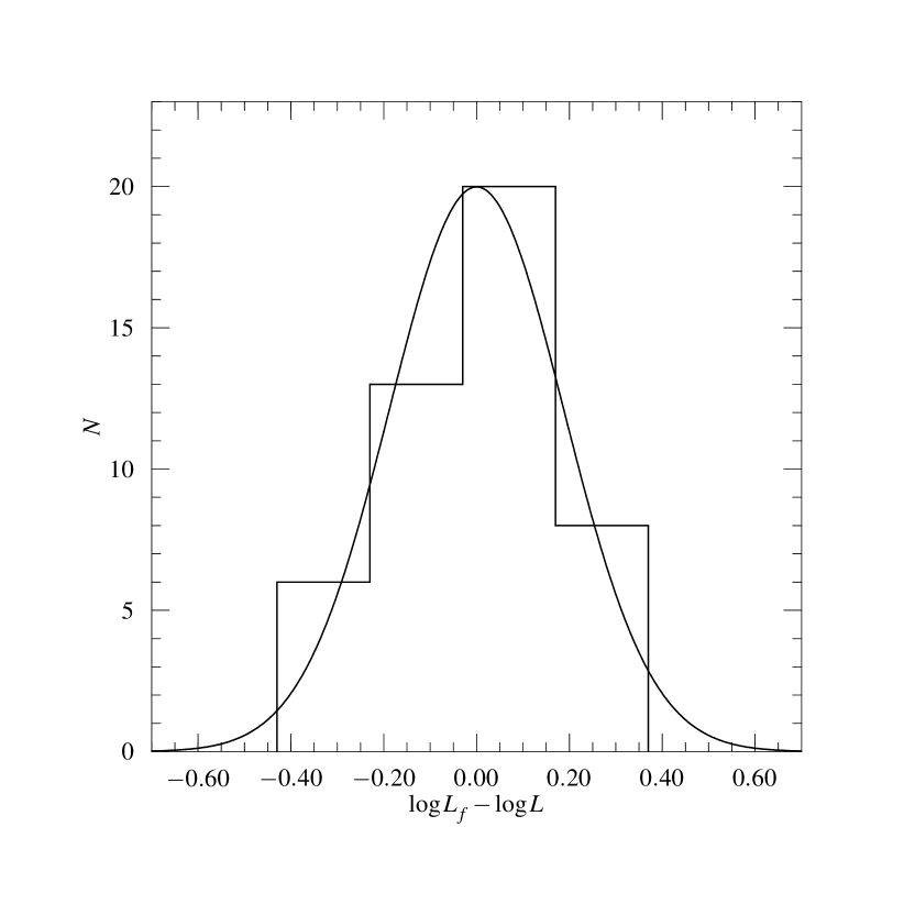
Figure 3.— Deviations of the measured luminosity from the mean $M_{b}-L_{x}$ relation. Solid line shows the Gaussian fit.

4. Observed Baryon Mass Function

The volume of a flux-limited survey for the cluster of luminosity $L$ is obtained by integration of the cosmological dependence of comoving volume, $dV/dz$, over the redshift interval $z_{\text{min}}-z_{\text{max}}$, where $z_{\text{min}}$ is the lower redshift cut (0.01 in our case), and $z_{\text{max}}$ is the maximum redshift for the cluster to exceed the flux limit, $f_{\text{lim}}$:

$$f_{\text{lim}}(0.5-2)=\frac{L\left(0.5(1+z_{\text{max}})-2(1+z_{\text{max}})\right)}{4\pi\,d_{L}^{2}(z_{\text{max}})},$$ (8)

where $d_{L}(z_{\text{max}})$ is the luminosity distance as a function of redshift. The solution of this equation with respect to $z_{\text{max}}$ leads to the survey volume as a function of cluster luminosity, $V(L)$.

Given the probability distribution $p(L|M)$ of the cluster luminosity for the given mass, the survey volume as a function of mass is computed as $V(M)=\int p(L|M)V(L)\,dL$. Taking into account the average relation between $M_{b}$ and $L$ (eq. 7) and the log-normal scatter around this relation, we obtain:

$$\begin{split}V(M)=&\frac{1}{(2\pi)^{1/2}\sigma_{\lg M}}\;\times\\ &\int\exp\biggl{[}-\frac{(\lg L_{f}(M)-\lg L)^{2}}{2\sigma_{\lg M}^{2}}\biggl{]}V(L)\,d\lg L,\end{split}$$ (9)

where $L_{f}(M)$ is given by the inverse of eq. (7). The sample volume as a function of the cluster baryon mass is shown in Fig. 4.

Figure 4.— Sample volume as a function of the cluster baryon mass.

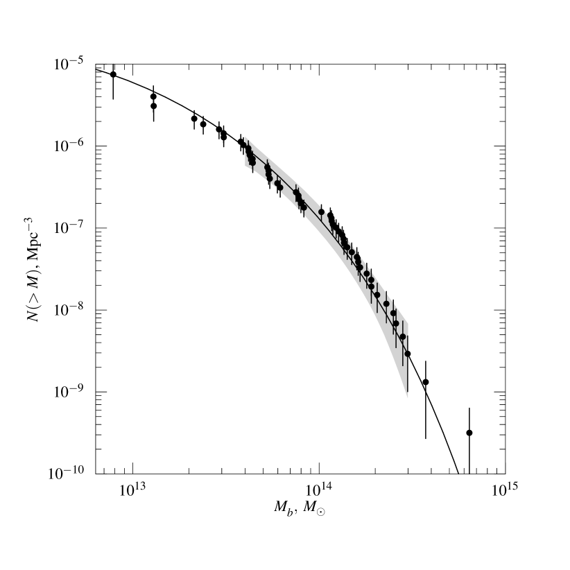
Figure 5.— Local baryon mass function. The gray band shows a 68% uncertainty interval derived from the Maximum Likelihood analysis including the mass measurement errors. The solid line corresponds to the prediction of our best-fit cosmological model (Fig. 6).

We will use the cumulative representation of the mass function which is estimated from observations as

$$f(M)=N(>M)=\sum_{M_{i}\geq M}\frac{1}{V(M_{i})},$$ (10)

where $V(M_{i})$ is given by eq. [9]. The resulting baryon mass function is shown in Fig. 5.

There are two contributions to the uncertainty in the $f(M)$ measurement — the Poisson noise which is trivially estimated as

$$\left(\Delta_{P}f(M)\right)^{2}=\sum_{M_{i}\geq M}\frac{1}{V^{2}(M_{i})},$$ (11)

and the component related to the mass measurement uncertainties. To take both components into account, we performed the Maximum-Likelihood fits of the measured $f(M)$ with a two-parameter Schechter function $df/dM=A(M/M_{0})^{\alpha}\exp(-M/M_{0})$ (Schechter 1976). The likelihood function was constructed to include the scatter due to the mass measurement errors (for details, see Voevodkin, Vikhlinin & Pavlinsky 2002 and Vikhlinin et al. 2003). The range of statistically acceptable parameters $A$, $\alpha$, and $M_{0}$ defines a band of the cumulative mass functions consistent with the data at the given confidence level. The resulting 68% uncertainties in the $f(M)$ measurement are shown as a grey band in Fig. 5. For reasons explained below (§ 6), we use only clusters with baryon mass $M_{b}>4\times 10^{13}M_{\odot}$ for the theoretical modeling. Therefore, the Schechter function fits were performed only in this mass range.

In addition to the statistical uncertainty in the mass function there is an additional component because of the cosmic variance in a survey of a finite volume. Hu & Kravtsov (2003) calibrate the ratio of the cosmic variance and Poisson noise as a function of cluster mass. Using their results, we find that the cosmic variance is negligible in our mass range for $\sigma_{8}\simeq 0.7-0.8$ indicated by our data (see below).

5. Review of Theory

Recent numerical simulations of structure formation in the Universe provide accurate analytic expressions for the cluster total mass function (Jenkins et al. 2001). Jenkins et al. have demonstrated that the mass functions in the CDM cosmology has a universal form when expressed as a function of the linear rms density fluctuations on the mass scale $M$, $\sigma(M)$:

$$\frac{M}{\langle\rho\rangle}\frac{dN(>\!M)}{d\log\sigma(M)}=A\exp\,(-|\log\sigma^{-1}+b\,|^{c})$$ (12)

All dependencies of the mass function on cosmological parameters enter through $\sigma(M)$. The function $\sigma(M)$ is equivalent to the power spectrum of linear density perturbations (Peebles 1981). We will assume that the power spectrum, $P(k)$, is the product of the primordial inflationary spectrum $k^{n}$ and the CDM transfer function: $P(k)\sim k^{n}T^{2}(k)$. The transfer function depends on the parameters $\Omega_{M}$, $h$, and $\Omega_{b}$. We used analytic approximations to $T(k)$ provided by Eisenstein & Hu (1998). Therefore, the theoretical model for the mass function is defined by parameters $\Omega_{M}$, $\Omega_{b}$, $h$, $n$, and also the normalization of the power spectrum, $\sigma_{8}$.

The numerical values of coefficients $A$, $b$, and $c$ in (12) depend on the definition of the cluster mass. The most convenient definition, from the observational point of view, is the mass corresponding to a given spherical overdensity, $\delta$, relative to the mean density at the cluster redshift. Jenkins et al. considered two values of $\delta$, 180 and 324 (the latter value corresponds to the virial radii in the $\Lambda$CDM model with $\Omega_{M}=0.3$). We measured baryon masses for $\delta=324$. For this overdensity, Jenkins et al. obtain $A=0.316$, $b=0.67$, and $c=3.82$.

If the baryon fraction in clusters is indeed universal, the baryon and total overdensities must be equal, $\delta=\delta_{b}$, which allows one to use the measured baryon mass $M_{b,324}$ as a proxy for the total mass, $M_{324}$. Recall that the model for the baryon and total mass function are related via equation (1).

Using the machinery described above, we can compute the model for the baryon mass function for any set of cosmological parameters and then fit it to the observations, self-consistently rescaling the observed mass function to the cosmological parameters being tried. In the rest of this section, we consider separately the effect of each cosmological parameter on the $F_{b}(M_{b})$ model and on scaling of the observed mass function. We also consider the effect of possible deviations of $M_{b}/M_{\text{tot}}$ from the universal value.

5.1. Parameter $\Omega_{M}$

Parameter $\Omega_{M}$, mainly through the product $\Omega_{M}h$, determines the shape of the transfer function $T(k)$ and therefore the slope of the mass function. This is a strong effect which allows us to derive $\Omega_{M}$ from the cluster mass function.

In addition, $\Omega_{M}$ affects the growth of density perturbations. This effect should be taken into account, because the observational mass function is derived in a redshift interval of finite width. Therefore, we computed the mass function models at several redshifts and weighted them with the survey volume for the given mass.

The effect of $\Omega_{M}$ on the observed mass function via the mass and volume calculations is very weak and can be ignored. The growth factor also depends on $\Lambda$, but very weakly at low redshift, and therefore we fixed $\Lambda=0.7$.

5.2. Power Spectrum Normalization $\sigma_{8}$

The normalization of the mass function model is exponentially sensitive to $\sigma_{8}$, which allows a precise determination of this parameter from the observed cluster abundance.

The baryon mass measurements do not depend on $\sigma_{8}$, so there is no associated scaling of the observed mass function.

5.3. Hubble Constant $h$

The derived baryon masses are very sensitive to the value of $h$, $M_{b,324}\propto h^{-2.25}$ (eq. 3), and so the observed mass function must be scaled accordingly. In the mass function model, the Hubble constant enters through the product $\Omega_{M}h$ (see above) and also changes the mass scale, $M\propto h^{-1}$ (see e.g. Jenkins et al.). The normalization of the model mass function scales as $h^{3}$, and, obviously, the observed mass function scales identically.

Although the Hubble constant measurements now converge to $h=0.71$ (Freedman et al. 2001, Spergel et al. 2003), our method is quite sensitive to $h$. To determine the appropriate scalings, we varied $h$ in the range from 0.5 to 0.8. We use $h=0.71$ for a baseline model.

5.4. Average Baryon Density $\Omega_{b}h^{2}$

The average baryon density in the Universe is known quite accurately, $\Omega_{b}h^{2}=0.0224\pm 0.0009$ (Spergel et al. 2003, see also Burles et al. 2001). This parameter enters the measurement of the baryon masses $M_{b,324}$ (§ 3.1, eq. (4)), the scaling between the models for the total and baryon mass functions (eq. 1), and, weakly, the shape of the transfer function. Variations of $\Omega_{b}h^{2}$ within the above uncertainty range result in negligible changes in either the observed or theoretical mass function. We, however, allowed $\Omega_{b}h^{2}$ to vary in a broader range, from 0.018 to 0.025. If not stated explicitly, all the results below are reported for $\Omega_{b}h^{2}=0.0224$.

5.5. Primordial Power Spectrum Slope $n$

The observed mass function is independent of the power spectrum. For the model mass function, the effect of $n$ is indistinguishable from that of the product $\Omega_{M}h$ because our entire mass range corresponds to a narrow (factor of 2) wavenumber range, where the power spectrum of density perturbations is indistinguishable from a power law. Our parameter constraints below were generally obtained for $n=1$, expected in the inflationary models (Starobinskii 1982, Guth & Pi 1982, Hawking 1982) and favored by the recent CMB observations (Spergel et al. 2003). The $n$-dependence of the derived parameter values was studied by varying $n$ in the range from 0.85 to 1.15.

5.6. Non-Universality of the Baryon Fraction $\Upsilon$

Our method depends on the assumption that the baryon fraction in clusters is universal, $M_{b}/M_{\text{tot}}=\Omega_{b}/\Omega_{M}$. Any large deviations from the universality may have serious observational and methodological implications, and therefore require special attention.

Consider first how the baryon mass measurements have to be scaled, if the baryon fraction is non-universal. Let us assume that at large radii, baryons still follow the dark matter, i.e. $M_{b}/M_{\text{tot}}=\Upsilon\,\Omega_{b}/\Omega_{M}$ where $\Upsilon$ is a constant for each cluster. The first obvious correction is to multiply the baryon mass by $\Upsilon^{-1}$. However, if $\Upsilon\neq 1$, the baryon and total overdensities at each radius are different, $\delta_{b}=\Upsilon\delta$. We need the baryon mass which corresponds to the total overdensity $\delta=324$, and therefore the baryon mass measurements must be corrected by an additional factor of $\Upsilon^{-0.5}$ (cf. eq. 2). Overall, the baryon mass measurement must be scaled by a factor of $\Upsilon^{-1.5}$.

Consider now the effect of possible variants for the non-universality of the cluster baryon fraction. Most of the deviations of $\Upsilon$ from unity can be factorized into the following three possibilities:

1) $\Upsilon\neq 1$, but is the same for all clusters. Such a deviation accounts for any systematic under- or overabundance of baryons in clusters. Such a deviation is often observed in numerical experiments (Mathiesen et al. 1999 and references therein). Any systematic bias in the X-ray based gas mass measurement is also indistinguishable from $\Upsilon\neq 1$. For example, Mathiesen et al. show that a systematic 5–10% overestimation of the gas mass is possible because of deviations from spherical symmetry. Overall, 15% variations of $\Upsilon$ seem to include the range for all known effects. We studied the dependence of our results on such a systematic change of $\Upsilon$ by repeating all the analyses for $\Upsilon=0.85$, 1.0, and 1.15.

2) $\Upsilon=1$ on average, but there is some cluster-to-cluster scatter. This can be represented by a convolution of the baryon mass function model with the appropriate kernel. We find, that the effect on the derived parameters is negligible as long as the scatter of $\Upsilon$ remains small ($\lesssim 15\%$), which is supported observationally (Mohr et al. 1999).

3) $\Upsilon$ is a function of the cluster mass and $\Upsilon\rightarrow 1$ in massive clusters. This type of variation of the baryon fraction is expected, e.g., in the models which involve a significant preheating of the intergalactic medium. As a toy model for $\Upsilon(M)$, we considered the parameterization

$$\Upsilon(M_{b})=1-\frac{M_{*}}{M_{b}},\,\,M_{*}=0.7\times 10^{13}M_{\odot},$$ (13)

which describes the results of numerical simulations by Bialek et al. (2001) where the level of preheating was adjusted so that the simulated clusters reproduce the observed $L_{x}-T$ relation. This relation also is reasonably consistent with recent direct measurements of the baryon fraction in a small number of clusters spanning a temperature range of 1.5–10 keV (Pratt & Arnaud 2002, 2003; Sun et al. 2003, Allen et al. 2002).

Equation [13] was used as our baseline model in deriving the parameter constraints, but we also considered all of the above possibilities for deviations of $\Upsilon$ from unity.

The results of this section can be briefly summarized as follows. Given a set of parameters $\Omega_{M}$, $h$, $\sigma_{8}$, $n$, $\Omega_{b}$, we compute the linear power spectrum of density perturbations (Eisenstein & Hu 1998), then convert it to the model for the total mass function (Jenkins et al. 2001) and apply to the observed baryon mass function scaled along the mass axis as follows (here, $\omega_{b}=\Omega_{b}h^{2}$)

$$Mh^{-1}=\Upsilon^{-1.5}M_{b}\frac{\Omega_{M}h^{2}}{\omega_{b}}\biggl{(}\frac{h}{0.71}\biggl{)}^{-2.25}\biggl{(}\frac{\omega_{b}}{0.0224}\biggl{)}^{-0.5}$$ (14)

6. Results

6.1. Application of the Models to the Data

In the previous section, we discussed how to compute a model for the baryon mass function for a given set of CDM model parameters. Parameter constraints can be obtained by fitting such models to the observed mass function using the Maximum Likelihood (ML) method. Note, however, that an exact computation of the likelihood in our case is rather cumbersome because of the presence of the mass measurement uncertainties in addition to the Poisson noise (§ 4). To avoid the computational overhead, we used a simpler technique to derive the cosmological parameter constraints. We use 68% and 95% confidence bands for the mass function obtained in § 4 using an ML fit to the Schechter function. A mass function model which is entirely within a 68% confidence band in the interesting mass range is deemed acceptable at the 68% confidence level (and likewise for the 95% confidence level). Further comparison of this and ML methods is given in Vikhlinin et al. (2003).

This method results in slightly more conservative confidence intervals than a direct ML fitting. An advantage of our approach over ML fits is its direct relation to the goodness-of-fit information. By design, all acceptable mass function models actually fit the data. On the contrary, the goodness-of-fit information is generally unavailable with the ML approach and sometimes it is possible to obtain artificially narrow confidence intervals on parameters only because the best fit model provides a poor fit to the data.

For parameter constraints, we considered the observed baryon mass function in a restricted mass range, $4\times 10^{13}M_{\odot}\leq M_{b}\leq 3\times 10^{14}M_{\odot}$. The choice of the lower limit is motivated by the possibility that the baryon fraction drops systematically in the less massive clusters (see above). Also, the number of clusters in our sample with $M_{b}<4\times 10^{13}M_{\odot}$ is small and so the effects of incompleteness may be important. The upper limit of the mass interval was chosen to exclude the two most massive and potentially peculiar clusters A2142 and A2163 (Fig. 5).

Figure 6.— Confidence intervals (68% and 95%) for the baseline model ($h=0.71$, $n=1$, $\Omega_{b}h^{2}=0.0224$, and $\Upsilon$ from eq. [13]).

As was discussed in § 5, the most sensitive constraints from the cluster baryon mass function are for parameters $\sigma_{8}$ and $\Omega_{M}h$. Other parameters, $h$, $n$, $\Omega_{b}h^{2}$, cannot be constrained from such an analysis. Their variation causes simple scalings of the constraints on $\sigma_{8}$ and $\Omega_{M}h$. Below, we will describe constraints on $\sigma_{8}$ and $\Omega_{M}h$ for the baseline model, $h=0.71$, $n=1$, $\Omega_{b}h^{2}=0.0224$, and provide scalings of these constraints corresponding to variations of the latter three parameters as well as deviations of $\Upsilon(M)$ from the adopted model. We consider separately the $\sigma_{8}-\Omega_{M}h$ constraints from fitting the shape of the mass function in the $4\times 10^{13}M_{\odot}\leq M_{b}\leq 3\times 10^{14}M_{\odot}$ mass range and from using only the normalization of the mass function at $M_{b}=1.0\times 10^{14}\,M_{\odot}$.

6.2. Fitting the Shape of the Baryon Mass Function

A simultaneous determination of the parameters $\sigma_{8}$ and $\Omega_{M}h$ is possible from fitting the mass function in a broad $M$-range because the slope of the mass function is sensitive to $\Omega_{M}h$ and its normalization — to $\sigma_{8}$. In Fig. 6, we show the 68% and 95% confidence regions for our baseline model. The best fit is obtained for $\Omega_{M}h=0.13$ and $\sigma_{8}=0.72$ (the corresponding mass function model is shown by the solid line in Fig. 5). The 68% uncertainty interval on $\Omega_{M}h$ includes the ‘Cosmic Concordance’ value of $\Omega_{M}=0.3$, but the confidence regions are skewed towards lower values of $\Omega_{M}$. This result is similar to a conclusion from the cluster temperature function studies that the cluster mass function is shallower than predicted in CDM (Henry 2000).

Parameter $h$: Consider now how the $\sigma_{8}-\Omega_{M}h$ constraints depend on the exact value of $h$. The effect of the Hubble constant on the shape of the power spectrum is important only through the product $\Omega_{M}h$. Therefore, the effect of $h$ is to shift the confidence levels in Fig. 6 along the $\sigma_{8}$ axis. Experimenting with different values of $h$, we find that this shift is

$$\Delta\sigma_{8}=0.31\Delta h.$$ (15)

Note that the $\sigma_{8}$ constraints derived from the cluster temperature function are independent of $h$ because both the mass corresponding to a given $T$ and the independent variable of the model mass function scale as $h^{-1}$. In our case, a different scaling of the baryon mass measurement with $h$ ($M_{b}\propto h^{-2.25}$, see § 5) leads to a dependence of the derived $\sigma_{8}$ on $h$.

Parameter $n$: The shape of the cluster mass function is defined by the slope of the linear power spectrum of density perturbations in the narrow wavenumber range around $k\sim 0.1h$, where $P(k)$ is accurately approximated by a power law. This means that we cannot disentangle the slope of the primordial (inflationary) power spectrum $n$ from the slope of the transfer function on cluster scales. For example, for a higher value of $n$ we need a flatter transfer function, i.e., a lower value of $\Omega_{M}h$. Therefore, our $\sigma_{8}-\Omega_{M}h$ constraints computed for $n=1$ (Fig. 6) simply move along the $\Omega_{M}h$ axis when the assumed value of $n$ is changed:

$$\Delta(\Omega_{M}h)=-0.21\Delta n.$$ (16)

Figure 7.— The effect of variations in the baryon fraction on the cosmological constraints. The solid contour corresponds to $\Upsilon$ given by eq. [13] (baseline model), the dotted contour is obtained for the case of a $10\%$ cluster-to-cluster scatter in $\Upsilon$ around the mean relation [13], and the dashed contour corresponds to $\Upsilon=1$.

Parameter $\Omega_{b}h^{2}$: This parameter affects the mass function model via the transfer function, but the effect is miniscule for reasonable values of $\Omega_{b}/\Omega_{M}$. The effect of the average baryon density on the observed baryon mass function (via the scaling of $M_{b}$, eq. 4) is much stronger. This effect is equivalent to the $h$-scaling of $M_{b}$ considered above — it shifts the $\sigma_{8}-\Omega_{M}h$ confidence intervals along the $\sigma_{8}$ axis,

$$\Delta\sigma_{8}=-18.0\,\Delta\Omega_{b}h^{2}$$ (17)

Non-universal baryon fraction, $\Upsilon$: As we noted before, any large deviations of the cluster baryon fraction from the universal value $\Omega_{b}/\Omega_{M}$ can significantly affect our results.

The simplest case is a uniform scaling of the baryon fraction by a factor $\Upsilon_{0}$, i.e. $\Upsilon(M)=\Upsilon_{0}(1-M_{*}/M_{b})$ for our baseline model (eq. 13) or simply $\Upsilon(M)=\Upsilon_{0}$. Such a variation in $\Upsilon$ simply shifts the observed baryon mass fraction along the mass axis by a factor of $\Upsilon_{0}^{1.5}$ (eq. 14). The effect on the $\sigma_{8}-\Omega_{M}h$ confidence intervals is the same as in the case of variations of $\Omega_{b}h^{2}$ and $h$ — the confidence intervals shift along the $\sigma_{8}$ axis,

$$\Delta\sigma_{8}=-0.37\Delta\Upsilon_{0},$$ (18)

and the constraints on $\Omega_{M}h$ are unaffected.

If $\Upsilon$ is a function of the cluster mass, as in (13), the shapes of the total and baryon mass functions are different (cf. eq. 14). Therefore, the derived values of both $\sigma_{8}$ and $\Omega_{M}h$ are affected. The results of fitting the observed mass function assuming either $\Upsilon(M)$ given by equation (13) or $\Upsilon(M)=1$ are shown in Fig. 7. For $\Upsilon(M)=1$, we obtain lower values of both $\Omega_{M}h$ and $\sigma_{8}$ (dashed contour), although the effect on $\sigma_{8}$ is partly due to the correlation of this parameter with the assumed value of $\Omega_{M}$ (see below). If the baryon fraction decreases in low-mass clusters, the cumulative baryon mass function is progressively shifted towards smaller $M$. This makes the predicted $F(M_{b})$ flatter with a smaller normalization than for $\Upsilon=1$. Therefore, the data will require steeper models for the total mass functions (i.e., higher values of $\Omega_{M}h$) with a higher normalization (i.e., higher values of $\sigma_{8}$).

Dotted contour in Fig. 7 shows the effect of a 10% cluster-to-cluster scatter in $\Upsilon$ on the $\sigma_{8}-\Omega_{M}h$ constraints. As expected, the scatter has a small effect on the results, only to expand the size of the confidence interval by $\sim 12\%$.

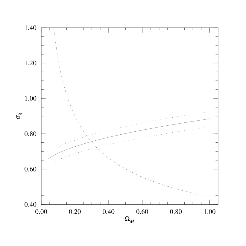
Figure 8.— Constraints on $\sigma_{8}$ using only the normalization of the baryon mass fraction and assuming $h=0.71$. The dotted lines correspond to the 68% confidence region and the solid line shows the analytic approximation (eq. [19]). The dashed line shows a typical $\sigma_{8}(\Omega_{M})$ dependence obtained from the normalization of the cluster temperature function (adapted from Seljak 2002).

6.3. Constraints from Normalization of the Baryon Mass Function

The $\sigma_{8}$ constraints are often derived from the cluster abundance data by using only the normalization of the mass or temperature functions, e.g., the number density of $T>6$ keV clusters. We have applied this approach to our baryon mass function data. The number density of clusters with $M_{b}>10^{14}M_{\odot}$, the median mass in the sample, was used as the only observable. This mass threshold approximately corresponds to clusters with $T=5.5$ keV (from the $M_{b,324}-T$ relation presented in Voevodkin et al. 2002). Since no information about the shape of the mass function is used, it is possible to constrain only $\sigma_{8}$ as a function of $\Omega_{M}$. The results are shown in Fig. 8 by dotted lines. The allowed band (68% confidence) of $\sigma_{8}$ for our baseline model is accurately described by the following equation (solid line in Fig. 8):

$$\sigma_{8}(\Omega_{M})=0.60+0.28\,\Omega_{M}^{0.5}\pm 0.04.$$ (19)

The $\sigma_{8}$ constraints from the normalization of the cluster temperature or total mass functions are also $\Omega_{M}$-dependent. Typically, one finds $\sigma_{8}\propto\Omega_{M}^{-\alpha}$ with $\alpha=0.4-0.6$ from these analyses. Our $\Omega_{M}$-dependence is much weaker (solid vs. dashed line in Fig. 8). The dependence of $\sigma_{8}$ on $\Omega_{M}$ in the baryon mass function analysis is weak, because the relation between the cluster baryon mass and the corresponding linear scale is $\Omega_{M}$-independent, $\lambda^{3}\sim M_{b}/\langle\rho_{b}\rangle$, while for the total mass, $\lambda^{3}\sim M_{\text{tot}}/(\Omega_{M}\,\rho_{\text{cr}})$. This is one of the advantages of our method. The price we have to pay is the introduction of new dependencies for the derived value of $\sigma_{8}$ on parameters $h$, $\Omega_{b}\,h^{2}$, and $\Upsilon$. Table 2 summarizes the changes in the coefficients of equation (19) as these parameters are varied.

Table 2Variations of $a$ and $b$ in the relation $\sigma_{8}(\Omega_{M})=a+b\Omega_{M}^{0.5}$ as the main parameters are changed.

Parameter	$\Delta a$	$\Delta b$
$h$	$0.15$	$0.47$
$\Omega_{b}h^{2}$	$-6.17$	$-23.7$
$\Upsilon$ from eq. (13)	$-0.08$	$-0.63$
$\Upsilon=\mathrm{const}$	$-0.12$	$-0.51$

7. Comparison with earlier work

Determination of $\sigma_{8}$ from various datasets at $z=0$ is a well-established field and so a comparison of our results with at least some recent relevant studies is in order.

Our results can be most directly compared with the determination of $\sigma_{8}$ from the cluster abundance data. Most such studies use the cluster temperature as a proxy for the total mass and a normalization of the local temperature function at $T=5-7$ keV as the primary observable. A review of recent results from the temperature function can be found in Pierpaoli et al. (2003). As we noted before, the scatter in the derived values of $\sigma_{8}$ in this method is mostly due to different assumptions regarding the normalization of the $M-T$ relation. Generally, our determination of $\sigma_{8}$ is in excellent agreement (for $\Omega=0.3$) with those studies that use the $M-T$ normalization from the X-ray total mass measurements assuming hydrostatic equilibrium for the ICM (e.g., Markevitch 1998, Seljak 2002). Our $\sigma_{8}$ is lower than the determination from the optical cluster mass function by Girardi et al. (1998). However, our value (for $\Omega_{M}=0.3$) is consistent with the analyses of Bahcall et al. (2003) who used the cluster mass function estimated from the Sloan Digital Sky Survey, and of Melchiorri et al. (2003) who combined the SDSS results with the pre-WMAP CMB measurements.

Two papers have used essentially the local X-ray luminosity function (XLF) and the X-ray normalized $L_{x}-M_{\text{tot}}$ relation (Reiprich & Böhringer 2002, Allen et al. 2003) to estimate the total mass function. Our results on $\sigma_{8}$ are in a good agreement with these works (for $\Omega=0.3$). Reiprich & Böhringer also fit the shape of their mass function to derive $\Omega_{M}h=0.09\pm 0.03$. This is consistent but on the low side of our confidence intervals (Fig. 6), likely because Reiprich & Böhringer used the Press-Schechter approximation for the mass function in their modeling which is less accurate than the Jenkins et al. fit employed here.

Matter density fluctuations can be traced by the spatial distribution of galaxies. Two modern surveys, SDSS and 2dF (York et al. 2000, Colless et al. 2001) provide excellent datasets for these studies. The galaxy power spectrum from 2dF implies $\Omega_{M}h=0.20\pm 0.03$ (Percival et al. 2001), consistent with our results for the baseline model.

Using clusters as tracers of large scale structure is also a promising approach to determine the matter power spectrum. Using the power spectrum of 426 clusters from the REFLEX survey (Böhringer et al. 2001), Schuecker et al. (2003) determine $\sigma_{8}=0.71\pm 0.03$ and $\Omega_{M}h=0.24\pm 0.02$. Note that this method is probably less sensitive to the normalization of the $M_{\rm tot}-L_{x}$ relation than using the normalization of the XTF or XLF because the bias factor changes more slowly than the spatial density of clusters as a function of mass (Mo & White 1996). It is encouraging that our results are in good agreement with the Schuecker et al. values.

Finally, $\sigma_{8}$ can be determined from the fluctuations of the cosmic microwave background. The recent WMAP measurements of the CMB angular fluctuations and Thompson optical depth of the Universe indicate $\sigma_{8}=0.9\pm 0.1$ assuming pure CDM, $w=-1$, and some other common cosmological priors (Spergel et al. 2003); this is higher than, but consistent with, our value.

8. Summary and Conclusions

We have derived the baryon mass function for galaxy clusters at a median redshift $\langle z\rangle=0.05$. The baryon (gas+stars) mass is measured within a radius of mean baryon overdensity $\delta=324$, using direct deprojection of the ROSAT X-ray imaging data (for gas mass) and an established correlation between $M_{\rm g}$ and $L_{\rm opt}$ (for stellar mass).

We argue that if the baryon fraction in cluster is nearly universal, the baryon mass function is an excellent proxy for the total mass function — $F(M_{\rm tot})$ is obtained from $F_{b}(M_{b})$ simply by a constant log shift along the mass axis. In fact, $F_{b}(M_{b})$ contains enough information to derive the amplitude and slope of the density fluctuations at cluster scales, even if the absolute value of $M_{\rm tot}/M_{b}$ is unknown.

Using this method we obtain $\sigma_{8}=0.72\pm 0.04$ and $\Omega_{M}h=0.13\pm 0.07$. The baryon mass function method has an important advantage in that it does not rely on rather uncertain observational determinations of the total cluster mass. The tradeoff is the sensitivity of the derived values of $\sigma_{8}$ and $\Omega_{M}h$ to other cosmological parameters (such as $h$, $\Omega_{b}$). Our method is also sensitive to any significant deviations of the cluster baryon fraction from universality (§ 6). However, the good agreement of our results with a large number of measurements by other, independent methods (§ 7) shows that our assumptions about the weak trends in the baryon fraction are reasonable. We hope that future progress in observations and physical models of the ICM will reduce this uncertainty to such a level that easily measurable baryon masses can be used as a reliable proxy for the total mass at all redshifts.

References

- (1)
- (2) Akritas, M., & Bershady, M. 1996, ApJ, 470, 706
- (3)
- (4) Allen, S. & Fabian, A. 1998, MNRAS, 297, L57
- (5)
- (6) Allen, S. W., Schmidt, R. W., & Fabian, A. C. 2002, MNRAS, 334, L11
- (7)
- (8) Arnaud, M., Neumann, D., Aghanim, N., Gastaud, R., Majerowicz, S., & Hurhes, J. 2001, A&A, 365, 80
- (9)
- (10) Arnaud, M., Rothenflug, R., Boulade, O., Vigroux, L. & Vangion-Flam, E. 1992, 254, 49
- (11)
- (12) Bahcall, N, 1975, ApJ, 198,249
- (13)
- (14) Bahcall, N. A. et al. 2003, ApJ, 585, 182
- (15)
- (16) Beers, T., Geller, M., Huchra, J., Latham, D. & Davis, R. 1984, ApJ, 283, 33
- (17)
- (18) Bialek, J. J., Evrard, A. E., & Mohr, J. J. 2001, ApJ, 555, 597
- (19)
- (20) Blanton, E., Sarazin, C., McNamara, B., & Wise, M. 2001, 558, 15
- (21)
- (22) Böhringer, H. et al. 2001, A&A, 369, 826
- (23)
- (24) Bond, J. R. & Efstathiou, G. 1984, ApJ, 285, L45
- (25)
- (26) Burles, S., Nollett, K. M., & Turner, M. S. 2001, ApJ, 552, L1
- (27)
- (28) Colless, M. et al. 2001, MNRAS, 328, 1039
- (29)
- (30) David, L., Slyz, A., Jones, C., Forman, W., Vrtilek., S. D. & Arnaud, K. A. 1993, ApJ, 412, 479
- (31)
- (32) Eisenstein, D. J., & Hu, W. 1998, ApJ, 496, 605
- (33)
- (34) Evrard, A. E., Metzler, C. A., & Navarro, J. F. 1996, ApJ, 469, 494
- (35)
- (36) Evrard, A. E. et al. 2002, ApJ, 573, 7
- (37)
- (38) Fabian, A., Hu, E., Cowie, L. & Grindlay, J. 1981, ApJ, 248, 47
- (39)
- (40) Feldmeier, J. J., Mihos, J. C., Morrison, H. L., Rodney, S. A., & Harding, P. 2002, ApJ, 575, 779
- (41)
- (42) Finoguenov, A., Reiprich, T. & Böhringer, H. 2001, A&A, 368, 749
- (43)
- (44) Fischer, P. & Tyson, J. 1997, ApJ, 114, 14
- (45)
- (46) Freedman, W. L. et al. 2001, ApJ, 553, 47
- (47)
- (48) Fukazawa, Y. et al. 1998, PASJ, 50, 187
- (49)
- (50) Fukugita, M., Hogan, C. J. & Peebles, P. J. E. 1998, ApJ, 503, 518
- (51)
- (52) Girardi, M., Borgani, S., Giuricin, G., Mardirossian, F., & Mezzetti, M. 1998, ApJ, 506, 45
- (53)
- (54) Guth, A. H. & Pi, S.-Y. 1982, Physical Review Letters, 49, 1110
- (55)
- (56) Hawking,, S. W. 1982, Phys. Letters, 115B, 295
- (57)
- (58) Henry, J. P. 2000, ApJ, 534, 565
- (59)
- (60) Horner, D. J., Mushotzky, R. F. & Scharf, C. S. 1999, ApJ, 520, 78
- (61)
- (62) Hradecky, V., Jones, C., Donnelly, R., Djorgovski, S., Gal, R. & Odewahn, S. 2000, ApJ, 553, 521
- (63)
- (64) Hu, W. & Kravtsov, A. V., 2003, ApJ, 584, 702
- (65)
- (66) Kaastra, J., Ferrigo, C., Tamura, T., Paerels, F., Peterson, J., Mittaz, J. 2001, A&A, 365,99
- (67)
- (68) Jenkins, A., Frenk, C. S., White, S. D. M., Colberg, J. M., Cole, S., Evrard, A. E., Couchman, H. M. P., & Yoshida, N. 2001, MNRAS, 321, 372
- (69)
- (70) Lin, Y., Mohr, J. J., & Stanford, S. A. 2003, ApJ, 591, 749
- (71)
- (72) Markevitch, M. 1998, ApJ, 504, 27
- (73)
- (74) Markevitch, M. & Vikhlinin, A. 1997, ApJ, 491, 467
- (75)
- (76) Markevitch, M., Forman, W., Jones, C., Sarazin, C., & Vikhlinin, A. 1998, ApJ, 503, 77
- (77)
- (78) Markevitch, M., Vikhlinin, A., Forman, W., Sarazin, C., & Vikhlinin, A. 1999, ApJ, 527, 545
- (79)
- (80) Mathiesen, B., Evrard, A. E. & Mohr, J.J 1999, ApJ, 520, L21
- (81)
- (82) Melchiorri, A., Bode, P., Bahcall, N. A., & Silk, J. 2003, ApJ, 586, L1
- (83)
- (84) Mo, H. J. & White, S. D. M. 1996, MNRAS, 282, 347
- (85)
- (86) Mohr, J. J., Mathiesen, B., & Evrard, A. E. 1999, ApJ, 517, 627
- (87)
- (88) Mewe, R., Gronenschild, E. H. B. M. & van den Oord, G. H. J. 1985, A&AS, 62, 197
- (89)
- (90) Nevalainen, J., Markevich, M. & Forman, W. 2000, ApJ, 532, 694
- (91)
- (92) Percival, W. J. et al. 2001, MNRAS, 327, 1297
- (93)
- (94) Peebles, P. J. E. 1980, The Large-Scale Structure of the Universe (Princeton Univ. Press)
- (95)
- (96) Pierpaoli, E., Borgani, S., Scott, D., & White, M. 2003, MNRAS, 342, 163
- (97)
- (98) Ponman, T., Cannon, D. & Navarro, J. 1999, Nature, 397, 135
- (99)
- (100) Pratt, G. W. & Arnaud, M. 2002, A&A, 394, 375
- (101) Pratt, G. W. & Arnaud, M. 2003, A&A, 408, 1
- (102)
- (103) Reiprich, T. N., Böhringer, H. 2002, ApJ, 567, 716
- (104)
- (105) Seljak, U. 2002, MNRAS, 337, 769
- (106)
- (107) Seljak, U. & Zaldarriaga, M. 1996, ApJ, 469, 437
- (108)
- (109) Snowden, C., McCammon, D., Burrows, D. & Mendenhall, J. 1994, ApJ, 424, 714
- (110)
- (111) Spergel, D. N. et al. 2003, ApJS, 148, 175
- (112)
- (113) Starobinskii, A. A. 1982, Phys. Lett., 117B, 175
- (114)
- (115) Sun, M., et al. 2003, ApJ, in press (astro-ph/0308037)
- (116)
- (117) Vikhlinin, A., Forman, W. & Jones, C. 1999, ApJ, 525, 47
- (118)
- (119) Vikhlinin, A., VanSpeybroeck, L., Markevitch, M., Forman, W. R., & Grego, L. 2002, ApJ, 578, L107
- (120)
- (121) Vikhlinin, A., et al. 2003, ApJ, 590, 15
- (122)
- (123) Voevodkin, A., Vikhlinin, A. & Pavlinsky, M. 2002, Astron. Letters, 28, 793
- (124)
- (125) White, S. D. M., Navarro, J. F., Evrard, A. E., & Frenk, C. S. 1993, Nature, 366, 429
- (126)
- (127) White, D. 2000, MNRAS, 312, 663
- (128)
- (129) York, D. G. et al. 2000, AJ, 120, 1579
- (130)