¹¹institutetext: Astronomical Institute of St.Petersburg State University, Universitetskii pr. 28, Petrodvoretz, 198504 Russia

The structure and evolution of M 51-type galaxies

Abstract

We discuss the integrated kinematic parameters of 20 M 51-type binary galaxies. A comparison of the orbital masses of the galaxies with the sum of the individual masses suggests that moderately massive dark halos surround bright spiral galaxies. The relative velocities of the galaxies in binary systems were found to decrease with increasing relative luminosity of the satellite. We obtained evidence that the Tully–Fisher relation for binary members could be flatter than that for local field galaxies. An enhanced star formation rate in the binary members may be responsible for this effect. In most binary systems, the direction of orbital motion of the satellite coincides with the direction of rotation of the main galaxy. Seven candidates for distant M 51-type objects were found in the Northern and Southern Hubble Deep Fields. A comparison of this number with the statistics of nearby galaxies provides evidence for the rapid evolution of the space density of M 51-type galaxies with redshift $z$ . We assume that M 51-type binary systems could be formed through the capture of a satellite by a massive spiral galaxy. It is also possible that the main galaxy and its satellite in some of the systems have a common cosmological origin.

keywords:

galaxies, groups and clusters of galaxies

1 Introduction

M 51-type (NGC 5194/95) binary systems consist of a spiral galaxy and a satellite located near the end of the spiral arm of the main component. Previously (Klimanov and Reshetnikov 2001), we analyzed the optical images of about 150 objects that were classified by Vorontsov-Vel’yaminov (1962–1968) as galaxies of this type. Based on this analysis, we made a sample of 32 objects that are most likely to be M 51-type galaxies. By analyzing the sample galaxies, we were able to formulate empirical criteria for classifying a binary system as an object of this type (Klimanov and Reshetnikov 2001):

(1) the $B$ -band luminosity ratio of the components ranges from 1/30 to 1/3;

(2) the satellite lies at a projected distance that does not exceed two optical diameters of the main component.

Klimanov et al. (2002) presented the results of spectroscopic observations of 12 galaxies from our list of M 51-type objects, including rotation curves for the main galaxies and line-of-sight velocities for their satellites. Together with previously published results of other authors, we have access to kinematic data for most (20 objects) of our selected M 51-type galaxies. Here, we analyze the observational data for the galaxies of our sample. All of the distance-dependent quantities were determined by using the Hubble constant H₀ = 75 km s^-1 Mpc^-1 (except Section 4).

2 Mean parameters of the galaxy sample

Refer to caption — Figure 1: Left: The distribution of observed line-of-sight velocity differences between the main galaxy and its satellite. Right: The velocity difference between the main galaxy and its satellite versus the projected linear separation between them.

The kinematic parameters for 12 binary systems were published by Klimanov et al. (2002) (see Fig. 1 and the table in this paper). The corresponding data for eight more systems from our list (object nos. 6, 10, 13, 14, 19, 21, 25, and 27; see Table 7 and Fig. 7 in Klimanov and Reshetnikov 2001) were taken from the LEDA and NED databases.

The mean $B$ -band absolute magnitude of the main galaxy for 20 binary systems is -20\fm6 $\pm$ 0\fm3 (below, the standard deviation from the mean is given as the error). Therefore, the main components are relatively bright galaxies comparable in luminosity to the Milky Way. The mean luminosity ratio of the satellite and the main galaxy is 0.16 $\pm$ 0.04. The mean apparent flattening of the main galaxy ( $\langle b/a\rangle$ =0.61 $\pm$ 0.04) and its satellite (0.66 $\pm$ 0.03) roughly correspond to the expected flattening of a randomly oriented thin disk (2/ $\pi$ =0.64). The satellites lie at a projected distance of $\langle X\rangle$ =19.0 $\pm$ 2.7 kpc or, in fractions of the standard optical radius R₂₅ measured from the $\mu(B)$ =25^m/arcsec² isophote, at a distance of (1.39 $\pm$ 0.11)R₂₅. In going from the projected linear distance to the true separation, we find that the satellites are separated by a mean distance of $\approx$ 4/ $\pi$ $\cdot$ 1.39 R₂₅ = 1.8 R₂₅.

The mean maximum rotation velocity of the main galaxy corrected for the inclination of the galactic plane and for the deviation of the spectrograph slit position from the major axis (see the next section for more details) is $\langle V_{max}\rangle$ =190 $\pm$ 19 km/s. If we exclude the galaxies with $b/a>0.7$ seen almost face-on, then this value increases to 203 $\pm$ 16 km/s (12 pairs).

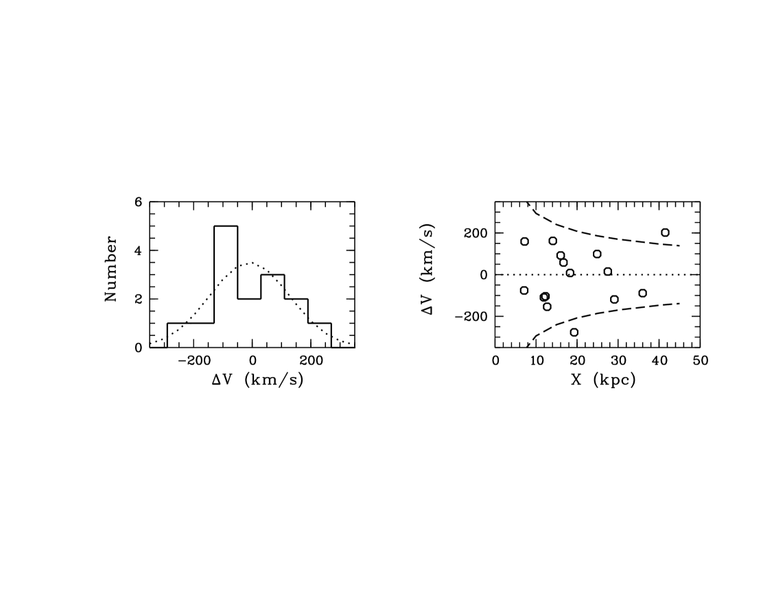
The mean difference between the line-of-sight velocities of the galaxies and their satellites is $\langle\Delta V\rangle$ =–9 $\pm$ 35 km/s. The absolute value of this difference, i.e., the difference with no sign, is 115 $\pm$ 18 km/s. The relatively low values of $\Delta V$ suggest that all objects of our sample are physical pairs. Remarkably, the mean absolute value of the velocity difference for M 51-type galaxies is close to that (137 $\pm$ 6 km/s) for 487 galaxy pairs from the catalog of Karachentsev (1987) with a ratio of the orbital mass of the pair to the total luminosity of its components $f<100$ . Note also that the measurement error of $\Delta V$ in Klimanov et al. (2002) is, on average, only 20 km/s.

Figure 1 (left panel) shows the observed $\Delta V$ distribution. To a first approximation, this distribution can be described by a Gaussian with the standard deviation $\sigma$ =140 km/s (dotted line). Right panel of Fig. 1 shows a plot of the difference $\Delta V$ against the projected linear separation between the main galaxy and its satellite. The dashed lines in the figure represent the expected (Keplerian) dependences for a point mass with M_tot=2 $\times$ 10¹¹ M_⊙ located at the center of the system.

Let us compare the mean values of the individual and orbitalmass estimates for M 51-type galaxies. For a sample of binary galaxies with the plane of the circular orbit randomly oriented relative to the line of sight, the total mass of the components can be found as M_orb=(32/3 $\pi$ )(X $\Delta V^{2}/G$ ), where $G$ is the gravitational constant (Karachentsev 1987). For the objects of our sample, $\langle$ M_orb $\rangle$ =(2.9 $\pm$ 1.0) $\times$ 10¹¹ M_⊙. We will determine the individual masses of the main components by using the maximum rotation velocities (see the next section) and by assuming that the rotation curves of the galaxies within their optical radii are flat. For a spherical distribution of matter, we then obtain the mean mass of the main galaxy, $\langle$ M_main $\rangle$ =(1.6 $\pm$ 0.4) $\times$ 10¹¹ M_⊙, and the mass-to-luminosity ratio, $\langle$ M ${}_{main}/L_{main}(B)\rangle$ =4.7 $\pm$ 0.9 M_⊙/ $L_{\odot,B}$ . The ratio of the orbital mass of M 51-type systems to the mass of the main galaxy for the objects under consideration is 1.9 $\pm$ 0.5. Given the satellite’s mass, the ratio of the orbital mass of the system to the total mass of the two galaxies is $\approx$ 1.6 (for a fixed mass-to-luminosity ratio and a mean luminosity ratio of the satellite and the main galaxy equal to 0.16). If the orbits of the satellites are assumed to be not circular but elliptical with the mean eccentricity $e$ =0.7 (Ghigna et al. 1998), then the orbital mass estimate increases by a factor of 1.5 (Karachentsev 1987). The ratio of the orbital mass of the system to the total mass of the two galaxies also increases by a factor of 1.5 (to 2.4). Consequently, we obtained evidence for the existence of moderately massive dark halos around bright spiral galaxies within (1.5–2)R₂₅.

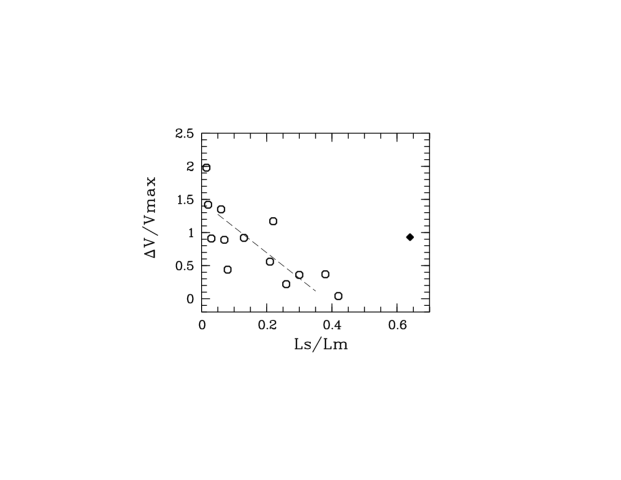
In Fig. 2, $k=|\Delta V|/V_{max}$ is plotted against the ratio of the observed $B$ -band luminosities of the satellite and the main galaxy ( $L_{s}/L_{m}$ ), where $V_{max}$ is the maximum rotation velocity of the main galaxy. If $|\Delta V|/V_{max}$ is close to unity, then the relative velocity of the satellite is approximately equal to the disk rotation velocity of the main galaxy; if $k\approx$ 0, then the satellite’s observed velocity is close to the velocity of the main galaxy. We see a clear trend in the figure – relatively more massive satellites show lower values of $k$ . If we restrict our analysis to satellites with $L_{s}/L_{m}<0.5$ (circles), then the correlation coefficient of the dependence shown in Fig. 2 is -0.77; i.e., the correlation is statistically significant at $P>$ 99% (the diamond in the figure indicates the parameters of the system NGC 3808A,B with $L_{s}/L_{m}$ =0.64.) The corresponding linear fit is indicated in the figure by the dashed straight line. Low-mass satellites with $L_{s}/L_{m}<0.2$ are located, on average, on the extension of the rotation curve for the main galaxy and have velocities close to $V_{max}$ (for them, $\langle k\rangle=1.13\pm 0.19$ ). More massive satellites with $0.2<L_{s}/L_{m}<0.5$ have a lower relative velocity: $\langle k\rangle=0.52\pm 0.15$ .

There is another curious trend: more distant satellites are, on average, more massive. This trend can be explained by observational selection when choosing candidates for M 51-type galaxies. Another plausible explanation is that the massive satellites located near the main galaxy have a shorter evolution scale, because the characteristic lifetime of a satellite near a massive galaxy due to dynamical friction is inversely proportional to the satellite’s mass (Binney and Tremaine 1987).

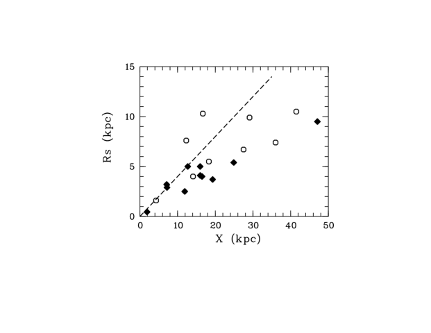
The optical radius of the satellite is plotted against the projected linear distance to the center of the main galaxy in Fig. 3. The dashed straight line in the figure indicates the expected tidal radius of the satellite as a function of the distance to the point mass (Binney and Tremaine 1987); the mass ratio of the satellite and the main galaxy was taken to be 1/3 (this was done in accordance with our formal criterion for classifying a system as being of the M 51 type (see the Introduction). As we see from the figure, in general, the satellites satisfy the tidal constraint imposed on their sizes. Moreover, the relatively more (circles) and less (diamonds) massive satellites show steeper and flatter dependences, respectively. If the satellite’s size is limited by the tidal effect of the main component, then this is to be expected, because the tidal radius is roughly proportional to (M_s/M_m)^1/3, where M_s/M_m is the mass ratio of the satellite and the main galaxy (Binney and Tremaine 1987).

In ten of the twelve binary systems whose observations are presented in Klimanov et al. (2002), the satellite moves relative to the dynamical center of the main component in the same direction as the direction of rotation of the part of the main galaxy’s disk facing it. In two cases (NGC 2535/36 and NGC 4137), the motion of the satellite may be retrograde, although both main galaxies in these systems are seen almost face-on and this conclusion is preliminary.

3 The Tully–Fisher relation

The relation between luminosity and rotation velocity (the Tully–Fisher (TF) relation) is one of the most fundamental correlations for spiral galaxies. This relation is widely used to study the large-scale spatial distribution of galaxies. In addition, it is an important test for the various kinds of models that describe the formation and evolution of spiral galaxies.

The observed rotation curves of M 51-type galaxies are often highly irregular (see Fig. 1 in Klimanov et al. 2002). Therefore, to estimate the maximum rotation velocity, we used the empirical fit to the rotation curve suggested by Courteau (1997):

$v(r)=v_{0}+v_{c}\,(1+x)^{\beta}(1+x^{\gamma})^{-1/\gamma}$ ,

where $r$ is the distance from the dynamical center, $v_{0}$ is the line-of-sight velocity of the dynamical center, $v_{c}$ is the asymptotic rotation velocity, and $x=r_{t}/r$ ( $\beta$ , $\gamma$ , and $r_{t}$ are the parameters). This formula well represents the rotation curves for most spiral galaxies (Courteau 1997).

Figure 4 shows the distribution of the parameters of M 51-type galaxies in the absolute magnitude ( $M(B)$ )-maximum rotation velocity ( $V_{max}$ ) plane. The values of $M(B)$ for the sample objects were corrected for internal extinction, as prescribed by the LEDA database. We took the values of $v_{c}$ (see above) obtained by fitting the observed rotation curves as the maximum rotation velocity for most objects. In addition, these values were corrected in a standard way for the disk inclination to the line of sight and for the deviation of the spectrograph slit position from the galaxy’s major axis. For eight galaxies, we estimated $V_{max}$ from the LEDA HI line widths.

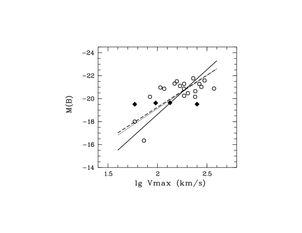
As we see from Fig. 4, the parameters of M 51-type galaxies are located along a flatter relation than are those of nearby spiral galaxies. The mean relation for the objects of our sample indicated by the dashed straight line is $L(B)\propto V_{max}^{-(2.2\pm 0.6)}$ , while the relation for local field spiral galaxies is $L(B)\propto V_{max}^{-(3.1\div 3.2)}$ (Tully et al. 1998; Sakai et al. 2000). The bright (massive) binary members are located near the standard relation (Fig. 4). This location is consistent with the conclusion that the TF relation for giant spiral galaxies does not depend on their spatial environment (Evstigneeva and Reshetnikov 2001). The M 51-type galaxies with $V_{max}\leq 150$ km/s lie, on average, above the relation for single galaxies and, at a fixed $V_{max}$ , show a higher luminosity (or, conversely, at the same luminosity, they are characterized by, on average, lower observed values of $V_{max}$ ).

A similar fact (a different TF relation for the members of interacting galaxy systems and an excess luminosity of the low-mass members of these systems) was, probably, first pointed out by Reshetnikov (1994). The members of close pairs of galaxies also exhibit a flatter TF relation: $L(R)\propto V_{max}^{-2.2}$ (Barton et al. 2001). Barton et al. (2001) argue that interaction-triggered violent star formation in galaxies could be mainly responsible for the different slope of the TF relation for the binary members. Starbursts more strongly affect the observed luminosities of the low-mass galaxies by taking them away from the standard TF relation.

Violent star formation appears to be also responsible for the flatter TF relation for M 51-type galaxies. As we showed previously (Klimanov and Reshetnikov 2001), IRAS data on the far-infrared radiation from galaxies suggest an enhanced star formation rate in M 51-type systems compared to local field objects. Unfortunately, the IRAS angular resolution is too low to separate the contributions from the main galaxy and its satellite to the observed radiation. Figure 4 provides circumstantial evidence for violent star formation in both binary components.

Interestingly, a flatter TF relation has also been recently found (Ziegler et al. 2002) for spiral galaxies at redshifts $z\sim 0.5$ (see Fig. 4). The similarity between the TF relations for nearby interacting/binary galaxies and distant spirals suggests that violent star formation triggered by interaction (mergers) could be responsible for the observed luminosity evolution in distant low-mass galaxies. The rate of interactions and mergers between galaxies rapidly increases toward $z\sim 1$ (Le Fevre et al. 2000; Reshetnikov 2000). This mechanism must undoubtedly contribute to the luminosity evolution and, hence, to the observed TF relation.

4 The evolution of the frequency of occurrence of M 51-type galaxies

Let us consider how the space density of M 51-type galaxies changes with increasing redshift $z$ . To this end, we studied the original frames of the Northern and Southern Hubble Deep Fields (Ferguson et al. 2000) and selected candidates for distant objects of this type. In selecting objects, we used the same criteria as those used to make the sample of nearby galaxies. Unfortunately, there are no published spectroscopic $z$ estimates simultaneously for the main galaxy and for its satellite for any of the systems.

Each of the Deep Fields contains several thousand galaxies; the images of many of them are seen in projection closely or superimposed on one another, which makes it difficult to select candidates for M 51-type objects. Therefore, we restricted our analysis only to relatively bright and nearby galaxies ( $z<1.1$ ).

The candidates for distant M 51-type objects are listed in the Table 1. The first column of the table gives the galaxy name from the catalog of Fernandez-Soto et al. (1999) (the first four and last three objects are located in the Northern and Southern Fields, respectively); the second column gives the galaxy’s apparent magnitude in the HST $I_{814}$ filter (for the first two systems, we took the estimates from the catalog of Fernandez-Soto et al.; for the remaining systems, we provide our own magnitude estimates); the third column gives the redshift (the spectroscopic $z$ estimates (Cohen et al. 2000) are given with three significant figures; the photometric $z$ estimates (Fernandez-Soto et al. 1999) are marked by a colon); the fourth column gives the spectral type, which characterizes the galaxy’s spectral energy distribution (Fernandez-Soto et al. 1999); and the last column contains our measurements of the angular separation between the nuclei of the main galaxy and its satellite.

Table 1: Candidates for M 51-type galaxies in the Hubble Deep Fields

Name	$I_{\rm 814}$	$z$	Spectral	$X$ (^′′)
			type
n45	21.26	1.012	Scd	2.95
n78	25.30	1.04:	Irr
n350	21.27	0.320	Scd	3.36
n351	24.03	0.24:	Irr
n888a	23.88	0.559	Irr	0.72
n888b	25.75
n938a	23.11	0.557	Scd	1.37
n938b	25.85
SB-WF-2033-3411a	22.76	0.55:	Irr	1.44
b	24.94
SB-WF-2736-0920a	22.01	0.59:	Scd	1.54
b	24.30
SB-WF-2782-4400a	23.05	0.53:	Irr	0.89
b	24.58

The integrated parameters of the selected candidates for M 51-type systems are close, within the error limits, to those of nearby systems (see Section 2). Thus, the ratio of the observed luminosities of the satellite and the main galaxy is 0.13 $\pm$ 0.07 (in the $I_{814}$ filter, which roughly corresponds to the $B$ band in the frame of reference associated with the objects themselves at the mean redshift of the sample under consideration); the mean observed separation between the main components and their satellites is 12 $\pm$ 7 kpc. The absolute magnitude of the main galaxies that was estimated by applying the $k$ correction (Lilly et al. 1995) is $M(B)=-19\fm 4\pm 1\fm 4$ . (These values, as well as those given below, were calculated for a cosmological model with a nonzero $\Lambda$ term: $\Omega_{m}$ =0.3, $\Omega_{\Lambda}$ =0.7, H₀=65 km s^-1 Mpc^-1.)

To estimate the evolution rate of the space density of galaxies with $z$ , we use the same approach that was used by Reshetnikov (2000). By assuming that the space density of M 51-type galaxies changes as

$n(z)=n_{0}(1+z)^{m}$

( $n(z)$ is the number of objects per unit volume (Mpc^-3) at redshift $z$ and $n_{0}=n(z=0)$ ), we calculate the expected number of galaxies in the direction of the Deep Fields in the $z$ range concerned for various exponents $m$ .

The most important parameter required for this estimation is the spatial abundance of M 51-type galaxies in a region of the Universe close to us ( $n_{0}$ ). According to Klimanov (2003), M 51-type galaxies account for 0.3% of the field galaxies and about 4% of the binary galaxies. Interestingly, this estimate is close to the frequency of occurrence estimated by Vorontsov-Vel’yaminov (1978), who assumed that M 51-type galaxies accounted for about 10% of the interacting galaxies. Assuming that about 5% of the galaxies are members of interacting systems (Karachentsev and Makarov 1999), we find that M 51-type systems account for 0.5% of all galaxies. By integrating the luminosity function of the field galaxies taken from the SDSS and 2dF surveys (Blanton et al. 2001; Norberg et al. 2002) in the range of absolute magnitudes $M(B)$ from -17^m to -22\fm5, we can estimate the space density of field galaxies in this luminosity range as 0.017 Mpc^-3 and, hence, $n_{0}$ = 5.1 10^-5 Mpc^-3.

Integrating the expression $n_{0}(1+z)^{m}$ over the $z$ range from 0.2 to 1.1, we found that in the absence of density evolution ( $m=0$ ), the expected number of M 51-type galaxies in the two fields is 0.8. The observed number of objects (seven) exceeds their expected number by more than two standard Poisson deviations ( $\sigma=\sqrt{7}=2.65$ ). Despite the poor statistics, this result provides evidence for the evolution of the spatial abundance of M 51-type objects with $z$ . The exponent $m=3.6$ corresponds to the observed number of galaxies. The formal spread in this value that corresponds to the range of the number of objects from $7-\sqrt{7}$ to $7+\sqrt{7}$ is ${}^{+0.5}_{-0.8}$ . The actual error in the $m$ estimate can be much larger, for example, because of the uncertainty in $n_{0}$ .

Of course, the estimated evolution rate depends on the assumed cosmological model. For example, for a flat Universe with a zero $\Lambda$ term and H₀=75 km s^-1 Mpc^-1, the exponent $m$ increases to 4.8.

5 Discussion

A typical M 51-type binary system is a bright spiral galaxy with a relatively low-mass satellite physically associated with it located near the boundary of its disk. In most cases, the satellite shows prograde motion; i.e., it rotates in the same direction as the main galaxy (see Section 2). Observational selection may be responsible for this peculiarity, because the satellite whose direction of orbital motion coincides with the direction of rotation of the main galaxy can excite and maintain a large-scale two-arm pattern on the galactic disk. If the motion of the satellite is retrograde, then the tidal response will be much weaker. The presence of a spiral pattern is one of the criteria for classifying a galaxy as an M 51-type object and three quarters of them show a large-scale two-arm pattern (Klimanov and Reshetnikov 2001). Consequently, the predominance of prograde motions of the satellites in objects with a well-developed two-arm spiral pattern can serve as a confirmation of the tidal nature of the spiral arms in such galaxies.

Other indications of the mutual influence of the galaxies in M 51-type systems include an enhanced star formation rate (as evidenced by the high far-infrared luminosities of the systems (Klimanov and Reshetnikov 2001) and, possibly, by the flatter Tully–Fisher relation (Fig. 4)) and the existence of a tidal constraint on the sizes of the satellites (Fig. 3).

M 51-type binary systems are relatively rare objects. According to Klimanov (2003), only 0.7% of the spiral galaxies in the range of absolute $B$ magnitudes from –16^m to –22^m have a relatively bright satellite near the end of the spiral arm and can be classified as objects of this type.

As was shown in the preceding section, the fraction of M 51 type galaxies increases with redshift. Interestingly, within the error limits, the rate of increase in the relative abundance of these objects ( $m=3.6^{+0.5}_{-0.8}$ ) roughly corresponds to the rate of increase in the number of binary and interacting galaxies. Thus, the fraction of galaxies with tidal features is proportionalto $(1+z)^{m}$ with $m=4\pm 1$ (Reshetnikov 2000); the fractions of merging and binary galaxies evolve with $m=3.4\pm 0.6$ and $m=2.7\pm 0.6$ , respectively (Le Fevre et al. 2000).

Let us now try to describe the possible origin and evolution of M 51-type binary systems. Numerical calculations of the formation of galaxies performed in terms of CDM (cold dark matter) models indicate that galaxies are formed within extended dark halos; many less massive subhalos must be contained within a massive halo (see, e.g., Kauffmann et al. 1993; Klypin et al. 1999). Thus, the halo of a galaxy with a mass comparable to the mass of the Milky Way must include several tens of satellites of different masses within its virial radius of 200–300 kpc (Benson et al. 2002a). Numerical calculations suggest that $\leq$ 5% of the galaxies similar to the Milky Way have satellites with a $V$ -band luminosity of –18^m (Benson et al. 2002b). Consequently, such satellites (their luminosity is typical of the satellites of M 51-type objects) are relatively but not extremely rare. Recall that our Galaxy has such a satellite, the Large Magellanic Cloud, at a distance of about 50 kpc.

What is the subsequent fate of the relatively massive satellites formed in the halos of galaxies similar to the Milky Way? The evolution of the satellites will be governed mainly by two processes: (1) dynamical friction, which will cause the satellite’s orbital decay until the satellite merges with the main component; and (2) tidal stripping, which causes a decrease in the satellite’s mass and, as a result, an increase in the lifetime of its separate existence from the main galaxy. Recent studies suggest that the lifetime of a satellite under dynamical friction can be much longer than assumed previously (see, e.g., Colpi et al. 1999; Hashimoto et al. 2003). In addition, this lifetime depends weakly on the orbital eccentricity of the satellite (Colpi et al. 1999).

Cosmological calculations indicate that the satellites formed within the massive halo of a central object are in highly elongated orbits with a mean eccentricity of $e=0.6-0.8$ (Ghigna et al. 1998). If such satellites are assumed to be observed in M 51-type systems mostly near the orbital pericenter (in this case, their tidal effect on the disk of the main galaxy is at a maximum), i.e., $r_{p}=24$ kpc, then the distance at the apocenter is 100–150 kpc and the orbital period of the satellite is 3–6 Gyr. In the Hubble time, such a satellite would make only 2 to 4 turns and might not be absorbed by the central galaxy by $z=0$ . During its first encounter with the main galaxy, the satellite can lose 50% of its mass, which significantly increases the time of its orbital evolution (Colpi et al. 1999). Consequently, the “cosmological” satellites formed on the periphery of the halos of central galaxies could in several cases survive by $z=0$ and be currently observed together with the main components as M 51-type binary systems.

Another, apparently more realistic scenario for the formation of the binary systems under consideration is the capture of a relatively low-mass object by a central galaxy during their chance encounter. At present, the interactions of galaxies are relatively rare events, but they are observed more and more often with increasing $z$ (at least up to $z\approx 1$ ). Whereas only $\approx$ 5% of the galaxies at $z=0$ are members of interacting systems with clear morphological evidence of perturbation (Karachentsev and Makarov 1999), this fraction at $z=1$ is $\approx$ 50% (Reshetnikov 2000; Le Fevre et al. 2000). Thus, an event during which a massive galaxy at $z\geq 0.5$ captures a satellite seems quite likely. This event is all the more likely since the peculiar velocities of the galaxies were earlier lower and, hence, their chance encounters occurred with lower relative velocities and more often led to the formation of bound systems or mergers (see, e.g., Balland et al. 1998). The orbital period in a circular orbit with a semimajor axis of $a=24$ kpc around a galaxy similar to the Milky Way is 0.5–1 Gyr. Consequently, in several Gyr (recall that an age equal to about half of the Hubble time corresponds to $z=1$ ), most of such satellites will be absorbed by the main galaxies (Colpi et al. 1999; Penarrubia et al. 2002); by the time that corresponds to $z=0$ , they must be observed rarely. This scenario is confirmed by our evidence for the relatively rapid evolution of the space density of M 51-type objects with $z$ .

Thus, the currently observed M 51-type systems could have both a primordial origin and a more recent origin – through the capture of a satellite by the main galaxy. Mixed scenarios are also possible, for example, when an encounter with another galaxy can change the orbit of the peripheral satellite and push it closer to the main galaxy. Of course, the actual pattern of formation and evolution of the binary systems under consideration is much more complex, and it should be tested by numerical calculations.

How does the galaxy M 51, the prototype of this class of objects, fit into the scenarios described above? It should be noted that in some respects, this binary system is not a typical representative of the M 51-type systems. For example, the mass ratio of the satellite and the main galaxy for it is 1/3 or even 1/2, a value that is larger than that for a typical binary system of this type. The dynamical structure of the binary system is not completely understood either. The apparent morphology and kinematics of M 51 can be explained both in terms of the models according to which we observe the separation of the galaxies after their first encounter (Durrell et al. 2003) and in terms of the approach according to which multiple encounters of the satellite and the main galaxy have already taken place in this system (Salo and Laurikainen 2000). In the former case, the system M 51 has, probably, formed recently (we observe it several hundred Myr after the passage of the satellite through the pericenter) during a close encounter of the galaxies NGC 5194 and NGC 5195; in the latter case, this system is much older and its age can reach several Gyr.

In conclusion, note that because of the relatively small number of systems studied, some of our results (a different slope of the TF relation and an increase in the frequency of occurrence of M 51-type galaxies with $z$ ) are preliminary and should be confirmed using more extensive observational data.

Acknowledgments

This study was supported by the Federal Program “Astronomy” (project no. 40.022.1.1.1101).

REFERENCES

1. Ch. Balland, J. Silk, and R. Schaeffer, Astrophys. J. 497, 541 (1998).

2. E. J. Barton, M. J. Geller, B. C. Bromley, et al., Astron. J. 121, 625 (2001).

3. A. J. Benson, C. G. Lacey, C. M. Baugh, et al., Mon. Not. R. Astron. Soc. 333, 156 (2002a).

4. A. J. Benson, C. S. Frenk, C. G. Lacey, et al., Mon. Not. R. Astron. Soc. 333, 177 (2002b).

5. J. Binney and S. Tremaine, Galactic Dynamics (Cambridge University Press, Princeton, 1987).

6. M. R. Blanton, J. Dalcanton, D. Eisenstein, et al., Astron. J. 121, 2358 (2001).

7. J. G. Cohen, D. W. Hogg, R. Blandford, et al., Astrophys. J. 538, 29 (2000).

8. M. Colpi, L. Mayer, and F. Governato, Astrophys. J. 525, 720 (1999).

9. S. Courteau, Astron. J. 114, 2402 (1997).

10. P. R. Durrell, J. Ch.Mihos, J. J. Feldmeier, et al., Astrophys. J. 582, 170 (2003).

11. E. A. Evstigneeva and V. P. Reshetnikov, Astrofizika 44, 193, 2001.

12. H. C. Ferguson, M. Dickinson, and R. Williams, Ann. Rev. Astron. Astrophys. 38, 667 (2000).

13. A. Fernandez-Soto, K. M. Lanzetta, and A. Yahil, Astrophys. J. 513, 34 (1999).

14. S. Ghigna, B. Moore, F. Governato, et al., Mon. Not. R. Astron. Soc. 300, 146 (1998).

15. Y. Hashimoto, Y. Funato, and J. Makino, Astrophys. J. 582, 196 (2003).

16. I. D. Karachentsev, Binary Galaxies (Nauka, Moscow, 1987).

17. I. D. Karachentsev, D. I. Makarov, Galaxy Interactions at Low and High Redshift Ed. by J. E. Barnes and D. B. Sanders (1999), p. 109.

18. G. Kauffmann, S. D.M. White, and B. Guiderdoni, Mon. Not. R. Astron. Soc. 264, 201, 1993.

19. S. A. Klimanov, Astrofizika 46, 191 (2003).

20. S. A. Klimanov and V. P. Reshetnikov, Astron. Astrophys. 378, 428 (2001).

21. S. A. Klimanov, V. P. Reshetnikov, and A. N. Burenkov, Pis’ma Astron. Zh. 28, 643 (2002) [Astron. Lett. 28, 579 (2002)].

22. A. Klypin, A. V. Kravtsov, O. Valenzuela, and F. Prada, Astrophys. J. 522, 82 (1999).

23. O. Le Fevre, R. Abraham, S. J. Lilly, et al., Mon. Not. R. Astron. Soc. 311, 565 (2000).

24. S. J. Lilly, L. Tresse, F. Hammer, et al., Astrophys. J. 455, 108 (1995).

25. P. Norberg, Sh.Cole, C. M. Baugh, et al., Mon. Not. R. Astron. Soc. 336, 907 (2002).

26. J. Penarrubia, P. Kroupa, and Ch.M. Boily, Mon. Not. R. Astron. Soc. 333, 779 (2002).

27. V. P. Reshetnikov, Astrophys. Space. Sci. 211, 155 (1994).

28. V. P. Reshetnikov, Astron. Astrophys. 353, 92 (2000).

29. S. Sakai, J. R. Mould, S. M.G. Hughes, et al., Astrophys. J. 529, 698 (2000).

30. H. Salo and E. Laurikainen, Mon. Not. R. Astron. Soc. 319, 377 (2000).

31. R. B. Tully, M. J. Pierce, J.-Sh.Huang, et al., Astron. J. 115, 2264 (1998).

32. B. A. Vorontsov-Vel’yaminov, Astron. Zh. 52, 692 (1975) [Sov. Astron. Rep. 19, 422 (1975)].

33. B. A. Vorontsov-Vel’yaminov, A. A. Krasnogorskaya, and V. P. Arkhipova, A Morphological Catalog of Galaxies (Izd. Mos. Gos. Univ., Moscow, 1962–1968), v. 1–4.

34. B.A. Vorontsov-Vel’yaminov, Exragalactic Astronomy (Nauka, Moscow, 1978).

35. B. L. Ziegler, A. Bohm, K. J. Fricker, et al., Astrophys. J. 564, L69 (2002).