Integration of the atmospheric fluctuations in a dual-field optical interferometer: the short exposure regime

Spatial phase-referencing in dual-field optical interferometry is reconsidered. Our analysis is based on the 2-sample variance of the differential phase between target and reference star. We show that averaging over time of the atmospheric effects depends on this 2-sample phase variance (Allan variance) rather than on the true variance. The proper expression for fringe smearing beyond the isoplanatic angle is derived. With simulations of atmospheric effects, based on a Paranal turbulence model, we show how the performances of a dual-field optical interferometer can be evaluated in a diagram ’separation angle’ versus ’magnitude of faint object’. In this diagram, a domain with short exposure is found to be most useful for interferometry, with about the same magnitude limits in the $H$ and $K$ bands. With star counts from a Galaxy model, we evaluate the sky coverage for differential astrometry and detection of exoplanets, i.e. likelihood of faint reference stars in the vicinity of a bright target. With the 2mass survey, we evaluate sky coverage for phase-referencing, i.e. avaibility of a bright enough star for main delay tracking in the vicinity of any target direction.

1 Introduction

Phase-referencing in ground-based optical interferometry has been proposed for faint object imaging, for narrow-angle astrometry and for improved precisions in visibility measurements (Mozurkewich et al. (1988); Colavita (1992); Quirrenbach et al. (1994)). Phase-referencing is the interferometer counterpart of Adaptive Optics (AO) developed for single-pupils. Inhomogeneities in the atmosphere cause the optical path difference (OPD) between two telescopes to fluctuate over a range of time scales, from a few milliseconds upwards, with variance rms of about 10 $\mu$m. These fluctuations can be measured continuously on a bright star and used to track a faint star in the immediate surrounding. Then faint objects can be observed and small visibility amplitude measured with sufficient Signal/Noise ratio. Furthermore, differential OPD fluctuations ($\Delta$OPD) between target and reference stars should average out over long integrations, leading to differential phase structure for faint objects partially resolved, or to high precision astrometry for unresolved sources.

It has been noticed that $\Delta$OPD residuals over long integrations are proportional to the measured angle (Shao & Colavita (1992)), so that high precision narrow-angle astrometry needs to be performed with reference sources in the immediate surrounding of the source target, i.e. within the isoplanatic patch. Angular anisoplanatism in optical interferometry has been recently investigated (Esposito et al. (2000)). The authors define an “isopistonic” angle where the interferometric $\Delta$OPD (rms value) remains smaller than a tenth of the observed wavelength. Their analysis is based on the true variance of differential piston. A detailed analysis of the $\Delta$OPD spectrum has been performed by d’Arcio (1999) who considers also its jitter on short exposures, but does not investigate its potential use in phase-referencing.

With the condition “differential phase rms smaller than 1 radian”, the half-cone angle of Spatial Phase-Referencing (SPR) is found to be the isoplanatic angle for AO (Fried (1982)), divided by ($2^{3/5}$) due to the two entrance pupils of a long baseline interferometer with uncorrelated phase corrugations (Colavita (1992)). Taking into account the aperture size, differential phase excursion remains bounded even on separation angles exceeding slightly the AO isoplanatic angle, and SPR with long integrations is possible. On larger angular separations, random walk of differential phase fluctuations prevents long term averaging. The measurement of differential piston variations is still possible, but with short integrations, shorter than some coherence time for $\Delta$OPD fluctuations. Sensitivity is reduced as compared to small angles, but the chance of finding a bright enough star for phase-referencing is increased. Altogether, SPR in optical interferometry has to be investigated in the whole telescope Field-of-View, that is within a few arcminutes.

An optimization of SPR requires a detailed analysis of the temporal behaviour of differential phase. Our analysis is based on the 2-sample (or Allan) variance of time series of the measured differential phase. This quantity tells us how $\Delta$OPD variations can be recovered before being averaged. Ultimately, the true $\Delta$OPD variance will give the achievable precision on long integrations.

Here we disentangle the problem between differential piston fluctuations and single-pupil wavefront distortion, that is between the first mode and higher modes in the Zernike expansion of phase corrugations. With large apertures, each pupil AO should correct for a wide field of view, with significant gain in the faint source direction.

The $\Delta$OPD model of our analysis is presented in the next Section, and quantities relevant to phase-referencing are recalled and clarified: the 2-sample variance and the attenuation factor due to fringe smearing. Results of numerical simulations are given in Sect. 3, with application to the 1.8m and 8m telescopes at Paranal. We further discuss the optimization of exposure duration and its dependence on faint star magnitude and separation angle (Sect. 4). Different regimes of phase-referencing are outlined in Sect. 5, together with sky coverages.

2 Model for phase-referencing

2.1 Power spectra of atmospheric turbulence

A detailed analysis of power spectra of quantities relevant to optical interferometry can be found in Conan (2000), where various analytical forms are also proposed for integrals of power spectra. In this Section, we recall the main expressions.

The atmospheric turbulence, assumed to be stratified with altitude, is described by a distribution of discrete turbulence layers. The strength of each layer $k$ is characterized by an optical turbulence factor ${\cal J}_{k}$, sum of the refractive index structure parameter $C^{2}_{N}(h)$ along the line of sight through this layer. The power spectrum of atmospheric piston over a single aperture, from a single turbulence layer, with a von Karman turbulence spectrum and outer scale $L_{0}$, is:

$$W_{P}({\bf f})=0.00969\,(f^{2}+f^{2}_{0})^{-11/6}\,{\cal J}_{k}\,F_{D}(f)$$ (1)

where $f_{0}=1/L_{0}$, and $F_{D}(f)$ is the spatial filter due to finite aperture size, and
$F_{D}(f)\,=\,[2J_{1}(\pi Df)/\pi Df]^{2}$ for a filled circular aperture with diameter $D$.

For two sources at angular distance $\Theta$, and a turbulent layer at distance $h$ along the line of sight, the power spectrum of differential piston over a single aperture is obtained from the covariance function:

$$W_{\Delta P}({\bf f})=2W_{P}({\bf f})(1-\cos(2\pi{\bf f}\cdot{\bf R}))$$ (2)

with ${\bf R}=h$$\Theta$.
Similarly, the power spectrum of interferometric piston or OPD, with a baseline ${\bf B}$ is:

$$W_{OPD}({\bf f})=2W_{P}({\bf f})(1-\cos(2\pi{\bf f}\cdot{\bf B}))$$ (3)

and the power spectrum of differential interferometric piston ($\Delta$OPD) is obtained with the product of the two filter functions:

$$W_{\Delta OPD}({\bf f})=4W_{P}({\bf f})(1-\cos(2\pi{\bf f}\cdot{\bf R}))(1-\cos(2\pi{\bf f}\cdot{\bf B}))$$ (4)

With the Taylor hypothesis, turbulence is displacing as a whole with velocity ${\bf V}_{k}$ in the turbulent layer $k$. In each layer, we take the $x$-direction along the wind direction (${\bf f\cdot V}_{k}=f_{x}V_{k}$). The temporal power spectrum of frequency $\nu$ is, for that layer:

$$w_{k}(\nu)=\frac{1}{V_{k}}\int_{-\infty}^{\infty}W_{k}(\frac{\nu}{V_{k}},f_{y})df_{y}$$ (5)

The temporal power spectra of independent contributions are summed together giving the total power spectrum ${\cal W}(\nu)$ of $\Delta$OPD, for the whole atmosphere crossing.

2.2 Relevant quantities in phase-referencing

In the following, we consider that the main OPD is tracked exactly on a bright star and does not contribute to interferometric noise. The ability to follow $\Delta$OPD with time, i.e. to measure its variation from one sample to the next, is a critical issue in case of large phase excursion, i.e. for angular separation larger than some “isopistonic” angle. Indeed, sample phase measurements have to be unwrapped for long term averaging of the differential piston. The relevant physical quantity is not so much the magnitude of differential phase (due to differential piston), but each sample departure from a local average. The most useful quantity for describing such a process is the 2-sample variance, or Allan variance used for the characterisation of frequency standards (Rutman (1978)). The local average is simply made with two successive samples. Let $\tau_{0}$ be the exposure duration for each sample $\Delta\mathrm{OPD}_{i}$, and also the sampling interval. The 2-sample variance of the time series is $\sigma^{2}_{A}(\tau_{0})=\,\frac{1}{2}\,\langle(\Delta\mathrm{OPD}_{i+1}-\Delta\mathrm{OPD}_{i})^{2}\rangle$, and it can be expressed in terms of the true variance $I^{2}_{\Delta OPD}(\tau)$ by (Rutman (1978)):

$$\sigma^{2}_{A}(\tau_{0})\,=\,2[I^{2}_{\Delta OPD}(\tau_{0})-I^{2}_{\Delta OPD}(2\tau_{0})]$$ (6)

with:

$$I^{2}_{\Delta OPD}(\tau)\,=\,2\int_{0}^{\infty}{\cal W}(\nu)[\frac{\sin(\pi\nu\tau)}{\pi\nu\tau}]^{2}d\nu$$ (7)

A third relevant quantity is the phase jitter within each sample, responsible for fringe smearing and then signal loss. A detailed analysis of fringe smearing in VLBI, due to instabilities in frequency oscillators, can be found in Thompson et al. (2001). A similar approach applied to differential piston in dual-field optical interferometry yields the following expression for the attenuation factor due to finite exposure duration.

Let $\Delta\phi(t)$ be the differential interferometric phase (due to $\Delta$OPD), and $\tau_{0}$ the exposure duration. The (random) attenuation factor $g_{i}$ and measured differential phase $\Delta\phi_{i}$ are given by:

$$g_{i}e^{j\Delta\phi_{i}}\,=\,\frac{1}{\tau_{0}}\int_{t_{i}}^{t_{i}+\tau_{0}}e^{j\Delta\phi(t)}dt$$ (8)

With a quadrature-phase scheme for fringe phase and amplitude measurements, the average attenuation factor useful for Signal/Noise ratio estimate, $G(\tau_{0})$, is taken as the square root of the quadratic average of $g_{i}$:

$$G(\tau_{0})\,=\,\Big{[}\frac{1}{\tau_{0}^{2}}\int_{0}^{\tau_{0}}\int_{0}^{\tau_{0}}\langle\exp j[\Delta\phi(t)-\Delta\phi(t^{\prime})]\rangle dtdt^{\prime}\Big{]}^{1/2}$$ (9)

If $\Delta\phi$ has gaussian statistics and is a stationary process, the quantity between brackets is expressed in terms of the structure function of differential interferometric phase: $\sigma^{2}_{\Delta\phi}(\tau)\,=\,2\,(\frac{2\pi}{\lambda})^{2}[R(0)-R(\tau)]$, where $\lambda$ is the optical wavelength, and $R(\tau)$ the correlation function or Fourier Transform of ${\cal W}(\nu)$:

$$R(\tau)\,=\,2\int_{0}^{\infty}{\cal W}(\nu)\cos(2\pi\nu\tau)d\nu$$ (10)

Equ. 9 is now written:

$$G(\tau_{0})\,=\,\Big{[}\frac{2}{\tau_{0}}\int_{0}^{\tau_{0}}(1-\frac{t}{\tau_{0}})\exp(-\frac{\sigma^{2}_{\Delta\phi}(t)}{2})dt\Big{]}^{1/2}$$ (11)

A similar expression is given by Buscher (buscher88 (1988)) for the smearing factor on main OPD, the fringe correlation function $\exp(-\frac{\sigma^{2}_{\Delta\phi}(t)}{2})$ being expressed in terms of an interferometer coherence time. In previous works on off-axis phase-referencing, the fringe smearing factor has been often approximated by $\exp(-2\pi^{2}\,\sigma^{2}_{res}(\tau_{0})\,/\lambda^{2})$, where $\sigma^{2}_{res}(\tau_{0})=2\int_{0}^{\infty}{\cal W}(\nu)[1-{\rm sinc}(\pi\nu\tau)]^{2}d\nu$, valid only in the weak smearing limit, that is useless for phase-referencing beyond the “isopistonic” angle.

2.3 Turbulence model of the atmosphere

Distribution profile of turbulence parameters above Paranal are taken from the results of the PARSCA campaign of March 1992 (Fuchs & Vernin (1993)), with balloon soundings and SCIDAR measurements. The average turbulence profile [$C_{n}^{2}(h)$] and wind amplitude profile [$V(h)$] have been used by several authors for simulations of atmospheric effects (Delplancke et al. (2000); Esposito et al. (2000)), with a nominal seeing of 0.65”. Continuous profiles from the PARSCA report have been re-sampled with 1 km step (which is about the vertical resolution of SCIDAR measurements). Turbulence content summed over each layer is the optical turbulence factor ${\cal J}_{k}$ used in the following. Wind velocity has also been averaged over each layer and is shown on Fig. 1. In this model, the weighted average wind velocity equals 8.5m/s.

Figure 1: Distribution of turbulence parameters with altitude above Paranal, from the average model of PARSCA 1992 campaign. The turbulence factor is in $m^{1/3}$. The 15 layers adopted in our model are marked with triangles.

Wind direction is another useful parameter but is not available in the report on the PARSCA campaign. Wind direction changes somehow with altitude, and scatter in wind direction smoothes singularities of the “frozen in” turbulence model. We have taken a dominant wind direction mainly perpendicular to the interferometer baseline, that is a situation where turbulence effects in long baseline interferometry are the most significant.

Another parameter of the model is the outer scale of turbulence in each one of the layers ($L_{0,k}$). This quantity is hardly measured locally. The Generalized Seeing Monitor (GSM) can measure a weighted average of $L_{0,k}$ along the line of sight. Strong turbulence layers with small $L_{0}$ values have a dominant effect in this weighted average (Borgnino (1990)). The spatial coherence outer scale measured in this way at Paranal has a log-normal distribution with a median value of 22m (Martin et al. (2000)) which may reflect mainly turbulence properties close to the telescope. The outer scale high in the atmosphere has a significant impact on long term averaging, and a limited impact on short term averaging of differential phase, as shown in the next Section. So, the lack of a detailed knowledge of the outer scale distribution with altitude does not impinge on our study.

3 Averaging of atmospheric effects: impacts of separation angle and outer scale

Figure 2: Main OPD variance, and $\Delta$OPD variance for separation angles 15”, 30” and 60”, 100m interferometer baseline and 8m aperture diameter. True variance and 2-sample variance are respectively shown with thin and thick lines. The other parameter is the outer scale of turbulence: 50m (dashed lines), 100m (full lines) and 250m (dash-point lines). For 30” angular separation, only the full line is shown for clarity of the Figure.

Simulations of atmospheric turbulence have been performed with an interferometer baseline of 100m and telescope diameters of 8m and 1.8m. In our model, the separation vector between the two stars is parallel to the baseline direction, and the zenithal distance is nearly zero. The power spectral densities (main OPD and $\Delta$OPD) for each one of the 15 turbulent layers of Fig. 1 are estimated with Equ. 3-5, then the true variance and 2-sample variance, summed on the whole line of sight, are estimated with Equ. 6-7 for different exposure durations $\tau$. Results are shown in Fig. 2, both for main OPD and for $\Delta$OPD. Impacts of separation angles $\theta$ ranging from 15 to 60” and of outer scale $L_{0}$ between 50 and 250 m are shown. For short exposures ($\tau\leq$ a few 0.1 s), differential phase variations, from one sample to the next, is small enough at optical wavelength to allow reconstruction of a continuous and unambiguous differential phase solution from successive samples. The relevant quantity for differential phase reconstruction is then the 2-sample variance, and not the true variance. This difference is essential since the true variance is a monotonic decreasing function with exposure duration whereas the two-sample variance increases first, then peaks at $\tau_{max}\simeq$ 1-2 seconds, and ultimately approaches the true variance for long exposures.

In Fig. 2, the variance is found to be proportional to the square of the angular separation, as already shown with analytic expressions (Shao & Colavita (1992); Colavita (1994)). We point also that:

• the outer scale of turbulence has a significant impact both on main OPD, and on $\Delta$OPD for long exposures, and a small impact on the 2-sample variance for short exposures,

• the variance of $\Delta$OPD remains smaller than 1$\mu$m rms, or much smaller than the coherence length of starlight in the near-IR (with less than 10% relative bandwidth). This makes it possible differential delay tracking without feedback, that is open loop operation whatever the separation angle and exposure duration.

Table 1: Greenwood time delay $t_{0}$, isoplanatic angle $\theta_{0}$, and “isopistonic” angle $\theta_{1}$ for 1.8m (AT) and 8m (UT) telescopes in the $H$ and $K$ band, at zenith, at Paranal.

IR band $$H$$

[ms] 20 29

8.6” 12.1”

10.7” 14.3”

17.4” 23.0”

The Greenwood (or AO) time delay is $t_{0}=0.314\,r_{0}/\bar{V}$ (Fried (1990)), where $r_{0}$ is the Fried parameter and $\bar{V}$ the average wind velocity. For single aperture, the isoplanatic angle $\theta_{0}=[2.91(\frac{2\pi}{\lambda})^{2}\sum_{k}{\cal J}_{k}h_{k}^{5/3}]^{-3/5}$ (Fried (1982)) is defined as the angular extent over which differential wavefront phase corrugations is smaller than 1 radian (rms). By analogy, in interferometry, an angle $\theta_{1}$ can be defined as the angular range where $2\pi\Delta\mathrm{OPD}/\lambda$ (rms value of the true variance) is smaller than 1 radian. The estimation of this parameter is in Table 1 for two different values of telescope diameter and for an outer scale of 100m. The $\theta_{0}$ and $\theta_{1,UT}$ estimates made by Esposito et al. (2000) for the same observing site are somewhat smaller due to a more pessimistic turbulence model and to a more conservative definition of the “isopistonic” angle (rms phase of 2$\pi$/10 instead of 1 rad.).

Figure 3: Smearing factor due to finite exposure duration for differential OPD measurements with separation angles 15”, 30”, 45” and 60”, in the $H$ and $K$ bands (respectively dashed and full lines). The smearing factor is also shown for main OPD measurements.

The average smearing factor $G(\tau_{0})$ given by Equ. 11 is shown in Fig. 3 for $\Delta$OPD measurements with 4 separation angles, from 15 to 60”. This smearing factor in phase-referencing remains close to 1.0 for sample exposure shorter than 0.1s, for the whole range of angular separation. For large enough angles and long exposure duration $\tau$, we verify that the smearing factor is in $\tau^{-1/2}$ as shown by Buscher (buscher88 (1988)).

4 Sensitivity estimates in phase-referencing

Differential piston measurements is affected by the limited Signal/Noise ratio that can be achieved on faint sources. With $\cal B$ and $\cal S$ respectively the noise and signal in visibility measurement of the faint source, the measured 2-sample differential OPD variance is the sum of two contributions, a measurement noise and an atmospheric differential OPD:

$$Y^{2}(\tau_{0})\,=\,\sigma^{2}_{m}(\tau_{0})\,+\,\sigma^{2}_{A}(\tau_{0})$$ (12)

The measurement noise variance, given by:

$$\sigma^{2}_{m}(\tau_{0})\,=\,(\frac{\lambda}{2\pi})^{2}\,(\frac{{\cal B}(\tau_{0})}{{\cal S}(\tau_{0})})^{2}$$ (13)

is a decreasing function of the coherent exposure duration $\tau_{0}$, whereas the 2-sample variance $\sigma^{2}_{A}$ of $\Delta$OPD first increases from zero to its peak value, and then decreases. The quadratic sum of the two often shows a local minimum that gives an optimum exposure duration.

4.1 Signal and Noise

Sensitivity estimate is performed in the $H$ and $K$ bands. Measurement noise contributions are assumed to come from read-out noise of the detector, and from star and background photon noise. Let $\sigma_{l}$ be the read-out noise, in electrons per measurement, $b_{0}$ and $s_{M}$ the number of photons that would be detected per second and per aperture from sky background and from a star with magnitude $M$, respectively, without mode filtering. Fringe phase measurement is supposed to be performed with an ABCD scheme and 4 simultaneous detector readouts, also known as ’spatial discrete modulation scheme with 4 phases’ (Cassaing et al. (2000)). In the photon-rich limit, the Signal and Noise of such a detection scheme have been derived (Daigne & Lestrade (1999)). With additional mode filtering before detection, the source noise contribution is further reduced and we get:

$${\cal S}(\tau_{0})\,=\,\gamma\Gamma G(\tau_{0})s_{M}\tau_{0}$$ (14)

$${\cal B}^{2}(\tau_{0})\,=\,2\sigma_{l}^{2}+(b_{0}+\Gamma s_{M})\tau_{0}$$ (15)

$\gamma$ being the interferometer visibility, $\Gamma$ the average Strehl ratio or aperture efficiency in the point source direction, and $G(\tau_{0})$ the average fringe smearing factor for exposure duration $\tau_{0}$ (Equ. 11). Strehl ratio fluctuations, uncorrelated on the two pupils, are responsible for an additional loss of coherence due to unbalanced amplitudes, which is not considered here.

Parameters of SNR estimates for the UTs are given in Table 2. The overall photometric efficiency is the arm transmission factor (0.30 and 0.31 in the $H$ and $K$ band respectively) times additional factors: coude train with two-field selection and AO, supposed to be 0.95 in both bands, overall efficiency of FSU (optics, fiber injection and mode filtering, detector quantum efficiency), supposed to be 0.3 in each band (Cassaing, private communication). The Strehl ratio is taken from the MACAO document, and the interferometer visibility is an estimate. The read-out noise is taken as 7 electrons per measurements, with 4 frequency channels per band (spectral resolution $\simeq$35).

Table 2: Parameters for Signal and Noise estimates with UTs. $E_{15}$ is the reference photon flux for a source of magnitude 15 (from Cohen et al. (1992), at Mauna Kea). $s_{15}$ is the product of $E_{15}$ by the throughput (collecting area times bandwidth, times overall photometric efficiency). The collecting area of each 8m telescope is 49.1 m².

IR band $$H$$

wavelength [m] 1.65 2.2

photons/(m².s.m) 9560 4560

bandwidth [m] 0.19 0.25

overall photometric efficiency 0.085 0.088

[photo-e^-/s] 7581 4925

sky background [mag./(”)²] 14.4 13.0

beam size [(”)²] 0.01 0.01

[photo-e^-/s] 132 310

Strehl ratio 0.30 0.45

Interf. visibility 0.9 0.9

coherent [photo-e^-/s] 2047 1995

A similar SNR estimate is obtained with a single frequency channel per band, and a read-out noise of 10 electrons instead of 7. Spectral resolution (e.g. for group delay measurements with a single band) is not so much a penalty in terms of sensitivity threshold. Despite the smaller Strehl ratio at $H$ band, the coherent signal from an unresolved star will be larger than at $K$ band. With fewer photons from sky background, phase-referencing at $H$ band is most useful, as shown in the next section.

Figure 4: The 2-sample phase rms of main OPD and stars with magnitude 11-15 and 13-17 versus exposure duration with VLTI auxiliary telescopes (ATs) and main telescopes (UTs), in the $H$ and $K$ bands (respectively dashed and full lines). The outer scale of turbulence is $L_{0}$=100m. The sensivity gain with UTs is about 2 magnitudes compared to ATs.

Sensitivity estimates have been performed also with ATs. Starting from the UT’s parameters (Table 2), collecting area is divided by 20, beam size is multiplied by 10, and Strehl ratios are taken as 0.54 and 0.72 in the $H$ and $K$ bands respectively (Tip-Tilt corrections only). The other parameters (spectral resolution, read-out noise …) are kept unchanged.

4.2 Magnitude limits

The 2-sample phase rms reached with piston and measurement noise is:

$$y(\tau_{0})\,=\,\frac{2\pi}{\lambda}\,Y(\tau_{0})$$ (16)

Main OPD phase is first plotted in Fig. 4, for star magnitudes ranging from 11 to 17. A minimum rms value is obtained for an exposure duration $\tau_{m}$. The exposure $\tau_{opt}$ which optimizes the SNR per time unit will be slightly smaller than $\tau_{m}$. The minimum phase rms is about the same in the two bands, and stars as faint as $H$ and/or $K$ = 15 might be used for main delay tracking with 8m telescopes. Close loop operation will degrade such a figure of merit, so that the magnitude limit will most probably lie in the range 13-14.

Figure 5: The 2-sample phase rms of main OPD (thick lines) and $\Delta$OPD (thin lines) in the $H$ and $K$ bands (respectively dashed and full lines), with 8m telescopes and $L_{0}=100$m, for three values of separation angle $\theta$. On each graph, the magnitude range for $\Delta$OPD is from 15 to 19. A single magnitude is shown for main OPD.

The 2-sample differential phase rms measured with the UTs is plotted in Fig. 5, for separation angles 15”, 30” and 60”, and for faint star magnitude in the range 15 to 19. Again a minimum is reached for stars not too faint. The exposure time at minimum increases with magnitude, and slightly decreases with separation angle. The range we find for an optimum exposure is from 0.03 to 0.5 seconds.

5 Phase-referencing with short exposure

Figure 6: Different regimes of Phase-Referencing based on the 2-sample differential phase. In the (a) domain, there exists a well defined minimum satisfying $\Delta$OPD phase rms smaller than 1 rad for an optimum exposure duration $\tau_{opt}\leq$ 1s. Domain (b) corresponds to short exposure without a well defined optimum exposure duration. Domain (c) corresponds to long integration, limited in the upper right corner by a straight line with a somewhat arbitrary threshold on phase rms, taken here to be smaller than 1 rad for 20 seconds integration.

The minimum phase variation reached for $\tau=\tau_{m}$ is about the same in the $H$ and $K$ bands, so that we should consider the benefit of two-band observing. Let $\sigma_{0}$ be the minimum phase variation (rms) at the effective wavelengths $\lambda_{H}$ and $\lambda_{K}$. At minimum, the contributions of differential piston and measurement noise to the measured 2-sample variance are about the same (Equ. 12). Measurement noises in the two bands being uncorrelated, the uncertainty on $\Delta$OPD variation, from one sample to the next, is:

$$\sigma_{\delta l}\,\simeq\,\frac{\sigma_{0}}{4\pi}(\lambda_{H}^{2}\,+\,\lambda_{K}^{2})^{1/2}$$ (17)

For $\sigma_{0}$=1 radian, the uncertainty on $\Delta$OPD variation is about 0.21 $\mu$m that is less than $\lambda/10$ in the $K$ band. Such a figure is obtained with an equivalent SNR of about 1.6. Unwrapping differential phase measurements, from one sample to the next, should be possible with filtering algorithms reducing the contribution of measurement noise. Indeed, in the considered frequency range of about 10 Hz, the $\Delta$OPD power spectrum will have a steep slope due to spatial filtering with the telescope aperture, whereas measurement noise will have a flat spectrum. Its contribution could be reduced with some time averaging.

A domain of SPR with short exposure is defined in a diagram (separation angle, magnitude of the faint object), with the condition: “there exists a minimum in the 2-sample $\Delta$OPD phase, and the minimum value is smaller than 1 radian (rms)”. An optimum exposure duration for faint source observing is then clearly defined. This domain is shown with label (a) in the lower part of Fig. 6. For fainter sources and separation angle not too large ($\leq$ 30”), there may be no minimum, but a measured 2-sample phase rms smaller than 1 radian for exposures smaller than about 1 second, as, for example, $K\geq 18$ with $\theta=15^{\prime\prime}$ (Fig. 5). Phase-referencing is still possible with short exposure, but without an optimum duration. Uncertainty is then dominated by measurement noise, and this domain is labelled (b) in Fig. 6. The third domain, labelled (c), is the usual domain for long exposures. The exposure duration should be long enough in order to smooth out fluctuations, that is well beyond the peak of the 2-sample variance. As shown in Fig. 5, phase-referencing of a 19th magnitude source is marginally possible up to a separation angle of 1 arcminute, the phase rms being about 1 radian for 20 seconds integration.

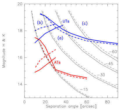
Figure 7: Accessibility to faint stars in terms of magnitude and separation angle in the $H$ and $K$ bands (respectively dashed and full lines). The 3 domains of Fig. 6 for SPR are recalled here with thick lines for ATs and UTs observations. The upper right limit of the domain (c) is omitted for clarity. The thin curves indicate that there are 3 stars in average within the half cone of the corresponding separation and brighter than the corresponding magnitude. These curves are labelled with the galactic latitude of the target direction.

The newly identified domain (a) for SPR with short exposure is useful only if there are stars satisfying the magnitude and separation constraints shown in Fig. 6. We first consider phase-referencing for the astrometric search of exoplanets orbiting bright stars, i.e. bright enough for main delay tracking. We would like to measure the angular separation between a main target and reference stars in its surrounding. As randomly choosen stars can turn out to be binaries, we take a conservative value of 3 reference stars (in average) within the useful solid angle. Reference stars for differential astrometry will most often be faint objects, so that we must rely on star count models for their distribution with galactic coordinates. Our results are based on the Besançon model on stellar populations in our Galaxy (Reylé & Robin (2001)). The half cone angle with 3 stars (in average) brighter than a given magnitude $m$ is taken as $[N(m)]^{-1/2}$, where $N(m)$ is the cumulative density of stars brighter than $m$. Results shown in Fig. 7 are for a region of the sky suited for phase measurements, with a nearly zenith transit at Paranal. Its galactic longitude is $-15$ degrees, and the latitude range is from $-15$ to $-60$ degrees. Whatever the target direction, 3 stars are likely to be found with UTs and SPR with short exposure (domain (a)). At a galactic latitude of $-60$ degrees, the separation angle reaches 1 arcmin and faint star magnitude 17.5. Long exposure SPR with fainter and closer stars is also possible, say 19.5 magnitude and about 42”, but in a regime where the useful photon flux from the star is one tenth the photon flux from the sky background in the $K$ band. Closer to the galactic plane, SPR with short exposure is much easier due to the greater star density.

Figure 8: Probability of finding a guide star for main delay tracking in the vicinity of any target direction with galactic latitudes 15, 30, 45 and 60 degrees. The guide star has to be brighter than K=11.0 (top), 13.0 (middle) or 14.0 (bottom).

A different estimate has to be performed for phase-referenced imaging of a faint object. What is needed is a bright star in its surrounding for main delay tracking. The bright (or guide) star lies in the magnitude range of near-IR surveys, and our estimate of sky-coverage is based on the Second Release of the 2MASS survey . The probability of finding at least one star brighter than $K_{lim}$ has been estimated in terms of the size of the solid angle for phase-referencing, at different galactic latitudes (Fig. 8). Results on positive and negative galactic latitudes have been averaged, and the magnitude limit for the guide star is $K_{lim}$ = 11 (with two ATs), and 13 or 14 (with two UTs). Taking a galactic latitude of 30 degrees as an average sky density, the probability of finding a guide star with 2 ATs ($K_{lim}\leq 11$, within 20”) is about 2%. Significant sky coverage, with a probability of 50%, will be reached only with 2 UTs and improved corrections for the atmospheric turbulence ($K_{lim}\leq 14$ and AO corrections in two different directions, up to 1’ apart).

6 Discussion

The useful angular range for phase-referencing and differential astrometry is not strictly limited, but dependent on the magnitude of the faint object (Fig. 7). Then, the ‘isopistonic’ angle that has been defined in the literature is too restrictive. In our analysis, there exists a specific angle given by the ‘triple-point’ in Fig. 6, where the 2-sample phase rms equals 1 radian at a local minimum. The separation angle and the magnitude of the faint object at this triple-point depend both on the interferometer sentivity and on the site turbulence. It characterizes a whole system (atmosphere + telescope + instrument). An interesting finding of our calculation is that the triple-point is located at about (20”, 16) for ATs and (30”, 18.3) for UTs with similar instruments. This makes a very significant difference in sky coverage, differential astrometry with ATs being limited to rather dense stellar fields (Fig. 7).

Short exposure measurements of differential phase fluctuations integrate various contributions: differential piston, sky background variations, interferometer/instrument instabilities …Short term measurements can then be edited, filtered and weighted before being averaged to properly extract source structure and relative position information. The similar sensitivities and star counts obtained in the $H$ and $K$ bands (Fig. 7) must be stressed, as dual-band observations allow more robust procedures than single band near the magnitude limit.

In our analysis, Adaptive Optics has not been addressed, whereas wavefront corrections are needed in the two sources direction, at least with large telescopes. Tomographic sensing of the atmospheric turbulence with the observation of several guide stars has been proposed for wavefront corrections on a whole telescope FOV (Tallon & Foy (1990)). The technique is known as Multi Conjugate Adaptive Optics (MCAO). Although mainly concerned with improved Strehl Ratio, MCAO is supposed to correct for atmospheric turbulence in a whole volume, and hence to correct for differential pathlength fluctuations on any entrance pupil. Differential interferometric piston ($\Delta$OPD) should be significantly reduced, allowing for long term averaging in faint object imaging on a whole telescope FOV. However, it is difficult to know how much $\Delta$OPD would be reduced since corrugations with large scale lengths, about the pupil size, are less efficiently corrected than shorter scale lengths.

Sky coverage with natural guide stars was thought to be a main problem for AO and not too large telescopes. An efficient technique for MCAO has been proposed recently (Ragazzoni et al. (2002)). It is layer-oriented, with multiple Field of View: a large annular FOV is used for sensing low altitude turbulence, whereas a narrower FOV (about 2’) in the telescope axis is used for sensing high altitude turbulence. Sky coverage exceeding 50% should be reached with 8m telescopes and a wavefront sensor in the R band. Such a sky coverage is quite consistent with our estimate on spatial phase-referencing in dual-field optical interferometry in the near-IR. It makes faint source imaging with VLTI/UT a very promissing next development step.

With the AO system being presently implemented at the Coudé focus of UTs (MACAO), faint source imaging will be restricted to the isoplanatic patch of guide stars. It may reach the telescope FOV of 2 arcmin when turbulence in the upper layers of the atmosphere is particularly weak. For bright enough targets, our analysis shows that $\Delta$OPD will be measured and tracked well beyond the isoplanatic angle.