A Unified Treatment of the Gamma-Ray Burst 021211 and Its Afterglow Emissions

Abstract

The Gamma-Ray Burst (GRB) 021211 detected by the High Energy Transient Explorer (HETE) II had a simple light-curve in the x-ray and gamma-ray energy bands containing one peak and little temporal fluctuation other than the expected Poisson variation. Such a burst offers the best chance for a unified understanding of the gamma-ray burst and afterglow emissions. We provide a detailed modeling of the observed radiation from GRB 021211 both during the burst and the afterglow phase. The consistency between early optical emission (prior to 11 minutes), which presumably comes from reverse shock heating of the ejecta, and late afterglow emission from forward shock (later than 11 minutes) requires the energy density in the magnetic field in the ejecta, expressed as fraction of the equipartition value or $\epsilon_{B}$, to be larger than the forward shock at 11 minutes by a factor of about 10³. We find that the only consistent model for the gamma-ray emission in GRB 021211 is the synchrotron radiation in the forward shock; to explain the peak flux during the GRB requires $\epsilon_{B}$ in forward shock at deceleration to be larger than the value at 11 minutes by a factor of about 10².

These results suggest that the magnetic field in the reverse shock and early forward shock is most likely frozen-in-field from the explosion, and therefore a large fraction of the energy in the explosion was initially stored in magnetic field. We can rule out the possibility that the ejecta from the burst for GRB 021211 contained more than 10 electron-positron pairs per proton.

1 Introduction

Considerable progress has been made in the last few years toward an understanding of the nature of the enigmatic Gamma-Ray Bursts. Much of this progress has resulted from the observation and analysis of afterglow emission - the radiation we receive after the high energy gamma-ray photons ceases - which is firmly established to be synchrotron radiation from a relativistic, external shock (e.g. Wijers, Rees, and Mészáros 1997). The nature of the explosion and the process that generates gamma-ray photons continue to be debated, although it is widely accepted that these explosions involve a stellar mass object. The detection of narrow emission lines (e.g. Greiner et al. 2003) and the emergence of a spectrum similar to that of SN 1998bw (Matheson et al. 2003) in the afterglow of GRB 030329 indicate that at least some GRBs are produced when a massive star undergoes collapse at the end of its nuclear burning life.

Further progress toward understanding the GRB explosion requires afterglow observations at times closer to the burst and a simultaneous modeling of both the afterglow and gamma-ray emissions. In this way, one can explore distance scales of $\sim 10^{16}$cm from the center of explosion, i.e. an order of magnitude smaller than that probed by afterglow emissions at half a day or later. Such a treatment is more likely to succeed in those cases where the prompt (burst) emission arises from the same region as the delayed (afterglow) emission, i.e. from an external shock. The simple FRED-like (fast rise, exponential decay) light-curves seen in about 10% of bursts represents the type expected from an external shock (Mészáros & Rees 1993), while short variability timescale bursts with complicated light curves are usually attributed to internal shocks in an unsteady outflow (Rees & Mészáros 1994; see Piran 1999 & Mészáros 2002 for recent reviews).

This paper is an attempt to explain with the same process – synchrotron and inverse Compton emission from an external shock – the burst and afterglow emission of GRB 021211 detected by the HETE II (Crew et al. 2003), a burst which had a simple, FRED-like morphology and whose afterglow has been followed starting from 60 seconds until 10 days after the burst. In §2 we summarize the observations of GRB/afterglow 021211. In §3–§5 we present the formalism for calculating the synchrotron and inverse Compton emissions from both the forward and reverse shocks, and in §6 and §6.2 we assess the ability of the synchrotron, self-Compton model with a uniform and an $r^{-2}$ stratified medium to accommodate the properties of the GRB 021211 and its afterglow.

2 Summary of Observations for GRB 021211

At a redshift $z=1.0$, GRB 021211 had a duration of $\mathrel{\hbox to0.0pt{\raise 2.20013pt\hbox{$>$}\hss}{\lower 2.20013pt\hbox{$\sim$}}}2.3$s in the 30-400 kev energy band and a fluence of $\sim 2\times 10^{-6}$ erg (Crew et al. 2003); the duration in the 10-25 kev band was $\sim 4$s. If both the burst and the afterglow for GRB 021211 arise from some combination of reverse and forward external shocks, then the deceleration time $t_{d}$ is close to the time when the GRB light-curve peaks in 30-400 kev band, i.e. about 2 seconds. The average flux during the first 2.3s was 4 mJy in the 7-30 kev band, 3 mJy in the 50-100 kev band, and 0.5 mJy in at 100-300 kev, while the peak of the $\nu F_{\nu}$ spectrum was at $47^{+9}_{-7}$ kev. The isotropic equivalent of the energy released in the 10-400 kev emission is $\sim 10^{52}$ erg.

At 90s after the burst, the R-band magnitude of the afterglow 021211 was 14.06 (Wozniak et al. 2002), corresponding to a flux of 7.2 mJy. The optical flux decayed as $t^{-1.82\pm 0.02}$ for the first 10 minutes, after which it flattened to a $t^{-0.82\pm 0.11}$ fall-off (Li et al. 2003), reaching magnitude 25 at 7 days (Fruchter et al. 2002). The steeper decay seen during the first 10.8 minutes suggests that the optical emission is dominated by the reverse shock energizing the GRB ejecta, while the shallower, later time decay is attributed to the forward shock that sweeps-up the ambient medium. The R-band flux at 11 minutes, when the two contributions are equal, is 0.39 mJy, therefore the forward shock optical flux at 11 minutes is 0.19 mJy. Fox et al. (2003) report a 3-$\sigma$ upper limit of 110 $\mu$Jy on the radio (8.5 GHz) flux at 0.1 days, and an upper limit of 35 $\mu$Jy during 9–25 days.

Finally, Milagro has reported an upper limit of $4\times 10^{-6}$erg cm^-2 on the 0.2-20 Tev fluence over the burst duration reported by the HETE WXM (McEnery et al. 2002).

3 Shock dynamics & deceleration time

Consider an explosion where the isotropic equivalent of energy release is ${\cal E}$ and the initial Lorentz factor (LF) of cold baryonic material carrying this energy is $\Gamma_{0}$. Before the ejecta are significantly decelerated, the thermal LF $\gamma_{p,f}$ of the protons in the forward shock (FS), equal to the the bulk LF $\Gamma_{d}$ of the swept-up medium, is (e.g. Piran 1999)

$$\gamma_{p,f}=\Gamma_{d}\approx(\Gamma_{0}/2)^{1/2}(n_{ej}/n)^{1/4},$$ (1)

where $n_{ej}$ is the comoving particle density of the ejecta, and $n=(A/m_{p})r^{-s}$ is the radial profile of the external particle density ($s=0$ for a homogeneous medium, $s=2$ for a pre-ejected wind). The above result holds for $n_{ej}/n\mathrel{\hbox to0.0pt{\raise 2.20013pt\hbox{$<$}\hss}{\lower 2.20013pt\hbox{$\sim$}}}\Gamma_{0}^{2}$, otherwise $\gamma_{p,f}\approx\Gamma_{0}$.

Taking into account that the laboratory frame energy per FS-heated proton is $\Gamma_{d}\gamma_{p,f}=\gamma_{p,f}^{2}$, the deceleration radius $R_{d}$ at which the energy of the swept-up medium is half the initial energy of the ejecta is

$${4\pi\over 3-s}R_{d}^{3-s}Ac^{2}\Gamma_{0}\left({n_{ej}\over n}\right)^{1/2}={\cal E}.$$ (2)

As long as the distribution of LF of the ejecta is not too narrow, and the duration of the central explosion is less than $R/(c\Gamma_{0}^{2})$, the comoving width of the material ejected in the explosion is proportional to $R/\Gamma_{0}$. Let us parametrize the comoving thickness of the ejecta as $\eta R/\Gamma_{0}$. Therefore, the comoving density of the ejecta is

$$n_{ej}=\frac{{\cal E}}{4\pi R^{3}\eta m_{p}c^{2}},$$ (3)

which substituted in equation (2) leads to

$$R_{d}=c\left[{(3-s)^{2}\eta{\cal E}\over 4\pi Ac^{2}\Gamma_{0}^{2}}\right]^{1\over 3-s}.$$ (4)

This result is identical to that obtained for the Blandford-McKee self-similar solution extrapolated back to $R_{d}$ if we set $\eta=17/18$ for $s=0$ and $\eta=9/2$ for $s=2$.

From equations (3) and (4), the comoving density of the ejecta at $R_{d}$ is

$${n_{ej}\over n}(R_{d})={\Gamma_{0}^{2}\over(3-s)^{2}\eta^{2}},$$ (5)

for $\eta\mathrel{\hbox to0.0pt{\raise 2.20013pt\hbox{$>$}\hss}{\lower 2.20013pt\hbox{$\sim$}}}1$. Substituting this into equation (1), the LF of the shocked ISM at $R_{d}$ is

$$\Gamma_{d}={\Gamma_{0}\over\left[2(3-s)\eta\right]^{1/2}}.$$ (6)

From equations (4) and (6), the observer-frame deceleration timescale is

$$t_{d}=(1+z)f_{\eta}{R_{d}\over c\Gamma_{d}^{2}}={(1+z)f_{\eta}\over c\,\Gamma_{0}^{2}}\left[{(3-s)^{5-s}\eta^{4-s}{\cal E}\over 4\pi Ac^{2}\Gamma_{0}^{2}}\right]^{1\over 3-s},$$ (7)

where $f_{\eta}$ is a correction factor that takes into account the difference between the arrival time $(1+z)R_{d}/(2c\Gamma_{d}^{2})$ of photons emitted from the contact discontinuity and that from where most of the GRB emission arises. The lab frame speed of the reverse shock relative to the back-end of the shell, shown in figure 1, is $V_{rs,lab}/c\approx 1.4(3-s)\eta/\Gamma_{0}^{2}$. Thus, the time it takes for the RS to cross the shell (in lab frame) is, $\eta R_{d}/(\Gamma_{0}^{2}V_{rs,lab})\approx[1.4(3-s)]^{-1}R_{d}/c$. And so the RS crossing time is same as the deceleration time to within a factor of order unity.

For $t>t_{d}$ the LF decreases as

$$\Gamma(t)=\Gamma_{d}\left({t\over t_{d}}\right)^{-{3-s\over 8-2s}}.$$ (8)

4 Forward Shock

The comoving density behind the forward shock (FS) is, $\rho=4\rho_{0}\Gamma$, and the thermal energy density is $u=4\rho_{0}c^{2}\Gamma^{2}$; where $\rho_{0}=Ar^{-2}$ is the density of the medium just ahead of the shock, and $\gamma$ is the bulk LF of shocked fluid given by equation (8). A fraction $\epsilon_{e}$ of the thermal energy of the shock-heated circumburst medium is taken up by electrons. Electrons with thermal LF greater than $\gamma_{i}$ are assumed to have a powerlaw distribution with index $p$, i.e. $dN_{e}/d\gamma\propto\gamma^{-p}$ for $\gamma>\gamma_{i}$, where $\gamma_{i}=\epsilon^{\prime}_{e}(m_{p}/m_{e})\gamma_{p}$, is the minimum thermal LF of electrons; $\epsilon_{e}^{\prime}=[(p-2)/(p-1)]\epsilon_{e}$ for $p>2$ and $\gamma_{p}$ is the proton thermal LF. The energy density in magnetic field is assumed to be $\epsilon_{B_{f}}u$, and therefore the magnetic field is $B=4\Gamma c(2\pi\epsilon_{B_{f}}Ar^{-2})^{1/2}$.

The FS synchrotron injection frequency, $\nu_{if}$ and the flux at the peak of the $F_{\nu}$ spectrum, are

$$\nu_{if}(t)={qB\gamma_{i}^{2}\Gamma\over 2\pi m_{e}c(1+z)}={4q\epsilon_{e}^{\prime}{{}^{2}}\epsilon_{B_{f}}^{1\over 2}m_{p}^{2}A^{1\over 2}\Gamma_{d}^{4-s}\over\sqrt{2\pi}\,m_{e}^{3}(1+z)}\left[{4(4-s)ct_{d}\over 1+z}\right]^{-s/2}\left({t\over t_{d}}\right)^{-3/2},$$ (9)

$$f_{\nu_{p},f}(t)={N_{e}\epsilon^{\prime}_{\nu^{\prime}_{p}}\Gamma\over d_{L}^{{}^{\prime 2}}}={4(6\pi)^{1/2}q^{3}A^{3\over 2}\epsilon_{B_{f}}^{1\over 2}\Gamma_{d}^{8-3s}\over m_{p}m_{e}c(3-s){d_{L}^{\prime}}^{2}}\left[{4(4-s)ct_{d}\over 1+z}\right]^{3(2-s)\over 2}\left({t\over t_{d}}\right)^{-{s\over 8-2s}},$$ (10)

where $q$ & $m_{e}$ are electron charge and mass, $m_{p}$ is proton mass, and $d_{L}^{\prime}=D_{L}/\sqrt{1+z}$, $D_{L}$ being the luminosity distance, $N_{e}=AR^{3-s}/(3-s)$ is the number of electrons per unit solid angle behind the shock, and $\epsilon^{\prime}_{\nu^{\prime}_{p}}=3^{1/2}q^{3}B/m_{e}c^{2}$ is power per unit frequency per electron, in comoving frame, at the peak of the synchrotron spectrum.

The synchrotron injection frequency for the cases of $s=0$ & 2 are written out explicitly for ease of application later on

$$\nu_{if}(t)={\epsilon_{e}^{\prime}}^{2}\epsilon_{B_{f_{-4}}}^{1\over 2}(t/t_{d})^{-{3\over 2}}\times\Biggl{\{}{\parbox{219.08612pt}{\@@eqnarray 3.7\times 10^{18}n_{0}^{1/2}\Gamma_{d_{2}}^{4}(1+z)^{-1}\;{\rm Hz}\quad\quad\quad{\rm s=0}\\ 1.7\times 10^{21}A_{*}^{1/2}\Gamma_{d_{2}}^{2}t_{d}^{-1}\;{\rm Hz}\;\quad\quad\quad\quad\quad{\rm s=2}\cr}}\Biggr{.}$$

where $A_{*}=A/5$x$10^{11}$ g cm^-1, and an integer subscript $n$ on a variable $X$, $X_{n}$, means $X/10^{n}$. The flux at the peak of the synchrotron spectrum for $s=0$ & 2 is

$$f_{\nu_{p},f}(t)=\epsilon_{B_{f_{-4}}}^{1\over 2}\Gamma_{d_{2}}^{2}\times\Biggl{\{}{\parbox{187.78836pt}{ \@@eqnarray 5.5\times 10^{-7}n_{0}^{3/2}\Gamma_{d_{2}}^{6}t_{d}^{3}\;{\rm mJy}\quad\quad\quad{\rm s=0}\\ 1.2\times 10^{3}A_{*}^{3/2}(t/t_{d})^{-1/2}\;{\rm mJy}\;\quad{\rm s=2}\cr }}\Biggr{.}$$

In the derivation of the above equation we have set $z=1$ which corresponds to the redshift of GRB 021211.

The FS synchrotron self-absorption frequency ($\nu_{Af}$), obtained by equating the intensity at $\nu_{Af}$ to $2m_{e}\gamma_{if}\nu_{Af}^{2}$, is given by

$$\nu_{Af}^{2}\left({\nu_{if}\over\nu_{Af}}\right)^{\alpha}={(6\pi\epsilon_{B})^{1/2}q^{3}A^{3\over 2}\Gamma_{d}^{4-3s}(4t_{d})^{(2-3s)/2}\over 8(3-s)m_{e}m_{p}^{2}\epsilon^{\prime}_{e}(1+z)^{(6-3s)/2}c^{3s/2}}\left({t\over t_{d}}\right)^{-{s+4\over 8-2s}},$$ (13)

where $\alpha$ depends on the relative location of $\nu_{Af}$ with respect with $\nu_{if}$ and the cooling frequency $\nu_{cf}$; for $\nu_{cf}>\nu_{if}>\nu_{Af}$, $\alpha=1/3$, and $\alpha=p/2$ if $\nu_{if}<\nu_{Af}<\nu_{cf}$.

4.1 Application to GRB 021211 late time optical observation

We make use of the optical R-band flux at late time, $t\geq 11$min, to provide constraints on the density, $\epsilon_{Bf}$ & $\Gamma_{d}$ for $s=0$ and $s=2$ cases separately.

4.1.1 Parameters for a uniform ISM model

Using equation (7) the bulk LF at deceleration time, for $s=0$, is found to be

$$\Gamma_{d_{2}}=3.8\left({{\cal E}_{52}\over n_{0}}\right)^{1/8}\left[{f_{\eta}(1+z)\over t_{d}}\right]^{3/8},$$ (14)

where $n_{0}$ is density of the uniform ISM, $f_{\eta}=\max\{1,2\sqrt{\eta}/3\}$ (see footnote 2) and an integer subscript on a variable $X_{n}$ means $X/10^{n}$.

The observed R-band flux at 11 min for GRB 021211 is 0.4 mJy. According to the fit presented in Li et al. (2003) the contributions from the reverse and forward shocks to the observed R-band flux are equal at this time. Therefore, the FS peak flux at 11 min is greater than 0.2 mJy; we will consider the peak flux to be $0.2\,A_{f}$ mJy, with $A_{f}>1$. It should be noted that for $s=0$ the peak flux is time independent. Substituting this into equation (4), and making use of equation (14) to eliminate $\Gamma_{d}$ we find

$$n_{0}^{1\over 2}{\cal E}_{52}\epsilon_{B_{f_{-4}}}^{1\over 2}=A_{f}f_{\eta}^{-3}.$$ (15)

The R-band lightcurve is observed to be monotonically declining from the earliest time (90s), and from 11 min to 10 days the decline is a simple powerlaw with index $0.82\pm 0.11$. Thus, the frequency of the peak of the spectrum at 11 min is expected to be less than the R-band frequency of 4.7x$10^{14}$ Hz or 1.95 ev. Let us assume that the peak frequency at 11 min is a factor $A_{\nu}$ smaller than the R-band frequency. Substituting this into equation (4) and making use of equation (14) we find

$${\cal E}_{52}^{1/2}\epsilon_{B_{f_{-4}}}^{1/2}\epsilon_{e}^{\prime}{{}^{2}}f_{\eta}^{3/2}=8\times 10^{-3}A_{\nu}^{-1}\quad{\rm or}\quad\epsilon_{B_{f}}(t=11min)=6.4\times 10^{-9}A_{\nu}^{-2}{\cal E}_{52}^{-1}\epsilon_{e}^{\prime}{{}^{-4}}f_{\eta}^{-3}.$$ (16)

The synchrotron peak frequency as a function of time is given by

$$\nu_{if}=37.3\,t^{-3/2}A_{\nu}^{-1}\;{\rm kev},$$ (17)

Combining equations (14), (15) and (16) we find

$$\Gamma_{d_{2}}^{2}\approx 2.2\,(A_{\nu}A_{f})^{-1/2}f_{\eta}^{3/2}{\cal E}_{52}^{1/2}\epsilon_{e}^{\prime-1}t_{d}^{-3/4}.$$ (18)

Substituting this back into equation (14) we obtain

$$n_{0}=1.5\times 10^{4}\,(A_{\nu}A_{f})^{2}{\cal E}_{52}^{-1}f_{\eta}^{-3}\epsilon_{e}^{\prime}{{}^{4}}\;\;{\rm cm}^{-3}.$$ (19)

Note that $A_{f}$ and $A_{\nu}$ are related by $A_{f}=A_{\nu}^{(p-1)/2}$, if the cooling frequency ($\nu_{c}$) is above the R-band at 11 min, and $A_{f}=A_{\nu}^{p/2}$ if $\nu_{c}$ is below the R-band. For ${\cal E}_{52}=1$, $\epsilon_{e}=0.5$, $A_{\nu}=4$ & $p=2.2$ we find $n_{0}=61$ cm^-3, $\Gamma_{d}=250$, and $\epsilon_{B}=8\times 10^{-6}$.

4.1.2 Parameters for $s=2$ model from late time Optical data

The deceleration time for $s=2$ is given by (see eq. 7)

$$t_{d}=0.08(1+z){{\cal E}_{52}f_{\eta}\over A_{*}\Gamma_{d_{2}}^{4}}\quad{\rm s},$$ (20)

where $A_{*}=A/5$x$10^{11}$g cm^-1 & $f_{\eta}=\max(1,\sqrt{2\eta}/3)$. Since the peak flux at 11 min is 0.2 $A_{f}$ mJy, we find using equation (4), the FS peak flux at an earlier time to be

$$f_{\nu_{p},f}=5.4\,A_{f}t^{-1/2}\quad{\rm mJy},$$ (21)

and

$$A_{*}^{3/2}\epsilon_{B_{f_{-4}}}^{1/2}t_{d}^{1/2}\Gamma_{d_{2}}^{2}=4.5\times 10^{-3}A_{f}$$ (22)

Taking the synchrotron peak frequency at 11 min to be 4.7x10${}^{14}A_{\nu}^{-1}$ Hz, and substituting this into equation (4) we obtain for $s=2$

$$A_{*}^{1/2}\epsilon_{e}^{\prime}{{}^{2}}\epsilon_{B_{f_{-4}}}^{1/2}\Gamma_{d_{2}}^{2}t_{d}^{1/2}=5\times 10^{-3}A_{\nu}^{-1},$$ (23)

and the time evolution of $\nu_{if}$ is same as in equation (17).

From equations (22) and (23) we obtain

$$A_{*}=0.9\,\epsilon_{e}^{\prime}{{}^{2}}(A_{\nu}A_{f}),$$ (24)

which when substituted into equation (20) gives the LF at deceleration

$$\Gamma_{d_{2}}=0.7\,{\cal E}_{52}^{1/4}t_{d}^{-1/4}f_{\eta}^{1/4}\epsilon_{e}^{\prime-1/2}(A_{\nu}A_{f})^{-1/4}.$$ (25)

Combining equations (23), (24) and (25) we obtain

$$\epsilon_{B_{f}}(t=11min)=1.7\times 10^{-8}A_{\nu}^{-2}f_{\eta}^{-1}{\cal E}_{52}^{-1}\epsilon_{e}^{\prime}{{}^{-4}}.$$ (26)

We see from these equations that for $s=2$, $A_{\nu}$ can be as large as 10-20, and yet give acceptable values for various parameters.

5 Reverse Shock

The emission from reverse shock (RS) in gamma-ray bursts is discussed by a number of authors e.g. Panaitescu & Mészáros (1998), Sari & Piran (1999), Kobayashi (2000), Piran (2000). A particularly important parameter that determines the behavior of RS is the thickness of the shell of material or ejecta that carries the relativistic energy of the explosion. We have parametrized the ejecta thickness as $\eta R/\Gamma_{0}^{2}$ in lab frame; for a shell whose thickness is dominated by expansion at deceleration radius we expect $\eta\sim 1$, otherwise the thickness is determined by the duration of the central engine, and $\eta$ could be much larger than unity at $t_{d}$. We calculate RS emission for a range of $\eta$ between 0.5 and 10. Fortunately the main conclusions of this work for GRB 021211 remain unchanged even for a larger range of $\eta$.

At the deceleration radius $R_{d}$, the ratio of the thermal energy of protons in the reverse shock (RS) region, $\gamma_{p,r}$, to that in the FS, $\gamma_{p,f}$, is (see fig. 1)

$${\gamma_{p,r}\over\gamma_{p,f}}\approx{1\over 4\Gamma_{0}}\left({n_{ej}\over\Gamma_{0}^{2}n}\right)^{-0.7}\approx{\left[(3-s)\eta\right]^{1.4}\over 4\Gamma_{0}}={\left[(3-s)\eta\right]^{0.9}\over\sqrt{32}\,\Gamma_{d}}.$$ (27)

The first part in the above equation is valid only for $0.01\mathrel{\hbox to0.0pt{\raise 2.20013pt\hbox{$<$}\hss}{\lower 2.20013pt\hbox{$\sim$}}}n_{ej}/\Gamma_{0}^{2}n\mathrel{\hbox to0.0pt{\raise 2.20013pt\hbox{$<$}\hss}{\lower 2.20013pt\hbox{$\sim$}}}100$; for $n_{ej}/\Gamma_{0}^{2}n\ll 0.01$, it can be shown that $\gamma_{p,r}/\gamma_{p,f}\simeq(n_{ej}/n)^{-0.5}$. In deriving the second part of this equation we made use of (5) for the density of the ejecta at $R_{d}$ — $n_{ej}(R_{d})$. It should be noted that the thermal energy per proton in RS is $\sim m_{p}c^{2}\eta^{0.9}/32^{1/2}$, and so protons are not heated to a relativistic temperature in the reverse shock.

The pressure continuity across the contact discontinuity surface, which separates forward and reverse shocks, implies that the magnetic field strength in RS and FS are equal, provided that $\epsilon_{B}$ is the same behind both shocks. However, one might expect $\epsilon_{B}$ in the RS ($\epsilon_{Br}$) to be different from the value in FS ($\epsilon_{Bf}$). Then the synchrotron peak frequency in the RS is

$$\nu_{ir}(t_{d})=\nu_{if}(t_{d})\left(\frac{\epsilon_{Br}}{\epsilon_{Bf}}\right)^{1/2}\left({\gamma_{p,r}\over\gamma_{p,f}}\right)^{2}_{t_{d}}=\nu_{if}(t_{d}){\left[(3-s)\eta\right]^{1.8}\over 32\Gamma_{d}^{2}}\left(\frac{\epsilon_{Br}}{\epsilon_{Bf}}\right)^{1/2}.$$ (28)

This can be written out explicitly as follows

$$\nu_{ir}(t_{d})={qm_{p}^{2}\epsilon_{Br}^{1\over 2}{\epsilon^{\prime}_{e}}^{2}A^{1\over 2}R_{d}^{-{s\over 2}}\Gamma_{d}^{2}[(3-s)\eta]^{1.8}\over(128\pi)^{1/2}(1+z)m_{e}^{3}},$$ (29)

or

$$\nu_{ir}(t_{d})=\epsilon_{B_{r_{-4}}}^{1/2}\epsilon_{e}^{\prime}{{}^{3}}(A_{\nu}A_{f})^{1/2}\eta^{1.8}\times\Biggl{\{}{\parbox{142.26378pt}{\@@eqnarray 1.1\times 10^{16}t_{d}^{-3/4}\;{\rm Hz}\quad\quad\quad\quad{\rm s=0}\\ 5.1\times 10^{15}t_{d}^{-1}\quad{\rm Hz}\quad\quad\quad\quad{\rm s=2}\cr }}\Biggl{.}$$

In deriving this last equation we made use of equations (18), (19), (24) & (25) for ISM density and LF at deceleration.

Since the FS and RS region are moving at same LF, at deceleration, the RS peak synchrotron flux is equal to the FS peak flux times the ratio of number of electrons in the ejecta to the swept-up electrons in the surrounding medium up to $R_{s}$; this ratio is equal to $\Gamma_{0}/(3-s)\eta=[2/(3-s)\eta]^{1/2}\Gamma_{d}$. Thus, the RS peak flux is

$$f_{\nu_{p},r}(t_{d})=f_{\nu_{p},f}(t_{d})\left[{2(\epsilon_{Br}/\epsilon_{Bf})\over(3-s)\eta}\right]^{1/2}\Gamma_{d},$$ (31)

or

$$f_{\nu_{p},r}(t_{d})={(3\epsilon_{Br}A)^{1\over 2}q^{3}{\cal E}(1+z)^{s\over 2}\over m_{e}m_{p}c^{3}d_{L}^{\prime 2}\Gamma_{d}^{s-1}(4ct_{d})^{s\over 2}[\pi(3-s)\eta]^{1\over 2}}.$$ (32)

Using equations (18), (19), (24) & (25) this equation reduces to

$$f_{\nu_{p},r}(t_{d})=\epsilon_{B_{r_{-4}}}^{1/2}\epsilon_{e}^{\prime}{{}^{3/2}}(A_{\nu}A_{f})^{3/4}{\cal E}_{52}^{3/4}\eta^{-1/2}\times\Biggl{\{}{\parbox{187.78836pt}{ \@@eqnarray 2.9\times 10^{3}t_{d}^{-3/8}\quad{\rm mJy}\quad\quad\quad\quad{\rm s=0}\\ 3.8\times 10^{4}t_{d}^{-3/4}\quad{\rm mJy}\quad\quad\quad\quad{\rm s=2}\cr }}\Biggr{.}$$

The RS synchrotron self-absorption frequency is

$$\nu_{Ar}^{2}(t_{d})\left({\nu_{ir}\over\nu_{Ar}}\right)^{\alpha}={q^{3}E\left[6\pi\epsilon_{B}A(1+z)^{s}\right]^{1/2}\over 8\pi m_{e}m_{p}^{2}c^{3}\epsilon_{e}^{\prime}[(3-s)\eta]^{1.4}(4ct_{d})^{s+4\over 2}\Gamma_{d}^{s+2}},$$ (34)

where $\alpha=1/3$ if $\nu_{ir}>\nu_{Ar}$, and $p/2$ otherwise. Using equations (18), (19), (24) & (25) this can be rewritten as

$$\nu_{Ar}(t_{d})\left({\nu_{ir}\over\nu_{Ar}}\right)^{\alpha/2}=\epsilon_{B_{r_{-4}}}^{1/4}\epsilon_{e}^{\prime}(A_{\nu}A_{f})^{3/4}\eta^{-0.7}\times\Biggl{\{}{\parbox{170.71652pt}{\@@eqnarray 5.5\times 10^{13}t_{d}^{-5/8}\;{\rm Hz}\;\quad\quad\quad\quad{\rm s=0}\\ 1.1\times 10^{15}t_{d}^{-1}\quad{\rm Hz}\;\quad\quad\quad\quad{\rm s=2}\cr }}\Biggr{.}$$

5.1 Time dependence of radiation from reverse shock

The time dependence for $\nu_{ir}$ & $f_{\nu_{p},r}$ is determined by the evolution of magnetic field and electron thermal energy in the reverse shock. Electrons in the ejecta cease to be heated after the passage of the RS, and their energy decreases with time as a result of adiabatic expansion. If electrons continue to exchange energy with protons, and the fraction of thermal energy in electrons, $\epsilon_{e}$, is time independent, then electron thermal LF decreases as

$$\gamma_{e}\propto(R^{2}\delta R)^{-{2-\epsilon_{e}\over 3}}\propto t^{-{2(2-\epsilon_{e})\over 3(4-s)}},$$ (36)

where $\delta R$ is the comoving shell thickness which is a weak function of time for sub- or mildly-relativistic RS, and $R$, the radius of the ejecta, increases with time as $t^{1/(4-s)}$; $\epsilon_{e}=1$ if electrons and protons are decoupled.

The magnetic field, frozen in the ejecta, decreases as $B^{\prime}\propto(R\delta R)^{-1}\propto t^{-1/(4-s)}$ if the field is transverse; a longitudinal field decreases as $t^{-2/(4-s)}$, therefore any non-zero transverse field will become the dominant component at large distances.

The synchrotron injection frequency and the peak flux decrease as

$$\nu_{ir}\propto B^{\prime}\gamma_{e}^{2}\Gamma\propto t^{-{31-3s-8\epsilon_{e}\over 6(4-s)}},\quad{\rm and}\quad f_{\nu_{p},r}\propto N_{e}\,B^{\prime}\Gamma\propto N_{e}t^{-{5-s\over 2(4-s)}},$$ (37)

where $N_{e}$ is the total number of “radiating” electrons in the ejecta.

The cooling frequency decreases at the same rate as $\nu_{ir}$; the decline is faster if radiative losses dominate over adiabatic losses. The number of electrons radiating in an observer band might have a non-trivial time independent if the magnetic field is not constant across the ejecta – electrons in a region of higher magnetic field will lose energy at a higher rate and their radiation drops below the observed band sooner than electrons in lower magnetic field region. This together with uncertainty with the evolution of $\gamma_{e}$ – which depends upon coupling between electrons & protons – and the unknown energy density & LF structure of the ejecta, makes it difficult to calculate with confidence the power-law decay index for flux from reverse shock.

In order to fit the data for GRB 021211 what we do instead is to work backwards from the observed lightcurve slope and determine the decay of synchrotron frequency – which depends on both $B^{\prime}$ and $\gamma_{e}$ and so its time dependence is more uncertain than the peak flux which depends on $B^{\prime}$ alone – that we need to calculate the cooling frequency at 11 minutes after the explosion to make sure that it is above the optical R-band.

Let us consider the time dependence for injection frequency and peak flux to be $t^{-\alpha_{\nu}}$ & $t^{-\alpha_{f}}$ respectively. The flux above the synchrotron peak decays as $t^{-[2\alpha_{f}+(p-1)\alpha_{\nu}]/2}$ ($p$ is electron energy power-law index). The observed decay for GRB 021211 was $t^{-1.8}$, which we use to determine $\alpha_{\nu}$; we assume that $\alpha_{f}$ is as given in equation (37), but allow for a small deviation when fitting the observed data. With $\alpha_{\nu}$ and $\alpha_{f}$ thus determined, we find the time dependence of $B^{\prime}$ & $\gamma_{e}$

$$B^{\prime}\propto t^{-\alpha_{f}+{3-s\over 8-2s}},\quad\quad\gamma_{e}\propto t^{-{\alpha_{\nu}-\alpha_{f}\over 2}},$$ (38)

that we use to calculate absorption and cooling frequencies and flux as a function of time.

5.2 Compton Parameter & Cooling Frequency

The comoving frame timescale for an electron of energy $m_{e}c^{2}\gamma_{e}$ to cool as a result of synchrotron and inverse Compton emission is

$$t^{\prime}_{c}={6\pi m_{e}c\over\sigma_{T}B^{\prime 2}\gamma_{e}(1+Y)}={3m_{e}R_{d}^{s}\over 16\sigma_{T}c\epsilon_{B}\gamma_{e}\Gamma_{d}^{2}A(1+Y)},$$ (39)

where $Y$ is the Compton $Y$ parameter, prime denotes comoving quantity, and the cooling is considered at the deceleration time. At deceleration, when $t^{\prime}_{c}=4t_{d}\Gamma_{d}/(1+z)$, the electron cooling LF, $\gamma_{c}$, defined by the equality of the radiative and dynamical timescales, is

$$\gamma_{c}(t_{d})={3\pi m_{e}c(1+z)\over 2\sigma_{T}B^{\prime 2}t_{d}\Gamma_{d}(1+Y)}={3m_{e}\Gamma_{d}^{2s-3}\over 16\sigma_{T}\epsilon_{B}A(1+z)^{s-1}(4ct_{d})^{1-s}(1+Y)}$$ (40)

Substituting for $A$ and $\Gamma_{d}$ from equations (18), (19), (24) & (25) we obtain

$$\gamma_{c}(t_{d})={{\cal E}_{52}^{1/4}\over\epsilon_{B_{-4}}{\epsilon_{e}^{\prime}}^{5\over 2}(A_{\nu}A_{f})^{5\over 4}(1+Y)}\times\Biggl{\{}{\parbox{113.81102pt}{\@@eqnarray 513\,t_{d}^{1/8}\quad\quad\quad\quad{\rm s=0}\\ 22\,t_{d}^{3/4}\quad\quad\quad\quad{\rm s=2}\cr }}\Biggr{.}$$

The cooling frequency $\nu_{c}$, defined as the synchrotron frequency for electrons with LF $\gamma_{c}$, is

$$\nu_{c}(t_{d})={qB^{\prime}\gamma_{c}^{2}\Gamma_{d}\over 2\pi m_{e}c(1+z)}=6.1\times 10^{-5}{c^{2}(4ct_{d}\Gamma_{d}^{2})^{3s-4\over 2}\over(A\,\epsilon_{B_{-4}})^{3/2}(1+Y)^{2}(1+z)^{(3s-2)/2}}\;\,{\rm Hz},$$ (42)

which can be rewritten by substituting for $A$ and $\Gamma_{d}$

$$\nu_{c}(t_{d})={{\cal E}_{52}^{1/2}\over\epsilon_{B_{-4}}^{3/2}\epsilon_{e}^{\prime 4}(A_{\nu}A_{f})^{2}(1+Y)^{2}}\times\Biggl{\{}{\parbox{187.78836pt}{\@@eqnarray 2\times 10^{15}(1+z)t_{d}^{-1/2}\;\quad{\rm Hz}\;\quad\quad{\rm s=0}\\ 9\times 10^{13}(1+z)^{-2}t_{d}^{1/2}\quad{\rm Hz}\quad\quad{\rm s=2}\cr }}\Biggr{.}$$

The cooling frequencies in the reverse and forward shock regions are calculated from this equation by substituting appropriate values for $\epsilon_{B}$ and $Y$ corresponding to each region. The Compton $Y$ parameter is calculated below.

The electron column density in the ejecta, at the deceleration radius, assuming that the ejecta consists only of protons and electrons, i.e. there are no pairs, is

$$N_{e,r}={{\cal E}\over 4\pi R_{d}^{2}\Gamma_{0}m_{p}c^{2}}={(1+z)^{2}{\cal E}\over 64\pi\sqrt{2(3-s)\eta}\,m_{p}c^{4}t_{d}^{2}\Gamma_{d}^{5}}.$$ (44)

The optical depth of the ejecta to Thomson scattering is

$$\tau_{r}=\sigma_{T}N_{e,r}=1.7\times 10^{-3}{(1+z)^{2}{\cal E}_{52}\over\sqrt{(3-s)\eta}\,t_{d}^{2}\Gamma_{d_{2}}^{5}}.$$ (45)

The Compton parameter $Y=\tau\overline{\gamma_{e}^{2}}$, where $\overline{\gamma_{e}^{2}}$, the mean squared electron LF, for $\nu_{A}<\nu_{i}<\nu_{c}$ & $2<p<3$ is

$$\overline{\gamma_{e}^{2}}={(p-1)\over(p-2)(3-p)}\gamma_{i}^{2}\left({\gamma_{c}\over\gamma_{i}}\right)^{3-p},$$ (46)

and $m_{e}c^{2}\gamma_{i}$ is the minimum thermal energy of shock heated electrons. The Compton parameter in the particular case of $\nu_{A}<\nu_{c}<\nu_{i}$ is given by

$$Y\simeq\left({\epsilon_{e}\over\epsilon_{B}}\right)^{1/2}.$$ (47)

Substituting (5.2) into (46) and making use of equations (27) & (45) we find the Compton $Y$ in the reverse shock region

$$Y(1+Y)^{3-p}={(p-1)m_{p}^{p-1}{\cal E}_{52}^{2-p\over 4}\epsilon_{B_{r_{-4}}}^{p-3}{\epsilon_{e}^{\prime}}^{7p-12\over 2}(A_{\nu}A_{f})^{5(p-2)\over 4}\eta^{0.9p-1.4}\over(p-2)(3-p)m_{e}^{p-1}32^{p-1\over 2}}$$

$$\quad\times\Biggl{\{}{\parbox{150.79968pt}{\@@eqnarray 2.8\times 10^{4}\,191^{-p}t_{d}^{-{p-2\over 8}}\quad\quad{\rm s=0}\\ 6.4\times 10^{2}\,22^{-p}t_{d}^{-3(p-2)\over 4}\quad\quad{\rm s=2}\cr }}\Biggr{.}$$

The Compton $Y$ substituted back into equation (5.2) yields the cooling frequency in RS. A similar calculation gives $\nu_{c}$ in the forward shock.

When $\nu_{A}>\min\{\nu_{c},\nu_{i}\}$, the synchrotron photon flux that is scattered by an electron is diminished by self-absorption and $\nu_{A}$ and $\nu_{c}$ have to be determined by solving a set of coupled equations, as described in Panaitescu & Mészáros (2000). Some of the cases considered for GRB 021211r fall in this more complicated regime, and all of the numerical results presented in this paper are obtained by determining $\nu_{A}$ and $\nu_{c}$ numerically, in a self-consistent manner.

6 A unified modeling for $\gamma$-ray and afterglow data

We apply the results of the last two sections to a systematic analysis of $\gamma$-ray, optical and radio observations for GRB 021211 and determine models that are consistent with all data. We discuss the cases of a uniform density ISM ($s=0$), and a medium carved out by the progenitor’s wind ($s=2$) in two separate subsection.

6.1 A Uniform Density Circumburst Medium (s=0)

In the next subsection we discuss the early optical & radio emissions from the RS. We take up the question of what could have produced the $\gamma$-ray emission in §6.1.2 & radio upper limit in §6.1.3.

6.1.1 Optical and radio emissions from reverse shock

The RS synchrotron injection frequency is a factor of $(\gamma_{p,f}/\gamma_{p,r})^{2}$ smaller compared with the peak frequency of the FS emission as long as $\epsilon_{B}$ is the same in reverse and forward shocks. The synchrotron injection frequency in the RS, otherwise, is expected to be about 2x10${}^{-2}\eta^{1.8}A_{\nu}^{-1}(\epsilon_{Br}/\epsilon_{Bf})^{1/2}$ ev (see eqs. 5 & 16). This suggests that the RS flux in the optical band decreases with time for $t>t_{d}$. The extrapolation of the observed flux of 7.2 mJy at 90s, with a powerlaw decline of $t^{-1.8}$, gives a R-band flux at 5s of 1.3 Jy or 8.5 mag. So, contrary to claims, GRB 021211 was as bright as 990123 close to the deceleration time.

The injection frequency in RS for $s=0$ declines with observer time approximately as $t^{-1}$, and the cooling frequency too declines as $t^{-1}$ or faster. After the passage of the reverse shock, which takes place on the deceleration time scale of a few seconds for GRB021211, electrons are no longer accelerated and there is no emission from RS at a frequency greater than the cooling frequency ($\nu_{cr}$). The R-band flux from GRB 021211 is observed to decline as $t^{-1.8}$ for 11 minutes and then the decline slows down to $t^{-0.8}$. This suggests that the RS emission lasts for at least 11 minutes in the R-band, and therefore $\nu_{cr}$ at deceleration should be $\mathrel{\hbox to0.0pt{\raise 2.20013pt\hbox{$>$}\hss}{\lower 2.20013pt\hbox{$\sim$}}}10^{17}$ Hz.

The inverse Compton parameter and the cooling frequency are determined from equations (5.2) and (5.2). For $p=2.5$ these quantities at the deceleration time are

$$Y(1+Y)^{0.5}=2\times 10^{3}\epsilon_{e}^{\prime 2.75}\epsilon_{B_{r_{-4}}}^{-{1\over 2}}\eta^{0.85}A_{\nu}^{35\over 32}{\cal E}_{52}^{-{1\over 8}}t_{d}^{-{1\over 16}},$$ (49)

and

$$\nu_{cr}=1.5\times 10^{11}{{\cal E}_{52}^{1/2}\over\epsilon_{e}^{\prime 7.7}\epsilon_{B_{r_{-4}}}^{0.83}\eta^{1.1}A_{\nu}^{5}t_{d}^{2/5}}\quad{\rm Hz},$$ (50)

so long as $Y\mathrel{\hbox to0.0pt{\raise 2.20013pt\hbox{$>$}\hss}{\lower 2.20013pt\hbox{$\sim$}}}1$. For $Y\ll 1$ the cooling frequency is obtained by setting $Y=0$ in equation (5.2).

The requirement that $\nu_{cr}(t_{d})>10^{17}$Hz – in order to have non-zero flux in the R-band from RS for $\sim 11$min – provides an upper limit on $\epsilon_{e}^{\prime}$ given below

$$\epsilon_{e}^{\prime}\mathrel{\hbox to0.0pt{\raise 2.20013pt\hbox{$<$}\hss}{\lower 2.20013pt\hbox{$\sim$}}}{0.175\,\,{\cal E}_{52}^{1/15.4}\over\epsilon_{B_{r_{-4}}}^{1/9}A_{\nu}^{2/3}\eta^{1/7}t_{d}^{1/20}}.$$ (51)

Substituting this into (5) & (5) we find the injection frequency and peak flux from the RS

$$\nu_{ir}(t_{d})\mathrel{\hbox to0.0pt{\raise 2.20013pt\hbox{$<$}\hss}{\lower 2.20013pt\hbox{$\sim$}}}6\times 10^{13}\epsilon_{B_{r_{-4}}}^{1/6}{\cal E}_{52}^{1/5.1}A_{\nu}^{-1.1}\eta^{1.37}t_{d}^{-0.9}\quad{\rm Hz},$$ (52)

and

$$f_{\nu_{p},r}(t_{d})\mathrel{\hbox to0.0pt{\raise 2.20013pt\hbox{$<$}\hss}{\lower 2.20013pt\hbox{$\sim$}}}219\,\epsilon_{B_{r_{-4}}}^{1/3}{\cal E}_{52}^{0.85}A_{\nu}^{7/20}\eta^{-0.7}t_{d}^{-0.45}\quad{\rm mJy}.$$ (53)

The flux in the R-band ($\nu_{R}=4.95\times 10^{14}$Hz) at deceleration time is

$$f_{\nu_{R}}(t_{d})\mathrel{\hbox to0.0pt{\raise 2.20013pt\hbox{$<$}\hss}{\lower 2.20013pt\hbox{$\sim$}}}46\,\epsilon_{B_{r_{-4}}}^{0.46}{\cal E}_{52}A_{\nu}^{-7/16}\eta^{0.3}t_{d}^{-1.1}\quad{\rm mJy},$$ (54)

whereas the flux in R-band at 90s is $f_{\nu_{R}}(t_{d})(t/t_{d})^{-1.8}$, if $\nu_{ir}(t_{d})<\nu_{R}$, otherwise the flux is given by

$$f_{\nu_{R}}(t=90s)=f_{\nu_{p},r}(t_{d})(90s/t_{R})^{-1.8}(t_{R}/t_{d})^{-\alpha_{f}},$$ (55)

where $t_{R}$ is the larger of $t_{d}$ & the time when $\nu_{ir}(t)=4.95\times 10^{14}$ Hz (R-band frequency), and $\alpha_{f}\sim 1$ is the power-law decay index for the peak-flux i.e. $f_{\nu_{p},r}(t)\propto t^{-\alpha_{f}}$. The above equations for R-band flux are applicable when the synchrotron-self-absorption frequency is less than $\nu_{R}$ which is indeed the case as (see eq. 5).

Since $\nu_{ir}(t_{d})<4.95\times 10^{14}$Hz, the R-band flux at 90s is found to be $0.014\,\epsilon_{B_{r_{-4}}}^{0.46}{\cal E}_{52}A_{\nu}^{-7/16}\eta^{0.3}t_{d}^{0.7}$ mJy. A R-band flux of 7.2 mJy, as observed for 021211, requires $\epsilon_{B_{r}}\sim 10^{-2}$, ${\cal E}_{52}\sim 20$ & $A_{\nu}\sim\eta$ ($t_{d}\sim 3s$). Figure 2 shows the allowed parameter space which satisfies the R-band flux at $t\geq 90$s. Note that $\epsilon_{B_{r}}/\epsilon_{B_{f}}\mathrel{\hbox to0.0pt{\raise 2.20013pt\hbox{$>$}\hss}{\lower 2.20013pt\hbox{$\sim$}}}10^{3}$, for the allowed parameter space. This result is consistent with the analytical calculation presented above.

Fox et al. (2003) reported that the flux at 8.5GHz, 0.1 day after the burst, was less than 110$\mu$Jy. This frequency is above the self-absorption frequency, and the flux from RS is a few times larger than this upper limit for the parameter space in fig. 2, for $t_{d}\sim 3$s. Diffractive interstellar scintillation can decrease the flux at 8.5GHz at this early time by a factor of a few thereby providing consistency with the reported flux upper limit. We note that the radio flux would exceed the observational limit by almost an order of magnitude if the time for RS crossing were taken to be 30s, almost independent of the details of RS model, which suggests that the shock crossing time is approximately equal to the burst duration of 2–4 s.

6.1.2 $\gamma$-ray emission during the GRB

The injection frequency in FS at the deceleration time ($t_{d}=2$ s) is 13.2 $A_{\nu}^{-1}$ kev (see eq. 17), and the peak flux is $0.2A_{f}$ mJy. To explain the early optical afterglow requires $A_{\nu}$ to be of order a few or larger (see fig. 2 & the discussed in the last subsection), and therefore the injection frequency and the peak flux in FS at $t_{d}$ are $\sim 5$ kev & 0.4 mJy respectively. The observed values for the peak $\gamma$-ray flux during the GRB is about 4 mJy, and the peak of $\nu f_{\nu}$ is at $\sim 50$ kev (Crew et al. 2003). Thus, the observed peak flux during the GRB is about an order of magnitude larger than predicted by the extrapolation of the optical data at 11 min. And the observed peak frequency, depending on the value of the cooling frequency in forward shock, is also about an order of magnitude larger than the synchrotron peak frequency.

We consider whether synchrotron-self-Compton process in the reverse or the forward shock might explain the gamma-ray emission. The peak of $\nu f_{\nu}$ for inverse Compton scattered synchrotron photons occurs at a frequency of $\max\{\gamma_{i}^{2},\gamma_{c}^{2}\}\times\max\{\nu_{i},\nu_{c}\}$ (see Panaitescu & Meszaros, 2000). For the reverse shock of GRB021211, $\nu_{c}\sim 1$kev, and $\gamma_{c}\sim 3\times 10^{2}$ (see §6.1.1), and therefore, the IC peak frequency is at $\sim 10^{2}$Mev, or three order of magnitude above the observed peak; the IC flux at 50 kev is about 0.1 mJy. For the forward shock, $\nu_{i}\sim 5$kev & $\gamma_{i}\sim 10^{4}$, and thus the IC spectrum peaks at a energy $\mathrel{\hbox to0.0pt{\raise 2.20013pt\hbox{$>$}\hss}{\lower 2.20013pt\hbox{$\sim$}}}0.5$Tev; the flux at this energy is smaller than the upper limit provided by Milagro (McEnery et al. 2002).

Having eliminated synchrotron-self-Compton process as an explanation for the $\gamma$-ray emission from GRB 02121, we turn to synchrotron emission from the reverse or the forward shock as a possible mechanism to account for the observations.

The synchrotron emission from RS can have $\nu_{c}\sim 50$kev provided that we consider a small value for $\epsilon_{e}^{\prime}\sim 0.04$. The flux at 50 kev can be calculated directly from the observed optical R-band flux and is estimated to be about 4 mJy – consistent with the observed $\gamma$-ray flux. This would have been a very economical and elegant explanation for all the observations for 021211 from $\gamma$-ray to radio frequencies. However, this possibility is, unfortunately, ruled out by the observed spectral slope of 0.4 ($f_{\nu}\propto\nu^{0.4}$) below the 50 kev peak (Crew et al. 2003), whereas the RS synchrotron model predicts a spectral power-law index of $-(p-1)/2\sim-0.5$.

As we discussed earlier, synchrotron emission from the forward shock cannot account for the gamma-ray observations as long as we take $\epsilon_{B}$ in FS at deceleration to be same as it is at 11 minutes. Having ruled out all possibilities for producing $\gamma$-rays in a standard external shock (for $s=0$), we now relax the assumption of time independent $\epsilon_{B}$ in the FS. Our goal is to find a solution where $\nu_{c}\sim\nu_{i}\sim 50$kev, and the peak flux is 4 mJy; note that $\nu_{c}\sim\nu_{i}$ is required by the observed low energy spectral index.

For a time independent $\epsilon_{B}$ in the forward shock $\nu_{if}(t_{d})\approx 37.3\,t_{d}^{-3/2}A_{\nu}^{-1}$ Kev (see eq. 17), and the peak flux is $0.2\,A_{f}$mJy. Therefore, the flux at 50 kev is $\sim 0.2\,A_{f}(\nu_{if}/50)^{(p-1)/2}\sim 0.16\,t_{d}^{-9/8}$mJy; note that $A_{f}=A_{\nu}^{(p-1)/2}$. This flux is too small by a factor of about $10^{2}$ to satisfy the $\gamma$-ray observation for 021211. The only way out of this difficulty is to consider $\epsilon_{B_{f}}$ to be larger at the deceleration time by a factor of $\sim 100$ than its value at 11 minutes. Since the flux at $\nu_{i}<\nu<\nu_{c}$ scales as $\epsilon_{B}^{(p+1)/4}$, and the synchrotron injection frequency $\nu_{i}\propto\epsilon_{B}^{1/2}$, a larger $\epsilon_{B}$ by a factor $10^{2}$ will increase the flux at 50 kev by two orders of magnitude & increase $\nu_{if}$ by a factor 10, thereby simultaneously satisfying the observed $\gamma$-ray flux and the peak frequency requirements. The rest of this section is devoting to the calculation of cooling frequency in FS at the deceleration time to make sure that a larger value of $\epsilon_{B}$ at $t_{d}$ is compatible with the requirement of $\nu_{cf}\sim 50$kev.

The optical depth to Thomson scattering in forward shock at the deceleration time is

$$\tau_{f}={\sigma_{T}n_{0}R_{d}\over 3m_{p}}=8.9\times 10^{-6}{\epsilon_{e}^{\prime}{{}^{3}}(A_{f}A_{\nu})^{3/2}t_{d}^{1/4}\over(1+z){\cal E}_{52}^{1/2}},$$ (56)

where $R_{d}=4ct_{d}\Gamma_{d}^{2}/(1+z)$ is the deceleration radius, and the last equality was obtained by making use of equations (18) & (19) to eliminate $\Gamma_{d}$ (LF at deceleration) & $n_{0}$ (ISM density). The Compton parameter $Y=\tau_{f}\overline{\gamma_{e}^{2}}$ with $\overline{\gamma_{e}^{2}}$ given by equation (46) when $\gamma_{c}>\gamma_{i}$; $\gamma_{i}=(m_{p}/m_{e})\epsilon_{e}^{\prime}\Gamma_{d}$ in the forward shock at $t_{d}$. Combining these equations we find

$${Y\over\gamma_{c}^{3-p}}={(p-1)\gamma_{i}^{p-1}\over(3-p)(p-2)}\tau_{f}=4.5\times 10^{-6}{(p-1)\Gamma_{d}^{p-1}\over(3-p)(p-2)}\left({m_{p}\over m_{e}}\right)^{p-1}{\epsilon_{e}^{\prime}{{}^{p+2}}(A_{f}A_{\nu})^{3/2}t_{d}^{1/4}\over{\cal E}_{52}^{1/2}}.$$ (57)

Substituting for $\gamma_{c}$ from equation (5.2) we obtain

$$Y(1+Y)^{3-p}=4.5\times 10^{-6}{(p-1)\over(3-p)(p-2)}\left({m_{p}\over m_{e}}\right)^{p-1}{{\epsilon_{e}^{\prime}}^{7p-11\over 2}(A_{f}A_{\nu})^{5p-9\over 4}\Gamma_{d}^{p-1}t_{d}^{1\over 4}\over\epsilon_{B_{f_{-4}}}^{3-p}\left(513\,t_{d}^{1/8}\right)^{p-3}{\cal E}_{52}^{p-1\over 4}}.$$ (58)

For $p=2.5$ and $Y\gg 1$ the Compton parameter is

$$Y=2\times 10^{3}\epsilon_{B_{f_{-4}}}^{-1/3}{\epsilon_{e}^{\prime}}^{5\over 3}(A_{f}A_{\nu})^{1\over 3}t_{d}^{-1/6}.$$ (59)

Substituting this into equation (5.2) we find the cooling frequency in forward shock for $z=1$:

$$\nu_{cf}=7\times 10^{9}{{\cal E}_{52}^{1\over 2}\over\epsilon_{B_{f_{-4}}}^{5\over 6}{\epsilon_{e}^{\prime}}^{22\over 3}A_{\nu}^{14\over 3}t_{d}^{1/6}}\quad{\rm Hz}.$$ (60)

When $\nu_{cf}<\nu_{i}$ & $Y\gg 1$, $Y\approx(\epsilon_{e}/\epsilon_{B_{f}})^{1/2}$, and

$$\nu_{cf}=2\times 10^{11}{(1+z){\cal E}_{52}^{1/2}\over\epsilon_{B_{f_{-4}}}^{1/2}\epsilon_{e}\epsilon_{e}^{\prime}{{}^{4}}A_{\nu}^{7/2}t_{d}^{1/2}}\quad{\rm Hz}.$$ (61)

For $Y\ll 1$ the cooling frequency in FS can be obtained by setting $Y=0$ in equation (5.2).

The peak of the spectrum for 021211 is at $\nu_{cf}\sim\nu_{if}=50\,{\rm kev}=1.2\times 10^{19}$Hz. Substituting this into equation (60) gives

$$\epsilon_{e}^{\prime}A_{\nu}^{7\over 11}\epsilon_{B_{f_{-4}}}^{5\over 44}(t_{d})=0.055\,{\cal E}_{52}^{3\over 44}t_{d}^{-1\over 44}.$$ (62)

Combining this with equation (16) – under the assumption that $\epsilon_{e}^{\prime}$ is time independent – and making use of the requirement that $\epsilon_{B_{f}}(t_{d})/\epsilon_{B_{f}}(t=11min)\sim 10^{2}$ discussed earlier, we find

$$\epsilon_{B_{f}}^{6\over 11}(t_{d}){\cal E}_{52}^{14\over 11}=4.3\,A_{\nu}^{6\over 11}t_{d}^{1\over 11}.$$ (63)

This relation can be satisfied if we consider, for instance, ${\cal E}_{52}=20$, $\epsilon_{B_{f}}(t_{d})\sim 10^{-2}$ & $A_{\nu}\sim 1$, and provides a self consistent solution that accounts for $\gamma$-ray and optical radiations for GRB 021211.

Figure 2 shows the parameter space allowed by the $\gamma$-ray flux for 021211 originating in the forward shock. Note that there is a range of parameters for which the early and late optical, and $\gamma$-ray observations can be simultaneously explained. The general requirement, however, is a large magnetic field in the ejecta, somewhat smaller field in the forward shock at deceleration, and a much smaller $\epsilon_{B_{f}}$ at 11 min when the forward shock emission starts to become a dominant contributor to the optical flux.

6.1.3 Radio flux limit at 10 days

The flux for GRB 021211 at 8.5 GHz, 10 days after the burst, is reported to be less than 35 $\mu$Jy (Fox et al. 2003). The synchrotron peak frequency, which decays as $t^{-3/2}$, independent of ISM density stratification, is 9.7$A_{\nu}^{-1}$ GHz at 10 days. If the radio band frequency were above the synchrotron self-absorption frequency, then the flux at 8.5 GHz should be 0.19 mJy independent of $A_{\nu}$, which is a factor of 5.4 larger than the observed upper limit.

We consider the possibility that the self-absorption frequency is larger than 8.5 GHz by a factor of about 2 thereby reducing the flux below the observational upper limit. The FS self-absorption frequency, calculated using equations (13), (16)–(19), is

$$\nu_{A}(\nu_{i}/\nu_{A})^{1/6}={2.6\times 10^{8}\over(1+z)^{3/2}\epsilon_{e}^{\prime 1/2}}\epsilon_{B_{f_{-4}}}^{1/4}\Gamma_{d_{2}}^{2}n_{0}^{3/4}t_{d}^{3/4}t^{-1/4}\;{\rm Hz}=2.4\times 10^{10}A_{\nu}^{p/2}{\cal E}_{52}^{-1/2}\epsilon_{e}^{\prime 1/2}t^{-1/4}\;{\rm Hz}.$$ (64)

In deriving the second equality we have set $z=1$. Thus, $\nu_{A}\sim 1.2\times 10^{8}$ Hz at 10 days for $A_{\nu}=4$, ${\cal E}_{52}=10$ & $\epsilon_{e}^{\prime}=0.03$. We see that $A_{\nu}$ should be $\sim 100$ in order that $\nu_{A}\sim 20$ GHz, and the flux in 8.5 GHz band at 10 days is below 35 $\mu$Jy. However, for $A_{\nu}\sim 100$, $n_{0}\sim 2\times 10^{6}$ cm^-3 & $\epsilon_{B}\sim 10^{-8}$ (see eqs. 18 & 19); these values are in contradiction with the requirement that $n_{0}\sim 10^{-2}$ cm^-3 & $\epsilon_{B_{f}}(t=11min)\sim 10^{-4}$ in order to produce $\gamma$-ray emission in external shock (see fig. 2).

A decrease in the density with $r$, such as for $s=2$ medium, can reconcile the radio flux limit at 10 days. However, it is very difficult to produce $\gamma$-ray radiation, as seen in 021211, for $s=2$ density stratification (see §6.2.2).

A loss of explosion energy by a factor of about 10 between 11 min and 10 days would also reduce the radio flux to a value below the observational upper limit (the peak flux & synchrotron peak frequency are proportional to ${\cal E}$ & ${\cal E}^{1/2}$ respectively). This requirement is, however, inconsistent with small $\epsilon_{B}$ at late times ($t>11$min), and the fact that $\nu_{c}>\nu_{i}$ at all times.

Yet another way that the radio flux at 10 days can be reduced is by requiring the jet break time to be less than 10 days. The isotropic equivalent of energy in 021211, estimated from early optical data (§6.1.1), is 2x10⁵³ erg, which suggests jet opening angle to be about 8^o (energy in GRBs is found to be narrowly clustered around 10⁵¹ erg – Panaitescu & Kumar 2002, Frail et al. 2002, Piran et al. 2002). For $n_{0}\sim 10^{-2}$ cm^-3 (see fig. 2), we expect the jet break time to be about 10 days – which is consistent with the lack of a clear break in optical light-curve – and this can reduce the radio flux by a factor of a few. Another factor of 2 decrease could come from a decrease in $\epsilon_{B}$ by a factor of 2 between 11 minutes & 10 days. These effects together could then reconcile the late time radio flux in the model considered here with the observational upper limit.

6.1.4 Milagro limit

Milagro reported an upper limit of $4\times 10^{-6}$ erg cm^-2 on the 0.2-20 Tev fluence for GRB 021211 (McEnery et al. 2002). We discuss whether the solutions we have found for early optical and $\gamma$-ray radiations, shown in fig. 2, respect this limit.

The peak of the inverse-Compton in reverse shock is at $\nu_{c}\gamma_{c}^{2}\sim 10^{2}$Mev, and the fluence in Milagro band is estimated to be $\sim 10^{-8}$erg cm^-2. The IC emission in the forward shock peaks at $\nu_{i}\gamma_{i}^{2}\sim 10$Tev, and the fluence in 0.2-20 Tev is $\sim Y\nu_{i}f_{\nu_{i}}t_{d}\sim 5\times 10^{-7}$erg cm^-2 – smaller than the Milagro upper limit by an order of magnitude.

6.1.5 A summary of results for a uniform-density medium

A uniform density medium cannot simultaneously explain the R-band afterglow emission after 11 minutes (FS emission), and before 11 minutes (presumably from the RS) unless the energy density in magnetic field in the RS is at least a few hundred times larger than the magnetic energy density in FS. Moreover, for $s=0$ and an external shock origin for GRB 021211, the $\gamma$-ray emission can be produced via the synchrotron process in the forward shock provided that the magnetic field parameter ($\epsilon_{B}$) in FS at deceleration is larger by a factor $\sim 10^{2}$ compared with the value at 11 minutes, i.e., it requires a time dependent $\epsilon_{B_{f}}$ during the first few minutes. To satisfy the upper limit on radio flux at 10 days seems to require a combination of jet break at about 10 days and a decline of $\epsilon_{B}$ by a factor of $\sim 2$ between 11 min and 10 days.

6.2 Pre-Ejected Wind Circumburst Medium (s=2)

We consider early optical emission from reverse shock in the next sub-section, $\gamma$-ray emission in §6.2.2, and radio data in §6.2.3.

6.2.1 Optical emission from reverse shock for s=2

The synchrotron injection frequency and the flux at the peak of the RS spectrum are given by equations (5) & (5). For $p=2.5$, ${\cal E}_{52}=10$, $A_{\nu}=4$, $A_{f}=A_{\nu}^{(p-1)/2}=2.8$, $t_{d}=2$s, $\eta=4$, and $\epsilon_{e}^{\prime}=0.05$, we find $\nu_{ir}=1.3\times 10^{13}\epsilon_{B_{r_{-4}}}^{1/2}$Hz, and $f_{\nu_{p},r}=7.4\epsilon_{B_{r_{-4}}}^{1/2}$Jy; note that $\Gamma_{d}=234$, $A_{*}=0.03$ & $\epsilon_{B_{f}}(t=11min)=1.7\times 10^{-5}$ for this choice of parameters. The resulting flux in the R-band at 90s is $\mathrel{\hbox to0.0pt{\raise 2.20013pt\hbox{$<$}\hss}{\lower 2.20013pt\hbox{$\sim$}}}0.5$mJy or a factor 15 smaller than the observed value if we take $\epsilon_{B_{r_{-4}}}=1$. For $\epsilon_{B_{r_{-4}}}\sim 10^{2}$ the flux agrees with the optical observation, provided that absorption frequency is below the R-band and the cooling frequency is sufficiently high, $\nu_{cr}\sim 10^{17}$Hz, so that electrons in the RS continue to radiate in the R-band for $\sim 11$ minutes. We look into these requirements below, and determine the set of parameters that satisfies optical observations.

The RS synchrotron self-absorption frequency at deceleration time is given in equation (5). For the parameters considered above the self-absorption frequency is $\sim 10^{14}$ Hz, below the R-band, and does not affect the optical flux.

The calculation of cooling frequency proceeds in the same manner as for the $s=0$ case considered in the previous section. The inverse Compton parameter and the cooling frequency are determined from (5.2) & (5.2). For $p=2.5$ & $s=2$ these quantities at the deceleration time are

$$Y(1+Y)^{0.5}=1.1\times 10^{4}\epsilon_{e}^{\prime 2.75}\epsilon_{B_{r_{-4}}}^{-1/2}\eta^{0.85}A_{\nu}^{35/32}{\cal E}_{52}^{-1/8}t_{d}^{-3/8},$$ (65)

and

$$\nu_{cr}=9.5\times 10^{7}{{\cal E}_{52}^{1/2}t_{d}\over\epsilon_{e}^{\prime 7.7}\epsilon_{B_{r_{-4}}}^{0.83}\eta^{1.1}A_{\nu}^{5}}\quad{\rm Hz},$$ (66)

so long as $Y\mathrel{\hbox to0.0pt{\raise 2.20013pt\hbox{$>$}\hss}{\lower 2.20013pt\hbox{$\sim$}}}1$. For $Y\ll 1$ the cooling frequency is given by setting $Y=0$ in equation (5.2).

The requirement that $\nu_{cr}(t_{d})>10^{17}$Hz – in order to have non-zero flux in the R-band from RS for $\sim 11$min – provides an upper limit on $\epsilon_{e}^{\prime}$

$$\epsilon_{e}^{\prime}\mathrel{\hbox to0.0pt{\raise 2.20013pt\hbox{$<$}\hss}{\lower 2.20013pt\hbox{$\sim$}}}{0.067\,{\cal E}_{52}^{1/15.4}t_{d}^{1/7.7}\over\epsilon_{B_{r_{-4}}}^{1/9}A_{\nu}^{2/3}\eta^{1/7}}.$$ (67)

Substituting this into (5) & (5) we find the injection frequency and peak flux in the RS

$$\nu_{ir}(t_{d})\mathrel{\hbox to0.0pt{\raise 2.20013pt\hbox{$<$}\hss}{\lower 2.20013pt\hbox{$\sim$}}}1.5\times 10^{12}\epsilon_{B_{r_{-4}}}^{1/6}{\cal E}_{52}^{1/5.1}A_{\nu}^{-1.1}\eta^{1.37}t_{d}^{-0.6}\quad{\rm Hz},$$ (68)

$$f_{\nu_{p},r}(t_{d})\mathrel{\hbox to0.0pt{\raise 2.20013pt\hbox{$<$}\hss}{\lower 2.20013pt\hbox{$\sim$}}}660\,\epsilon_{B_{r_{-4}}}^{1/3}{\cal E}_{52}^{0.85}A_{\nu}^{7/20}\eta^{-0.7}t_{d}^{-0.55}\quad{\rm mJy},$$ (69)

and the flux in R-band at deceleration time is

$$f_{\nu_{R}}(t_{d})\mathrel{\hbox to0.0pt{\raise 2.20013pt\hbox{$<$}\hss}{\lower 2.20013pt\hbox{$\sim$}}}8.5\,\epsilon_{B_{r_{-4}}}^{0.46}{\cal E}_{52}A_{\nu}^{-7/16}\eta^{0.3}t_{d}^{-1.1}\quad{\rm mJy}.$$ (70)

The flux in R-band at 90s is therefore about $2.6\times 10^{-3}\,\epsilon_{B_{r_{-4}}}^{0.46}{\cal E}_{52}A_{\nu}^{-7/16}\eta^{0.3}t_{d}^{0.7}$ mJy. This is a factor 2 smaller than the observed value of 7.2 mJy, even when we take $\epsilon_{B_{r_{-4}}}=10^{4}$, ${\cal E}_{52}=20$, and $A_{\nu}=1$. So, to obtain the desired optical flux at 90s, in a pre-ejected wind circum-burst-medium model, requires very extreme, and perhaps unphysical, parameters. More accurate numerical calculations support this conclusion.

6.2.2 $\gamma$-ray emission for s=2 medium

The arguments against synchrotron self-Compton in reverse or forward shock as an explanation for the $\gamma$-ray observations for GRB 021211, we suggested for $s=0$, also apply to $s=2$. So we once again turn to synchrotron radiation in forward shock, the most likely mechanism for 021211, to explain the $\gamma$-ray observations.

For a time independent $\epsilon_{B}$ in the forward shock the synchrotron injection frequency at the deceleration is $37.3\,A_{\nu}^{-1}t_{d}^{-3/2}$kev – a factor $\sim 4$ smaller than the observed $\nu_{peak}$ – and the peak flux is $5A_{f}t_{d}^{-1/2}$mJy. The flux at 50 kev is $\sim 5A_{f}t_{d}^{-1/2}(\nu_{if}/50)^{(p-1)/2}\sim 4t_{d}^{-13/8}$mJy, which is also a factor $\sim 4$ smaller compared with the observed flux. Removing these discrepancies requires $\epsilon_{B_{f}}$ at $t_{d}$ to be larger by an order magnitude than the value at 11 minutes.

As discussed in last section we require $\nu_{cf}\sim\nu_{if}\sim 50$ kev in order to be consistent with 021211 $\gamma$-radiation. We compute the cooling frequency below to determine whether this condition can be satisfied for $s=2$.

The equation for Compton parameter in FS for $s=2$, when $\gamma_{c}>\gamma_{i}$, is derived in the same way as the $s=0$ case considered in §6.1.2, and is found to be

$$Y(1+Y)^{3-p}=7.4\times 10^{-4}{(p-1)\over(3-p)(p-2)}\left({m_{p}\over m_{e}}\right)^{p-1}{\epsilon_{e}^{\prime}{{}^{7p-11\over 2}}(A_{f}A_{\nu})^{5p-9\over 4}\Gamma_{d}^{p-1}\over\epsilon_{B_{f_{-4}}}^{3-p}\left(22\,t_{d}^{3/4}\right)^{p-3}{\cal E}_{52}^{p-1\over 4}t_{d}^{1/2}}.$$ (71)

For $p=2.5$ and $Y\gg 1$ the Compton parameter is

$$Y=8.7\times 10^{3}\epsilon_{B_{f_{-4}}}^{-1/3}\epsilon_{e}^{\prime}{{}^{5/3}}A_{\nu}^{7/12}t_{d}^{-1/3}.$$ (72)

Substituting this into equation (5.2) we find the cooling frequency in forward shock for $z=1$:

$$\nu_{cf}=1.5\times 10^{7}{{\cal E}_{52}^{1/2}t_{d}^{7/6}\over\epsilon_{B_{f_{-4}}}^{5/6}\epsilon_{e}^{\prime}{{}^{22/3}}A_{\nu}^{14/3}}\quad{\rm Hz}.$$ (73)

For $\nu_{cf}<\nu_{i}$ & $Y\gg 1$, $Y\approx(\epsilon_{e}/\epsilon_{B_{f}})^{1/2}$, and

$$\nu_{cf}=2\times 10^{9}{{\cal E}_{52}^{1/2}t_{d}^{1/2}\over\epsilon_{B_{f_{-4}}}^{1/2}\epsilon_{e}\epsilon_{e}^{\prime}{{}^{4}}A_{\nu}^{7/2}}\quad{\rm Hz}.$$ (74)

For $Y\ll 1$ the cooling frequency is obtained by setting $Y=0$ in equation (5.2).

Since the peak of the $\gamma$-ray spectrum for 021211 is at $\nu_{cf}\sim\nu_{if}=1.2\times 10^{19}$Hz, we obtain from equation (73) the following relation

$$\epsilon_{e}^{\prime}A_{\nu}^{7\over 11}\epsilon_{B_{f}}^{5\over 44}(t_{d})=8.4\times 10^{-3}\,{\cal E}_{52}^{3\over 44}t_{d}^{7\over 44}.$$ (75)

Using equations (26) and (75), and taking $\epsilon_{B_{f}}(t_{d})/\epsilon_{B_{f}}(t=11min)\sim 10$ as discussed at the beginning of this subsection, we find

$$\epsilon_{B_{f}}^{6\over 11}(t_{d}){\cal E}_{52}^{14\over 11}t_{d}^{7\over 11}=33\,A_{\nu}^{6\over 11}.$$ (76)

This equation can be satisfied if we take ${\cal E}_{52}=30$, $\epsilon_{B_{f}}(t_{d})\sim 0.1$, $t_{d}\sim 2$s & $A_{\nu}\sim 1$. However, for these parameters, the density of the medium $A_{*}\sim 5\times 10^{-4}$, which is three orders of magnitude smaller than the value for a typical Wolf-Rayet star wind. Thus we find that the $s=2$ model has difficulty producing the early optical and $\gamma$-ray flux for 021211.

6.2.3 Radio flux upper limits

The FS peak flux for 021211, for $s=2$ medium, declines as $5A_{f}t^{-1/2}$mJy, and therefore the peak flux at 10 day is $\sim 5.8\mu$Jy. The expected flux at 8.5 GHz at 10 day after the explosion is thus less than 5.8$\mu$Jy, and entirely consistent with the upper limit of $\sim 35\,\mu$Jy (Fox et al. 2003).

The peak frequency for the RS emission declines as $t^{-17/12}$ and the peak flux declines as $\sim t^{-1}$. Therefore the peak frequency and flux at 0.1 day are $8\times 10^{8}$ Hz and 1.0 mJy, respectively. The absorption frequency decreases as $\nu_{A}\propto t^{-5/6}$ and thus $\nu_{A}\sim 1.1\times 10^{11}$ Hz at 0.1 day. Therefore, the flux at 8.5 GHz at 0.1 day is expected to be about 6$\mu$Jy, which is well below the upper limit of Fox et al. (2003).

6.2.4 A summary of results for $s=2$ medium

Pre-ejected wind circum-burst medium ($s=2$), for 021211, very easily accommodates the flux upper limit in 8.46GHz band reported at 0.1 and 10 days. However, unlike, $s=0$, it requires extreme parameters – $\epsilon_{B_{f}}\sim 1$ & $A_{*}\sim 5\times 10^{-4}$ – to explain the $\gamma$-ray & early optical radiations. We did not find any common set of parameters, at 11 min, to explain both the early afterglow and the $\gamma$-ray observations simultaneously; solutions to explain early optical emission require, as in $s=0$, magnetic field energy density in RS to be larger than the FS by a factor of a few hundred.

7 Discussion

We have shown that for GRB 021211 the gamma-ray burst emission, the optical afterglow, and upper limit on radio flux, can be understood in terms of emission from forward and reverse shock regions. To explain the early optical data – prior to 11 min – as resulting from the reverse shock, requires a high energy density in magnetic field, $\epsilon_{B_{r}}\sim 10^{-1}$, which is about three orders of magnitude larger than the value we obtain for the forward shock region at 11 min from optical data. Zhang et al. (2003) have suggested that the bright optical flash in GRB 990123 also requires high magnetic field in reverse shock.

We find that the gamma-ray emission for GRB 021211 can be explained as synchrotron radiation in the forward shock. The value for $\epsilon_{B}$ in forward shock at deceleration required to explain the GRB fluence is about 10^-2 which is larger by about two orders of magnitude compared with the value at 11 minutes. This suggests that $\epsilon_{B}$ in the forward shock is time dependent at early times. The combination of high $\epsilon_{B}$ in the ejecta, and high but somewhat smaller $\epsilon_{B}$ in forward shock at deceleration time, suggests that the magnetic field in the RS is perhaps the frozen-in field of the highly magnetized ejecta from the burst as suggested by eg., Usov (1992), Mészáros & Rees (1997), Lyutikov & Blandford (2002), and the field in the early FS could be due to a small mixing of the ejecta with the shocked ISM.

The transverse magnetic field in the ejecta decays as $R^{-1}$ at early times, when the radial width of the material ejected in the explosion ($\delta R$) is constant, and the total energy in magnetic field is conserved. Therefore, if an explosion puts out equal amounts of energy in magnetic field and relativistic ejecta, the equipartition will continue to hold until $\delta R$ starts to increase. For a burst of duration $T$ and Lorentz factor $\Gamma$, $\delta R\sim\max\{cT,R/\Gamma^{2}\}$, and so $\delta R$ increases only when $R\mathrel{\hbox to0.0pt{\raise 2.20013pt\hbox{$>$}\hss}{\lower 2.20013pt\hbox{$\sim$}}}cT\,\Gamma^{2}$. At large $R$, the magnetic field decays as $R^{-2}$ and the energy in magnetic field decreases as $1/R$. For GRB 021211, $T\sim 4$s & $\Gamma\sim 500$ (see §6), we expect a substantial fraction of the explosion energy in magnetic field at the deceleration radius of $\sim 10^{17}$cm, if the burst was initially poynting flux dominated.

We note that synchrotron radiation in the reverse shock could also explain the observed $\gamma$-ray fluence and the spectral peak frequency for 021211 (but not for the parameter space shown in fig. 2, which has too little flux at 50 kev). However, the low-energy spectral index in this case is $\sim-0.5$, whereas the observed index is 0.4 — $f_{\nu}\propto\nu^{0.4}$ — thereby killing this interesting possibility.

The early and late time optical data is consistent with the density of the medium in the vicinity of the bust to be uniform, and a r^-2 density profile is disallowed; the data can be fitted by a medium with 1/$r^{2}$ density profile provided that the density is smaller than normally expected for Wolf-Rayet stars at a distance of 10¹⁷cm by a factor $\mathrel{\hbox to0.0pt{\raise 2.20013pt\hbox{$>$}\hss}{\lower 2.20013pt\hbox{$\sim$}}}10^{4}$.

The upper limit on radio flux at 8.5 GHz at 10 days (Fox et al., 2003) poses a problem for the uniform density medium. The solution requires a combination of jet break at about 10 days and a decrease in $\epsilon_{B}$ by a factor of $\sim 2$ between 11 min and 10 days, that we find not particularly appealing.

We can set an upper limit of about 10 on the number of electron & positron per proton in the ejecta. The presence of pairs softens the reverse shock synchrotron radiation. When the charged lepton number exceeds about 10, the resulting reverse shock emission peaks at too low an energy, and produces flux at 8.5 GHz at 0.1 day that exceeds the observational upper limit by more than an order of magnitude.

Figure 1: The solid line is the ratio of the thermal energy per proton in the reverse shock and the forward shock, $\gamma_{p,r}/\gamma_{p,f}$, as a function of $n_{ej}/n_{0}$ (the ratio of the comoving frame density of the unshocked ejecta and of the circumburst medium). The ejecta initial Lorentz factor, $\Gamma_{0}$, is used to normalize both these ratios such that the curves shown are independent of it. To a good approximation, $\Gamma_{0}\gamma_{p,r}/\gamma_{p,f}\simeq 0.25(n_{ej}/n_{0}\Gamma_{0}^{2})^{-0.7}$. The relative velocity of the reverse shock front relative to the unshocked ejecta, as measured in the lab frame, $V_{rs,lab}$, is shown by the dotted line; $\Gamma_{0}^{2}V_{rs,lab}\simeq 1.4(n_{ej}/\Gamma_{0}^{2}n_{0})^{-0.5}$.

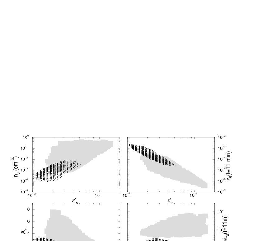
Figure 2: Grey area: parameter space (and derived quantities) for a homogeneous external medium allowed by the observed R-band flux from reverse shock (RS) at 90 seconds and from forward shock (FS) at 11 minutes, but not including the $\gamma$-ray flux during the burst. Black dots show the parameter space allowed for the observed gamma-ray flux to arise in forward shock as synchrotron emission; inverse Compton emission in FS or RS cannot account for the observed $\gamma$-ray spectrum. Top left panel shows the allowed density for the ISM ($n_{0}$) and $\epsilon^{\prime}_{e}$ (which gives the minimum LF of shock heated electrons); gray area is allowed by the early reverse shock, and late forward shock, optical observations, and black dots show the region of the parameter space permitted by GRB observation. The top right panel shows the allowed value for the magnetic field parameter $\epsilon_{B}$ in the forward shock at 11 minutes. The lower left panel shows $A_{\nu}$, a parameter that specifies the peak of the synchrotron spectrum at 11 minutes (the peak frequency is 4.95x10${}^{14}/A_{\nu}$ Hz). The lower right panel shows the ratio of $\epsilon_{B}$ in RS and FS at 11 minutes (grey region), and the ratio of $\epsilon_{B}$ in FS at deceleration time ( 3s) and at 11 minutes. Note that $\epsilon_{B}$ in RS is larger by a factor of about 10³ compared with the value in FS at 11 minutes, and $\epsilon_{B}$ in FS at deceleration is larger than at 11 minutes by a factor of about 10². ${\cal E}_{52}=30$, $t_{d}=3$s, $p=2.5$ & $z=1.0$ for all calculations; $p=2.2$ gave very similar results.

References

• (1)
• (2) Crew, G. et al. 2003, ApJ, submitted (astro-ph/0303470)
• (3) Fox, D. et al. 2003, ApJ, 586, L5
• (4) Fruchter, A. et al. 2002, GCN 1781
• (5) Greiner, J. et al. 2003, GCN 2020 reference Kobayashi, S. 2000, ApJ 545, 807
• (6) Li, W., Filippenko, A., Chornock, R. & Jha, S. 2003, ApJ, submitted (astro-ph/0302136)
• (7) Lyutikov, M. & Blandford, R.D. 2002, in β€œBeaming and Jets in Gamma-ray Bursts”, R. Ouyed, J. Hjorth & A. Nordlund, eds. astro-ph/0210671
• (8) Matheson, T. et al. 2003, GCN 2120
• (9) MΓ©szΓ‘ros , P. 2002, ARA&A 40, 137
• (10) MΓ©szΓ‘ros , P. & Rees, M.J. 1993, ApJ 405, 278
• (11) MΓ©szΓ‘ros , P. & Rees, M.J. 1997, ApJ 482, 29
• (12) Panaitescu, A. & Kumar, P. 2002, ApJ 571, 779
• (13) Panaitescu, A. & MΓ©szΓ‘ros , P., 1998, ApJ 492, 683
• (14) Panaitescu, A. & MΓ©szΓ‘ros , P., 2000, ApJ 544, L17
• (15) Piran, T. 1999, Physics Reports, 314, 575
• (16) Rees, M.J. & MΓ©szΓ‘ros , P. 1994, ApJ 430, L93
• (17) Sari, R., & Piran, T. 1999, ApJ 517, L109
• (18) Usov, V.V. 1992, Nature 357, 472
• (19) Wijers, R., Rees, M.J., & MΓ©szΓ‘ros , P. 1997, MNRAS, 288, L51
• (20) Zhang, B., Kobayashi, S. & MΓ©szΓ‘ros , P., 2003, astro-ph/0302525
• (21) Wozniak, P. et al. 2002, GCN 1757
• (22)
Refer to caption