The structure of voids

Abstract

Using high resolution $N$-body simulations we address the problem of emptiness of giant $\sim 20{h^{-1}{\rm Mpc}}$–diameter voids found in the distribution of bright galaxies. Are the voids filled by dwarf galaxies? Do cosmological models predict too many small dark matter haloes inside the voids? Can the problems of cosmological models on small scales be addressed by studying the abundance of dwarf galaxies inside voids? We find that voids in the distribution of $10^{12}\mbox{$h^{-1}$M${}_{\odot}$}$ haloes (expected galactic magnitudes $\sim M_{*}$) are almost the same as the voids in $10^{11}\mbox{$h^{-1}$M${}_{\odot}$}$ haloes. Yet, much smaller haloes with masses $10^{9}\mbox{$h^{-1}$M${}_{\odot}$}$ and circular velocities $v_{\rm circ}\sim 20~{}{{\rm km}/{\rm s}}$ readily fill the voids: there should be almost 1000 of these haloes in a $20{h^{-1}{\rm Mpc}}$–diameter void. A typical void of diameter $20{h^{-1}{\rm Mpc}}$ contains about 50 haloes with $v_{\rm circ}>50$ km/s. The haloes are arranged in a pattern, which looks like a miniature Universe: it has the same structural elements as the large-scale structure of the galactic distribution of the Universe. There are filaments and voids; larger haloes are at the intersections of filaments. The only difference is that all masses are four orders of magnitude smaller. There is severe (anti)bias in the distribution of haloes, which depends on halo mass and on the distance from the centre of the void. Large haloes are more antibiased and have a tendency to form close to void boundaries. The mass function of haloes in voids is different from the “normal” mass function. It is much steeper for high masses resulting in very few M33-type galaxies ($v_{\rm circ}\approx 100\ {{\rm km}/{\rm s}}$). We present an analytical approximation for the mass function of haloes in voids.

1 Introduction

Already more than two decades ago it became clear that large regions of the Universe are not occupied by bright galaxies (Gregory & Thompson, 1978; Joeveer et al., 1978; Kirshner et al., 1981). Large regions of size $\sim(10-20){\rm Mpc}$ devoid of galaxies can be clearly seen in all present deep redshift surveys. The observational discovery was soon followed by the theoretical understanding that voids constitute a natural outcome of structure formation via gravitational instability (Peebles, 1982; Hoffman & Shaham, 1982). Together with clusters, filaments, and superclusters, giant voids constitute the large-scale structure of the Universe. In spite of the fact that the voids are important for understanding the observed structure of the galactic distribution, they attract much less attention as compared with other elements of the large scale structure such as clusters of galaxies.

Einasto et al. (1989) were the first to estimate sizes of voids in different samples of galaxies with measured redshifts. Voids in the CfA redshift catalogs were studied by Vogeley et al. (1994). Ghigna et al. (1996) made estimates of the void probability function (VPF) for the Perseus-Pisces region. VPF was estimated for the Las Campanas redshift survey by Müller et al. (2000). El-Ad & Piran (1997, 2000) studied voids in the Optical Redshift Survey (ORS) and in the IRAS 1.2-Jy survey. They found that large voids with radius $\sim 20\mbox{$h^{-1}$Mpc}$ occupy about 50% of the volume of the Universe. Void distribution in the PSCz catalog was studied by Plionis & Basilakos (2002) and by Hoyle & Vogeley (2002) with approximately the same conclusions regarding the sizes of voids and the fraction of occupied volume. For more detailed review of observational efforts see Peebles (2001). It should be noted that in spite of significant efforts, there remain some crucial unresolved issues regarding the properties of voids. Voids are defined using bright high surface brightness galaxies. This is quite understandable: finding and measuring redshifts for dwarf or low surface brightness galaxies is difficult. For example, the absolute magnitude limit for the sample used by Vogeley et al. (1994) was $M_{B}=-19.3$ (assuming the Hubble constant $h=0.7$). The sample used by Müller et al. (2000) was limited by $M_{R}=-20$. In other words, most of the samples are probing voids using galaxies comparable with the Milky Way.

There were several attempts to find dwarf galaxies in few individual voids (Lindner et al., 1996; Popescu et al., 1997; Kuhn et al., 1997; Grogin & Geller, 1999). The overall conclusion is that faint galaxies do not show a strong tendency to fill up voids defined by bright galaxies. The limits on absolute magnitudes of observed galaxies are better than for the large samples, but not overwhelmingly so. For example, one of the voids studied by Kuhn et al. (1997) was at a distance of $\sim 3000\ {{\rm km}/{\rm s}}$, but at that distance the observational sample was complete only up to $M_{B}=-18.0$. For other voids the limit was only $M_{B}=-20.0$. The strongest arguments that voids are not populated by dwarf galaxies were given by Peebles (2001) who points out that the dwarf galaxies in the ORS catalog follow remarkably close the distribution of bright galaxies: there are no indications that they fill voids in the distribution of bright galaxies. In this case the ORS catalog can “see” galaxies with absolute magnitudes $M_{B}=-15.5$ up to 10 Mpc distance and within this distance the voids are clearly empty. A potential problem with this statement is that we do not know whether the ORS catalog is missing or not low luminosity and low surface brightness galaxies. At these magnitudes the galaxies are likely to have low surface brightnesses.

To summarize, observations indicate that large voids found in the distribution of bright $(\sim M_{*})$ galaxies are empty of galaxies, which are two magnitudes below $M_{*}$. The situation at lower limits is not clear.

Void phenomenon was a target of many theoretical studies (Einasto et al., 1991; Sahni et al., 1994; Ghigna et al., 1994; Ghigna et al., 1996; Friedmann & Piran, 2001; Arbabi-Bidgoli & Müller, 2002; Mathis & White, 2002; Benson et al., 2003; Antonuccio-Delogu et al., 2002). VPF was studied by Einasto et al. (1991) and by Ghigna et al. (1994). Our main interest is not the statistics or the shapes of the voids. We focus on the issue of emptiness of large voids. Are voids empty or are they filled with dark matter haloes? What is the structure of the dark matter distribution in voids? Does it present a problem for the standard cosmological model? These are the questions we are trying to address in this paper. Emptiness of voids is of additional interest in view of problems of the hierarchical models on small scales: the large abundance of dark matter satellites of Milky Way size haloes (Klypin et al., 1999a; Moore et al., 1999) and problems with explaining rotation curves in central parts of dwarf and low surface brightness (LSB) galaxies (e.g. Moore, 1994; Flores & Primack, 1994; de Blok et al., 2001; van den Bosch & Swaters, 2001). Both problems are on scales of $10^{9}-10^{10}\mbox{$h^{-1}$M${}_{\odot}$}$, which can be probed by the abundance of dwarf galaxies in voids.

To some degree the interest for dwarfs in voids is inspired by Peebles (2001), who claims that the CDM models have severe problems: they predict too many dwarfs. While Peebles did not try to make any quantitative estimates of the number of galaxies or dark matter haloes inside voids of large size, the reasoning seems to be simple and straightforward. At large redshifts the density in a region, which later will become a void, is not much different from the average density of the Universe at that redshift. Thus, the fluctuations grow and haloes collapse. At later times the density in the region declines and the fluctuations effectively stop growing. The number of collapsed haloes is preserved in the comoving volume of the void. This leads to a large number of expected haloes and galaxies in the void. For example, a void with a density of 1/10 of the average density of the Universe is expected to have the number density of galaxies roughly one tenth the average density of galaxies in the Universe, which gives many galaxies because of the large void volume. Mathis & White (2002) argue that gravity removes haloes from voids. That would reduce the number of haloes and galaxies. Our results show that this does not happen and thus cannot solve the problem. The simple argument of stopping the growth of fluctuations and of subsequent dilution of the halo density by void expansion must work at some scales. In that respect Peebles (2001) is right. The only question is what is the scale and what happens on larger scales.

Significant progress in understanding the void structure was made recently by Mathis & White (2002) and Benson et al. (2003), who used a combination of $N$-body simulations with semi-analytical methods to predict abundance of galaxies in voids in cosmological models. It was found that the voids are empty even of dwarf “galaxies”. Unfortunately, the mass resolution in simulations used by Mathis & White (2002) and Benson et al. (2003) is low if one wants to address the issue of dwarfs. The best simulations used by Benson et al. (2003) had the particle mass $1.4\times 10^{10}\mbox{$h^{-1}$M${}_{\odot}$}$, which leads to the minimum halo mass of few times $10^{11}\mbox{$h^{-1}$M${}_{\odot}$}$, which is not much smaller than the mass of our Milky Way galaxy. Mathis & White (2002) had better mass resolution of $3.6\times 10^{9}\mbox{$h^{-1}$M${}_{\odot}$}$ giving the minimum halo mass $3.6\times 10^{10}\mbox{$h^{-1}$M${}_{\odot}$}$. One of the goals of our paper is to extend the limit to much smaller masses to find what happens with real dwarfs in large voids. Indeed, our mass resolution is almost a hundred times better: we are able to detect haloes with mass $10^{9}\mbox{$h^{-1}$M${}_{\odot}$}$. We also develop analytical estimates of the mass function of haloes, which we test against simulations and then apply to much smaller masses.

One significant advantage of the approach used by Mathis & White (2002) and Benson et al. (2003) is that they were able to estimate luminosities of galaxies hosted by dark matter haloes. We do not try to estimate luminosities. Instead, our high resolution simulations provide the maximum circular velocities of haloes, which gives us a good idea of what kind of galaxies we are dealing with. We note that in any case the estimates of luminosities in semi-analytical models are still very uncertain for dwarf haloes: physics of these galaxies is still poorly understood. This problem is worsened by low mass resolution in the simulations of Mathis & White (2002) and Benson et al. (2003), who used haloes with as few as 10 particles to track the history of smallest galaxies. The estimates of the maximum circular velocities are better because they do not depend on what is assumed about the star formation in dwarf galaxies. Yet accurate estimates of circular velocities require high resolution $N$-body simulations: internal structure of haloes should be resolved.

In order to get a rough estimate of what luminosities may be expected for galaxies hosted by haloes in our simulations we present examples of dwarf galaxies in the Local Group, which have measured circular velocities and luminosities. If haloes in simulations host the same type of galaxies, we should expect the same luminosities. NGC 6822 and NGC 3109 are irregulars with circular velocities about $60{{\rm km}/{\rm s}}$ and absolute magnitudes $M_{B}=-15.8$ in the case of NGC 6822 (Hodge et al., 1991; Weldrake et al., 2003) and $M_{B}=-15.2$ for NGC 3109 (Mateo, 1998). For haloes with the maximum circular velocity of $60\ {{\rm km}/{\rm s}}$ the virial mass is about $(2.5-4)\times 10^{10}\mbox{$h^{-1}$M${}_{\odot}$}$ if we assume halo concentrations in the range $10-20$. For galaxies with this virial mass Mathis & White (2002) give slightly larger luminosity of $M_{B}=-16.3$. Haloes with virial mass $(2-3)\times 10^{11}\mbox{$h^{-1}$M${}_{\odot}$}$ play important role for voids. We find that voids start to fill up with haloes with masses smaller than this mass. Mathis & White (2002) give absolute magnitudes $M_{B}$ between $-17.5$ and $-18.5$ for galaxies with these virial masses. The maximum circular velocities for haloes of this mass are about $100\ {{\rm km}/{\rm s}}$, which is comparable with the circular velocity of the spiral galaxy M33 ($M_{B}=-18.5$), $v_{\rm circ}=120\ {{\rm km}/{\rm s}}$ (Corbelli & Salucci, 2000).

We investigate the formation of voids in the standard cosmological model: a spatially flat $\Lambda$-dominated Universe with scale-invariant adiabatic Gaussian fluctuations. We use the following cosmological parameters: $\Omega_{\rm M}=0.3$, $\Omega_{\Lambda}=0.7$, $\sigma_{8}=0.9$, and $h=0.7$. The age of the Universe in this model is approximately $13.5$ Gyrs. These parameters are favored by recent cosmological observations (e.g. Freedman et al. 2001; Riess et al. 2001; Spergel et al. 2003). The normalization $\sigma_{8}=0.9$ of our simulations is a rather conservative value (Bunn & White, 1997; Viana & Liddle, 1996). Some recent observational results suggest a substantially lower normalization or a lower density parameter $\Omega_{\rm M}$ (Reiprich & Böhringer, 2002; Viana et al., 2002; Bahcall et al., 2003). Pierpaoli et al. (2003) found $\sigma_{8}=0.8$, their Table 1 contains a compilation of recent estimates of $\sigma_{8}$.

The plan of the paper is as follows. In Section 2 we present our numerical simulations. We discuss briefly the void finding algorithm which we used to find voids in the distribution of dark matter haloes of a low resolution simulation and the resimulation of the regions of selected voids with a higher mass resolution. Section 3 is devoted to the formalism of analytical predictions of the mass function in voids. In Section 4 we discuss the mass and halo distribution in voids. In Section 5 we compare the analytical predictions of the mass function with the mass function measured in the high resolution simulations of voids. We discuss how the mass function depends on the normalization and a changing slope of the power spectrum as recently proposed by the WMAP collaboration (Spergel et al., 2003). Finally, in Section 6 we summarize our results.

2 Numerical models

2.1 The code

The Adaptive Refinement Tree (ART) $N$-body code of Kravtsov et al. (1997) was used to run all numerical simulations analyzed in this paper. This code uses Adaptive Mesh Refinement technique to achieve high resolution in the regions of interest. The computational box is covered with a uniform grid which defines the lowest (zeroth) level of resolution. The code then reaches high force resolution by recursively refining all high density regions using an automated refinement algorithm. The shape of the refinement mesh can thus effectively match the geometry of the region of interest. This algorithm is well suited for simulations of a selected region in a large computational box, as in the simulations presented below. During the integration, spatial refinement is accompanied by temporal refinement. Namely, each level of refinement, $l$, is integrated with its own time step $\Delta a_{l}=\Delta a_{0}/2^{l}$, where $\Delta a_{0}$ is the global time step of the zeroth refinement level. In addition to spatial and temporal refinement, simulations described below also use a non-adaptive mass refinement algorithm to increase the mass (and correspondingly the force) resolution inside a specific region (Klypin et al., 2001).

We start with running a low resolution simulation with $128^{3}$ particles covering the whole computational box. For that we make a realization of the initial spectrum of perturbations with $1024^{3}$ particles in the simulation box. Initial coordinates and velocities of the particles are then calculated using all waves ranging from the fundamental mode $k=2\pi/L$ to the Nyquist frequency $k=2\pi/L\times N^{1/3}/2$, where $L$ is the box size and $N=1024^{3}$ is the number of particles in the simulation. Then we replace every $8^{3}=512$ particles with particles of larger mass. A large-mass (merged) particle is assigned a velocity and displacement equal to the average velocity and displacement of the small-mass particles. Once a simulation with $128^{3}$ particles is completed, we select voids and identify all particles inside the voids.

Then we restart the simulation keeping high mass resolution for particles in voids. Particles outside the high resolution region are merged in several steps so that the high resolution region corresponding to $1024^{3}$ particles is surrounded by shells with resolution corresponding to $512^{3}$ and $256^{3}$ particles. The remaining part of the simulation box is simulated in low mass resolution corresponding to $128^{3}$ particles. High force resolution is only achieved inside the region with high mass resolution. The details of this multi-mass technique are described by Klypin et al. (2001).

2.2 Simulations

In order to study the formation of large voids, the simulation box should be sufficiently large; we use a cube of 80$h^{-1}{\rm Mpc}$ on a side. This is sufficient because we are not interested in a statistics of large voids, which would require a significantly larger volume. Our main interest is in the structure of a typical $\sim 10\mbox{$h^{-1}$Mpc}$–radius void. The 80$h^{-1}{\rm Mpc}$ box is large enough for that. We focus on the formation of small structural elements (haloes and filaments) inside voids, for which we need the highest possible mass resolution.

The limitation of $1024^{3}$ particles gives the $4.0\times 10^{7}\mbox{$h^{-1}$M${}_{\odot}$}$ per particle. This leads to the minimum halo mass of $10^{9}{h^{-1}M_{\odot}}$. A halo with this mass has the maximum circular velocity $\sim 20~{}{{\rm km}/{\rm s}}$. Inside the high resolution region we reach the force resolution (one cell) of $0.6{h^{-1}{\rm kpc}}$. We make 250000 time-steps on the highest resolution level.

The identification of haloes is always a challenge. The widely used halo-finding algorithms, the friends-of-friends (FOF) and the spherical overdensity, both discard “haloes inside haloes”, i.e. satellite haloes located within the virial radius of larger haloes. We have developed two algorithms that do not suffer from this drawback: the hierarchical friends-of-friends (HFOF) and the bound density maxima algorithms (BDM, see Klypin et al. 1999b).

The algorithms are complementary. They find essentially the same haloes. Thus we believe that the algorithms are stable and capable of identifying all dark matter haloes in our simulations. The advantage of the HFOF algorithm is that it can handle haloes of arbitrary shape, not just spherical haloes. The advantage of the BDM algorithm is that it describes the physical properties of the haloes better by identifying and removing unbound particles. In particular it estimates not only the mass of a halo, but also its maximum “circular velocity”, $v_{\rm circ}=\sqrt{GM/R}$. This is the quantity which is more meaningful observationally. Numerically, $v_{\rm circ}$ can be measured more easily and more accurately than the mass. In order to compare the velocity function of haloes measured in simulations with analytical predictions one has to convert the virial masses into circular velocities assuming an NFW density profile (Gottlöber et al., 1999).

2.3 Finding voids

In order to identify voids, we start with construction of the minimal spanning tree for selected haloes. Typically we select haloes with mass larger than $2\times 10^{11}\mbox{$h^{-1}$M${}_{\odot}$}$, but different criteria were also used. Then we search on a grid with mesh size $0.6{h^{-1}{\rm Mpc}}$ for the point in the simulation box which has the largest distance $R_{1}$ to the set of haloes. This is the centre of the largest void the radius of which is $R_{1}$. We exclude this void and search again for a point with the largest distance to the set. This gives the second largest void and so on. The algorithm is similar to that used by Einasto et al. (1989). El-Ad & Piran (1997) use a somewhat more complicated search algorithm based on “wall” and “field” galaxies, where field galaxies are allowed to be also in voids.

In principle, our algorithm (as the algorithm of El-Ad & Piran 1997) allows for the construction of voids with arbitrary shape: the starting point is a spherical void which can be extended by spheres of lower radius which grow from the surface of the void into all possible directions. However, in the following analysis we have restricted ourselves to spherical voids to avoid ambiguities of the definition of allowed deviations from spherical shape.

3 Analytical approximations for the mass function in a low density region

In this section we provide a formalism for predicting the mass function of dark matter haloes in voids. There are different ways of constructing the mass function in voids. Using the barrier-crossing formalism of Bond et al. (1991) and Lacey & Cole (1993), Mo & White (1996) generalized the Press-Schechter approximation so that it can be applied to over- and under-dense regions. The validity of this approach has been verified against $N$-body simulations by Lemson & Kauffmann (1999). A better approximation is provided by Sheth & Tormen (2002, ST). We compare predictions based on this approximation with our $N$-body results and find that it does not provide an accurate fit to the results of simulations. This motivates us to develop our own approximation.

For completeness, we start with presenting the constrained ST approximation. If $\rho_{\rm void}$  is the mean density of matter in a void and $\sigma(R)$ is the rms density fluctuation at comoving scale $R$, then the number density $n_{\rm c,ST}$ of haloes with mass $M(R)=4\pi\rho_{\rm b}R^{3}/3$ is given by

$$n_{\rm c,ST}(M) = -\left(\frac{2}{\pi}\right)^{1/2}\frac{\varrho_{\rm void}}{M}\frac{|T(\sigma^{2}|\sigma_{0}^{2})|}{(\sigma^{2}-\sigma_{0}^{2})^{3/2}}\frac{\sigma{\rm d}\sigma}{{\rm d}M}$$ (1)

$$\times \exp\left[-\frac{[B(\sigma^{2})-B(\sigma_{0}^{2})]^{2}}{2(\sigma^{2}-\sigma_{0}^{2})}\right]$$

where

$$T(\sigma^{2}|\sigma_{0}^{2})=\sum_{n=0}^{5}\frac{(\sigma_{0}^{2}-\sigma^{2})^{n}}{n!}\frac{\partial^{n}[B(\sigma^{2})-B(\sigma_{0}^{2})]}{\partial(\sigma^{2})^{n}}$$ (2)

(note the correction of the typo with respect to Sheth & Tormen 2002; R. Sheth, private communication). Here

$$B(\sigma^{2}) = a^{1/2}\delta_{\rm c}[1+\beta(a\delta_{\rm c}^{2}/\sigma^{2})^{-\alpha}],$$ (3)

$$B(\sigma_{0}^{2}) = a^{1/2}\delta_{0}[1+\beta(a\delta_{0}^{2}/\sigma_{0}^{2})^{-\alpha}].$$ (4)

The parameters $\alpha=0.615$, $\beta=0.485$ are given by the ellipsoidal dynamics, while $a=0.707$ is adjusted by comparison with simulations. The parameter $\delta_{0}$ is the linear underdensity of the void corresponding to the actual nonlinear underdensity at the moment at which we measure the mass function ($z=0$ in our case). It is calculated from the spherical top-hat model (Sheth & Tormen, 2002):

$$\delta_{0}(\delta) = \frac{\delta_{\rm c}}{1.68647}\left[1.68647-\frac{1.35}{(1+\delta)^{2/3}}\right.$$ (5)

$$- \frac{1.12431}{(1+\delta)^{1/2}}+\left.\frac{0.78785}{(1+\delta)^{0.58661}}\right].$$

Here $\delta$ denotes the mean density contrast in the void, $\delta=\varrho_{\rm void}/\varrho_{\rm b}-1=\Delta(R_{\rm void})/\Omega_{\rm M}-1$, where $\Delta=3M(R)/(4\pi R^{3}\varrho_{\rm c})$ is the mean density in a sphere of radius $R$. We will assume that the density in a void does not depend on the distance from the centre of the void. Later we will see that this not exactly true, but it is a reasonable starting point. In the expression above, $\varrho_{\rm b}$ is the background density, $\delta_{\rm c}$ is the characteristic density for collapse as predicted by linear theory according to the spherical collapse model (for our cosmology, $\delta_{\rm c}=1.676$, see Łokas & Hoffman 2001).

The parameter $\sigma_{0}$ is defined as the linear rms fluctuation on the scale of the void. It is estimated using the linear power spectrum and the top-hat filter with radius $R_{0}$ defined by $R_{0}^{3}=(1+\delta)R^{3}_{\rm void}$, where $R_{\rm void}$ and $\delta$ are the radius and the mean density contrast of the void. The parameter $\sigma_{0}$ is essential for this approach. It provides truncation for objects with large mass: as the amplitude of perturbation $\sigma$ approaches the amplitude of perturbation of the void, the number density of haloes goes to zero. The effect of truncation is “felt” even for much smaller objects.

The formalism of the constrained mass function in the version proposed by Sheth & Tormen (2002) is rather complicated and arbitrary in a sense that the series in equation (2) is not well motivated and the parameters of the model are adjusted by comparison with $N$-body simulations. We introduce an alternative and in our opinion much more straightforward and natural method of predicting the mass function in voids. As we will show in Section 5, it also reproduces our simulated mass functions more accurately. Our method is based on the assumption that the evolution of matter distribution in a void proceeds effectively as it would in a Universe with cosmological parameters similar to those of the void. We treat the void as a Universe with a density parameter $\Omega_{\rm M,void}=\Delta(R_{\rm void})$ with $\Delta(R_{\rm void})$ measured from the simulations.

The growth of perturbations in such a Universe is also slower than in the whole Universe. In order to take this into account we change the normalization of the power spectrum in the void by assuming a new value of $\sigma_{8,{\rm void}}$, related to the background $\sigma_{8}$ by

$$\sigma_{8,{\rm void}}=\sigma_{8}\frac{D(a_{\rm i})}{D(a=1)}\frac{D_{\rm void}(a=1)}{D_{\rm void}(a_{\rm i})}$$ (6)

where $D(a)$ and $D_{\rm void}(a)$ are the linear growth factors of density perturbations in the background and in the void respectively, normalized so that for $\Omega_{\rm M}=1$ and $\Omega_{\Lambda}=0$ we have $D(a)=a$. We assume that at some initial $a_{\rm i}=1/(1+z_{\rm i})$ $(z_{\rm i}\approx 1000)$ the rms fluctuations in the background and in the void were equal.

For a flat model with $\Omega_{\rm M}+\Omega_{\Lambda}=1$ describing our background Universe the growth factor is given (Silveira & Waga 1994, corrected for typos) by

$$D_{\rm flat}(a)=a\ \ _{2}F_{1}\left[\frac{1}{3},1,\frac{11}{6},a^{3}\frac{\Omega_{\rm M}-1}{\Omega_{\rm M}}\right]$$ (7)

where ${}_{2}F_{1}$ is a hypergeometric function. For non-flat cosmologies, such as those of the voids, $D(a)$ has to be calculated numerically using (Heath, 1977; Carroll et al., 1992) $D(a)=[5\Omega_{\rm M}/(2af(a))]\int_{0}^{a}f^{3}(a){\rm d}a$, where $f(a)=\left[1+\Omega_{\rm M}\left(\frac{1}{a}-1\right)+\Omega_{\Lambda}\left(a^{2}-1\right)\right]^{-1/2}.$ We then use unconstrained ST approximation (Sheth & Tormen, 1999) to find the mass function of haloes in voids:

$$n_{\rm ST}(M) = -\left(\frac{2}{\pi}\right)^{1/2}A\left[1+\left(\frac{a\delta_{\rm c}^{2}}{\sigma^{2}}\right)^{-p}\right]a^{1/2}$$

$$\times \frac{\varrho_{\rm b}}{M}\frac{\delta_{\rm c}}{\sigma^{2}}\frac{{\rm d}\sigma}{{\rm d}M}\exp\left(-\frac{a\delta_{\rm c}^{2}}{2\sigma^{2}}\right),$$

where $A=0.322$, $p=0.3$ and $a=0.707$. Here we take $\delta_{\rm c}=1.62$, which is appropriate for the ‘open Universe’ parameters of the voids in our simulations $\Omega_{\rm M,void}=0.03-0.05$ and $\Omega_{\Lambda}=0.7$ (see Łokas & Hoffman 2001).

4 Voids in simulations

4.1 Mass distribution in voids

Figure 1: Cumulative fraction of the volume occupied by 20 largest voids in the distribution of haloes with different limiting circular velocities. More massive haloes define slightly larger voids.

In the simulation box of size 80 $h^{-1}{\rm Mpc}$ we found 1348 dark matter haloes with circular velocities larger than 200 km/s and 2518 with circular velocities larger than 120 km/s. We search for spherical non-overlapping voids in the distribution of the dark matter haloes. The 20 largest voids have radii larger than 8.81 $h^{-1}{\rm Mpc}$ when the limiting circular velocity of haloes is set to $v_{\rm circ}>200$ km/s while larger than 8.26 $h^{-1}{\rm Mpc}$ for haloes with $v_{\rm circ}>120$ km/s. In Figure 1 we show the cumulative fraction of volume occupied by the 20 largest voids. The voids in the distribution of more massive haloes tend to be larger, but the difference is small as long as the difference in mass is not very big. A similar behaviour has been found by Arbabi-Bidgoli & Müller (2002). This indicates that there are only rare cases when a given void is divided into two parts if the threshold for the circular velocity (or mass) of the objects defining the void is reduced. This statement is supported by our conclusion that there is a tendency to find more massive haloes in the outer part of voids.

Five voids were resimulated with mass resolution $4.0\times 10^{7}{h^{-1}M_{\odot}}$. In the low resolution simulation their radii were $R_{\rm void}=11.6{{h^{-1}{\rm Mpc}}}$, $10.8{{h^{-1}{\rm Mpc}}}$, $9.4{{h^{-1}{\rm Mpc}}}$, $9.1{{h^{-1}{\rm Mpc}}}$, $9.1{{h^{-1}{\rm Mpc}}}$. With the high resolution mentioned above we resimulated regions with 10% larger radii, so that the objects which define the borders of the voids have been also resimulated. The void finding algorithm assumes point-like objects. However, these objects have a certain size. Moreover, they could be surrounded by satellites with smaller masses. Since we do not want to include in our analysis the objects themselves or their satellites (which in the sense of the definition do not belong to the void) we have assumed a void radius of 10 $h^{-1}{\rm Mpc}$ or 8 $h^{-1}{\rm Mpc}$ for the large and small voids respectively.

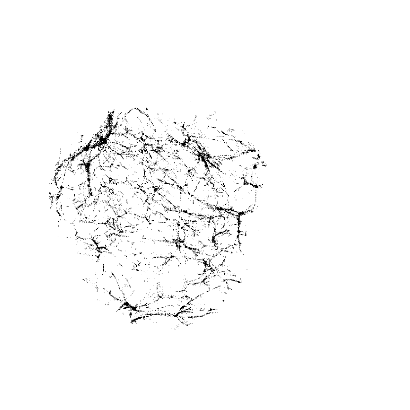
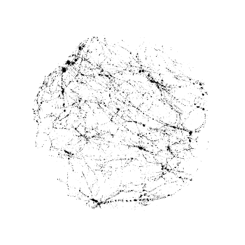
Figure 2: The distribution of dark matter inside a large void. Bottom panel shows the distribution of matter in a void with radius $10{h^{-1}{\rm Mpc}}$ at redshift $z=0$. Top: all particles belonging to the void are traced back to redshift $z=2$ and are shown in comoving coordinates. The distribution looks like normal large-scale structure in the distribution of galaxies: the haloes are in filaments, there are “voids” and most massive objects are at intersections of large filaments. Yet, the whole region is a void: there is no Milky Way size halo in the picture. Numerous knots along the filaments are haloes with masses $10^{9}\mbox{$h^{-1}$M${}_{\odot}$}$. Large haloes have masses of few times $10^{10}\mbox{$h^{-1}$M${}_{\odot}$}$.

In the bottom part of Figure 2 we show a sphere of radius 10 $h^{-1}{\rm Mpc}$ centered on the void of radius 10.8 $h^{-1}{\rm Mpc}$. This void does not contain any halo of mass greater than $2.0\times 10^{11}$ $h^{-1}M_{\odot}$. The progenitor of this void at redshift $z=2$ is not spherical. It is much smaller in comoving coordinates, i.e. the density contrast of the void with respect to the mean density was much smaller at high redshifts. Note, however, that this does not prove the statement that voids become more spherical during evolution, because the selected voids are spherical by definition at $z=0$. The void and its progenitor are shown in the same projection in comoving coordinates. The obvious shift of the centre of the void means that the void not only expands anisotropically with respect to the background but also that the whole void moves with respect to the comoving coordinate system. It is interesting to see that there is already a huge number of dense filaments at redshift $z=2$ which should be observable in the Lyman $\alpha$ forest.

Inside the void at redshift $z=0$ we find almost the same structures as seen in simulations of large parts of the Universe: empty regions, filaments and matter concentrations at the points where filaments join. However, all masses are scaled down by a factor of several orders of magnitude. In the crossing points of filaments we find instead of huge dark matter haloes hosting clusters of galaxies only small haloes which might host dwarf galaxies. Along the filaments even smaller haloes are situated. The three-dimensional distribution of matter seems to be non-uniform. Large nodes of filaments seem to be situated nearer to the border of the void than to its centre. This visual impression is supported by the distribution of dark matter (cf. Figure 3) and haloes (cf. Figure 4).

Figure 3: The mean density in spheres of radius $R$ centered on the centre of each of the five voids. The two thick solid lines denote the voids with radius $10{h^{-1}{\rm Mpc}}$, the three thin solid lines denote voids with radius $8{h^{-1}{\rm Mpc}}$.

Let us first consider the mean density in spheres centered at the void’s centre. We express the mean density in units of the critical density, i.e. in a way similar to the (constant) $\Omega$ parameter: $\Delta=3M(R)/(4\pi R^{3}\varrho_{\rm c})$ where $M(R)$ is the total mass inside a sphere of radius $R$ centered at the centre of the void and $\varrho_{\rm c}$ is the critical density. As one can see in Figure 3, inside a void the density increases slightly with radius and is typically a factor of 10 smaller than the mean density $\Omega_{\rm M}=0.3$. Our voids have smaller densities than those described by Friedmann & Piran (2001), who found that voids typically have half the mean density.

Large differences can be seen in the environment of voids. Most of the voids are situated in regions of low density. Up to the radius of 30 $h^{-1}{\rm Mpc}$ the mean density in the spheres is still well below the mean density of the Universe. However, the most prominent structure of the simulation, a galaxy cluster of mass $2\times 10^{15}{h^{-1}M_{\odot}}$, is close to void 4. Therefore, the density outside this void rapidly increases so that the mean density of a sphere of radius 20 $h^{-1}{\rm Mpc}$ centered on this void is already well above $\Omega_{\rm M}=0.3$. On the contrary, the most prominent clusters in the box are at distances of 51 $h^{-1}{\rm Mpc}$ resp. 47 $h^{-1}{\rm Mpc}$ from the center of void 5. Therefore, the mean density in spheres centered on the centre of void 5 remains below 0.2 up to radii 30 $h^{-1}{\rm Mpc}$ and reaches 0.3 only for radii above 50 $h^{-1}{\rm Mpc}$ . We did not find any significant differences in the inner structure of the voids so we conclude that the environment of the voids has no influence on the void itself.

4.2 Haloes in voids

Visual inspection of the void simulations shows plenty of haloes in the void. In Section 2 we have described how haloes can be identified in dark matter simulations. At first glance we can see that haloes are not homogeneously distributed in the void (Figure 2), large haloes seem to be concentrated in the outer parts of the void. We want to quantify this statement.

We divided our sample of haloes in the five voids into two subsamples containing 164 haloes with circular velocities 55 km/s $<v_{\rm circ}<120$ km/s and 207 haloes with circular velocities 20 km/s $<v_{\rm circ}<55$ km/s. Each void was divided into five shells of equal volume. In Figure 4 we show the mean number density of haloes in the five shells the radius of which is normalized to the void radius. The thick line in the Figure corresponds to the haloes with higher circular velocities, while the thin one to those with lower velocities. One can clearly see that there is a tendency for the haloes to concentrate more at the outer parts of the voids. This tendency is more pronounced for the more massive haloes (thick line), their density in the outer shell is almost a factor of three higher than in the central sphere.

Figure 4: Mean number density of haloes with circular velocities 55 km/s $<v_{\rm circ}<120$ km/s (thick line) and 20 km/s $<v_{\rm circ}<55$ km/s (thin line) in shells of equal volume ($V_{\rm void}/5$) for five voids. The radius of the shell is normalized to the void radius.

Down to the limit of $10^{9}\mbox{$h^{-1}$M${}_{\odot}$}$ we find thousands of haloes in the simulation. Now we are interested in the mass function of haloes in different voids and its dependence on the mean density in the void. We select all haloes inside the assumed void radius $R_{\rm void}=10{h^{-1}{\rm Mpc}}$ or $R_{\rm void}=8{h^{-1}{\rm Mpc}}$ depending on the void and estimate the mass function of haloes in each of the voids. Figure 5 shows the five mass functions measured in the five simulated voids. The mean dark matter density in the voids (see Figure 3) is about $\Delta(R_{\rm void})=0.03$ for the larger voids with $R_{\rm void}=10{h^{-1}{\rm Mpc}}$ and $\Delta(R_{\rm void})=0.04$ for the smaller voids with $R_{\rm void}=8{h^{-1}{\rm Mpc}}$.

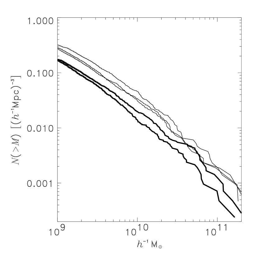
Figure 5: Mass functions of haloes in five simulated voids. The two thick solid lines correspond to voids with radius $R_{\rm void}=10{h^{-1}{\rm Mpc}}$ and mean density $\Delta(R_{\rm void})=0.03$, while the three thin solid lines denote voids with radius $R_{\rm void}=8{h^{-1}{\rm Mpc}}$ and mean density $\Delta(R_{\rm void})=0.04$ (see Figure 3).

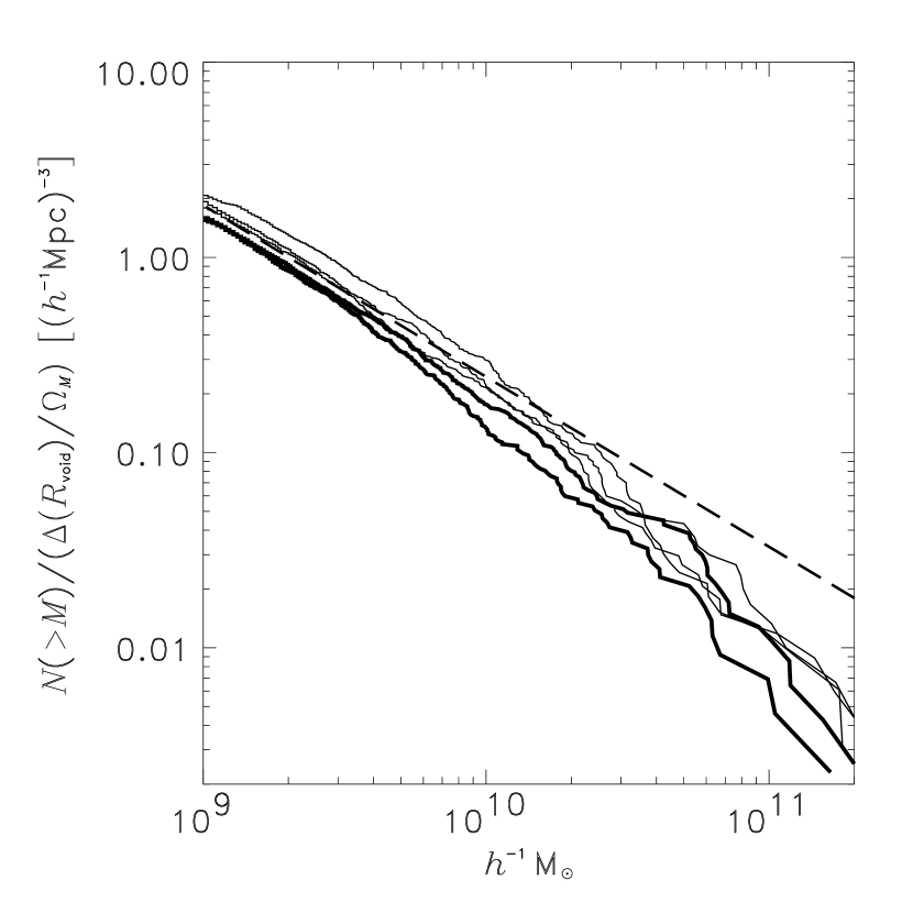
Figure 6: The same mass functions as in Figure 5 but scaled by $\Delta(R_{\rm void})/\Omega_{\rm M}$. The dashed line denotes the mass function of the field according to the Sheth-Tormen formalism, thin and thick solid lines correspond to voids with different radii as in Fig. 5.

The different mean (under)densities of the simulated voids result in different mass functions. The higher the density in voids the higher is also the number density of haloes. The number density of haloes in voids is about an order of magnitude smaller than in the whole box as expected due to mean density in voids which is also about an order of magnitude smaller (Gottlöber et al., 2002). This can be also seen in Figure 6 where we have shown the mass function of field haloes obtained by the Sheth-Tormen formalism. This mass function is in excellent agreement with the mass function measured in the whole 80 $h^{-1}{\rm Mpc}$ box (Gottlöber et al., 2002). In Figure 6 we have scaled the mass functions in voids with the mean density contrast measured in the void with respect to the mean density of matter in the universe, $\Delta(R_{\rm void})/\Omega_{\rm M}$. Now the scatter between the mass functions of the different voids is smaller. Note, that the shape of the mass function in voids is steeper than in the whole box. One can clearly see that after rescaling the overall mass function with the density in voids, the less massive halos are as abundant in voids as the general mass function predicts. The more massive halos, on the other hand, are deficient in the voids.

5 The mass function in voids

5.1 Comparison of simulated and analytical mass functions

The top panel of Figure 7 shows predictions obtained using constrained Sheth-Tormen mass function equations (1)-(4) with $\Delta(R_{\rm void})=0.05,0.04,0.03$ and assuming the size of the void $R_{\rm void}=10h^{-1}$ Mpc (smaller sizes of voids result in steeper mass functions). The analytical results presented here differ from those of Gottlöber et al. (2002) in that they assumed $a=0.5$ in equations (3)-(4) to fit the simulated mass function better while here we keep the value $a=0.707$ advertised by Sheth and Tormen everywhere. The constrained mass functions do not provide good fits to the $N$-body results. They are too steep and are a factor of 2–10 below the simulations. They are especially bad for voids with very low densities.

In the bottom panel in Figure 7 we compare the simulated mass functions with the predictions based on rescaled mass function given by equation (3). To make the analytical predictions we use the same values of the mean density as in the simulated voids: $\Omega_{\rm M,void}=\Delta(R_{\rm void})=0.05,0.04,0.03$. For voids with these densities we get the corrected values for the normalization of the power spectrum $\sigma_{8,{\rm void}}=0.25,0.20,0.14$ respectively. It is clear that the rescaled mass functions provide much better fits to the simulations. Yet, the fits are not very accurate. One may try to improve the fits by changing parameters $A$, $p$ and $a$ in equation (3). After all, values of these parameters to some extent were tuned to fit $N$-body simulations. However, this is not a good way to improve the approximation: predictions are quite stable. For example, the values of $A$, $p$ and $a$ suggested by Jenkins et al. (2001) do not change our results significantly and do not produce better agreement with simulations.

Figure 7: Comparison of the mass functions in five simulated voids (thin and thick solid lines correspond to voids with different radii as in Fig. 5) to the predictions (dashed lines) based on constrained ST mass function (top panel) and rescaling the unconstrained ST mass function (bottom panel). The dashed curves from the highest to the lowest are for $\Delta(R_{\rm void})=\Omega_{\rm M,void}=0.05,0.04,0.03$.

Figure 8: The solid curves are mass functions in simulations of voids. Void radii are reduced by 20% as compared with the void radii in Fig. 5. The two thick solid lines correspond here to the radius $R_{\rm void}=8{h^{-1}{\rm Mpc}}$, while the three thin solid lines correspond to the radius $R_{\rm void}=6.4{h^{-1}{\rm Mpc}}$. Dashed curves show predictions from the rescaled ST mass functions for $\Omega_{\rm M,void}=0.03$ and $0.04$. The analytical predictions and numerical results are now in a very good agreement.

The low accuracy of the approximation can be traced to the fact that we assume a constant density of the dark matter inside a void. At the same time simulated voids have density, which visibly increases close to the void boundaries. The number density of haloes (especially massive ones) is very sensitive to the average dark matter density as clearly illustrated by Figure 4. This inconsistency in treatment of the voids is the main reason for poor quality of the fits. The tendency of more massive haloes to concentrate in the outer part of the voids is also in agreement with the slowly increasing cumulative volume fraction of voids defined by samples of haloes with different minimum circular velocities (cf. Figure 1). In fact, if those haloes were uniformly distributed one would more often expect that one of the big voids will be divided into two smaller ones if one decreases the threshold of the halo mass or circular velocity defining the voids. This is not the case as one can see from the small differences in the volumes of the largest voids defined in the set of haloes with different circular velocities (see Figure 1).

In order to reduce the effect of the varying density, we find the simulated halo mass function using void radii which are 20% smaller than their actual radii. Figure 8 shows the results. The full curves represent the mass functions measured in the five voids with the reduced radii. They are now steeper at the high mass end. The dashed curves show the predictions based on the rescaled Sheth-Tormen approximation (the same as in the bottom panel of Figure 7). The agreement between the analytical predictions and numerical results is now significantly improved.

5.2 Dependence of the halo mass function in voids on different parameters

Even now the normalization of the power spectrum of density perturbations has some uncertainties. Observational constraints before recent WMAP results give uncertainty of about 10% for the parameter $\sigma_{8}$ (see Bahcall et al. 2003 for SDSS estimates and for a discussion of other measurements which have a tendency to predict low values of $\sigma_{8}$). However, the WMAP results (Bennett et al., 2003) again favour $\sigma_{8}=0.9$ if the perturbation spectrum is scale invariant with $n=1$. The mass function in voids is affected by all these uncertainties: it becomes steeper with decreasing normalizations of the background power spectrum (with other cosmological parameters unchanged).

Figure 9: Rescaled ST mass function for $\Omega_{\rm M,void}=0.04$ and $\sigma_{8}=0.9$ (dashed line) in comparison to the mass function obtained for $\sigma_{8}=0.84$ and scale-dependent spectral index $n=0.93-0.031\ln(k/k_{0})$ (solid line) as proposed by WMAP (Spergel et al., 2003).

The combination of WMAP results with other CMB measurements, 2dF and Lyman $\alpha$ forest results indicate a lower normalization of $\sigma_{8}=0.84$ together with a scale-dependent slope of the primordial power spectrum $n=0.93-0.031\ln(k/k_{0})$ with $k_{0}=0.05$ Mpc^-1 (Spergel et al., 2003). Using these parameters we apply the rescaled ST approximation to estimate the halo mass function in voids. Figure 9 shows the estimates. As expected, the mass function is then less steep than the mass functions with the same normalization and a constant slope $n=1$. On the other hand, decreased normalization makes it steeper so the net effect is that it is just shifted down with respect to the mass function found for $\sigma_{8}=0.9$ and $n=1$.

Note, that in Figure 9 the mass function is shown down to $10^{7}\mbox{$h^{-1}$M${}_{\odot}$}$. This is far beyond the range which can be tested in a numerical experiment, but due to the good agreement between the numerical simulation and the analytical approach we expect that the rescaled ST mass function can be extended to smaller masses. Using this approximation we predict that in a typical void of diameter $\sim 20{h^{-1}{\rm Mpc}}$ there should be about 100 000 objects of mass greater than $10^{7}\mbox{$h^{-1}$M${}_{\odot}$}$. It is a challenge to observers to confirm this prediction. Recently, the existence of a large population of hydrogen clouds in voids has been claimed (Manning, 2002). These clouds could be associated with a fraction of the numerous haloes which we found in the simulated voids.

The expected number of dark matter haloes of different mass depends on the void (under)density. In Figure 10 we show predictions for the number of haloes inside a typical void of radius $10\mbox{$h^{-1}$Mpc}$ for haloes with mass larger than $10^{12}\mbox{$h^{-1}$M${}_{\odot}$}$, $10^{10}\mbox{$h^{-1}$M${}_{\odot}$}$ and $10^{8}\mbox{$h^{-1}$M${}_{\odot}$}$ as functions of the average density of the void. There is a dramatic decline in the number of haloes when the average density of the void falls below a certain percentage of the mean density. The larger the mass of the haloes, the larger is the void density at which the sharp decline happens. This decline is related to the steepening of the void mass function at the high mass end as seen in Figure 6. Note, that for typical voids with the average density ten times below the mean density, the number of $10^{8}\mbox{$h^{-1}$M${}_{\odot}$}$ haloes is not yet suppressed: the sharp decline is at lower average densities.

Figure 10: The number of haloes with the virial mass larger than $10^{12}\mbox{$h^{-1}$M${}_{\odot}$}$ (bottom curve), $10^{10}\mbox{$h^{-1}$M${}_{\odot}$}$ (middle curve), and $10^{8}\mbox{$h^{-1}$M${}_{\odot}$}$ (top curve) inside a typical void of radius $10\mbox{$h^{-1}$Mpc}$ as a function of the average density of the void $\Omega_{\rm void}$. These predictions come from the rescaled unconstrained mass function. A “void” with $\Omega_{\rm void}=0.3$ has the average matter density in the Universe.

6 Discussion and conclusions

We used $N$-body simulations to study the formation of voids in the large-scale structure of the Universe. We first identified dark matter haloes and then searched for voids in the distribution of the haloes. We found that the size of the voids depends weakly on the lower mass (or circular velocity) limit of the haloes chosen to define the void. Voids in a set of more massive haloes tend to be slightly larger than voids in a set of smaller haloes.

The interior of five largest voids was resimulated with very high mass resolution of $4\times 10^{7}{h^{-1}M_{\odot}}$. These voids have diameters of about $20\mbox{$h^{-1}$Mpc}$ and their density is about a factor of 10 smaller than the mean density in the Universe. Inside a void of this size we found typically about 50 haloes with circular velocities larger than 50 km/s and more than 800 with circular velocities larger than 20 km/s. A scale-dependent slope of the primordial power spectrum as recently suggested by Spergel et al. (2003) would slightly reduce the number of low mass haloes in voids.

Mathis & White (2002) find “several void regions with diameter $10{h^{-1}{\rm Mpc}}$ in the simulations where gravity seems to have swept away even the smallest haloes” they “were able to track”. According to their Table 1 they tracked haloes down to 10 particles corresponding to halo masses $3.6\times 10^{10}{h^{-1}M_{\odot}}$. In our simulations of voids of diameter $20{h^{-1}{\rm Mpc}}$ we find typically up to 10 haloes of this mass (represented by 1000 particles). More than half of the haloes are close to the outer void boundary with a distance to the void’s centre larger than 80% of the void’s radius. Since our void volume is 8 times larger and more massive haloes tend to be situated in the outer part of the void it would be not extremely unprobable to find inside our voids regions of $10{h^{-1}{\rm Mpc}}$ free of any halo more massive than $3.6\times 10^{10}{h^{-1}M_{\odot}}$. In this respect we agree with Mathis & White (2002). Following the evolution of voids numerically it seems that these haloes are not swept away by gravity but never form in regions with the lowest density.

The fact that regions devoid of haloes with masses larger than $5\times 10^{10}{h^{-1}M_{\odot}}$ are smaller than those devoid of haloes with masses bigger than $2\times 10^{11}{h^{-1}M_{\odot}}$ emphasizes our argument that the size of the voids depends on the objects used to define the void. For example, the voids in the distribution of clusters are not empty: they contain many $L_{*}$ galaxies. Likewise, the voids in a sample of $L_{*}$ galaxies should contain dwarfs. This argument suggests that voids in the dark matter distribution should be self-similar in the same sense as clusters of galaxies have hundreds of galaxies and galaxies have hundreds of satellites. It must be so as long as only the gravity is the dominant factor and the spectrum of fluctuations is approximately scale invariant. The question whether luminous galaxies form or do not form in all these dark matter haloes is then the most important question in the theory of galaxy formation in different environments.

Assuming with Mathis & White (2002) a luminosity $M_{B}=-16.5$ for a galaxy hosted by a halo of $3.6\times 10^{10}{h^{-1}M_{\odot}}$ we predict about five of these galaxies to be found in the inner part of a typical void of diameter $20{h^{-1}{\rm Mpc}}$. In principle they can be detected. In the giant (radius 31.5 Mpc) Boötes void Szomoru et al. (1996) study void galaxies in about 1% of the void volume. All but one of them were substantially brighter than $M=-16.5$. The one reported with $M=-16.2$ is the companion of a brighter one. To compare the model predictions with observations one would have to study a void in the distribution of galaxies with limiting magnitude $M_{B}$ between $-17.5$ and $-18.5$ which roughly corresponds to our threshold mass of $2\times 10^{11}{h^{-1}M_{\odot}}$.

Note, that so far we assumed that each dark matter halo hosts a galaxy. This may not be true. Physical processes of galaxy formation are not well known and there could be processes that strongly suppress the formation of stars inside small haloes, which collapse relatively late in voids. One such process which has been widely discussed is the ionizing flux (e.g. Bullock et al. 2000; Benson et al. 2002).

We determined the mass function of dark matter haloes in the simulated voids and compared it with the analytical predictions based on the Sheth-Tormen formalism. The formalism was applied in two versions: (1) We used the ansatz for the constrained mass function proposed by Sheth & Tormen (2002) and (2) we proposed our own extension of the unconstrained mass function of Sheth & Tormen (1999) by rescaling the power spectrum in the void. We found that our approach is not only much simpler in application, but also reproduces more accurately the mass functions obtained in the simulations of voids.

References

- Antonuccio-Delogu et al. (2002) Antonuccio-Delogu V., Becciani U., van Kampen E., Pagliaro A., Romeo A. B., Colafrancesco S., Germaná A., Gambera M., 2002, MNRAS, 332, 7
- Arbabi-Bidgoli & Müller (2002) Arbabi-Bidgoli S., Müller V., 2002, MNRAS, 332, 205
- Bahcall et al. (2003) Bahcall N. A., Dong F., Bode P., Kim R., Annis J., McKay T. A., Hansen S., Schroeder J., Gunn J., Ostriker J. P., Postman M., Nichol R. C., Miller C., Goto T., Brinkmann J., Knapp G. R., Lamb D. O., Schneider D. P., Vogeley M. S., York D. G., 2003, ApJ, 585, 182
- Bennett et al. (2003) Bennett C., Halpern M., Hinshaw G., WMAP collaboration 2003, astro-ph/0302207
- Benson et al. (2002) Benson A., Lacey C. G., Baugh C. M., Cole S., Frenk C. S., 2002, MNRAS, 333, 156
- Benson et al. (2003) Benson A., Hoyle F., Torres F., Vogeley M., 2003, MNRAS, 340, 160
- Bond et al. (1991) Bond J. R., Cole S., Efstathiou G., Kaiser N., 1991, ApJ, 379, 440
- Bullock et al. (2000) Bullock J. S., Kravtsov A. V., Weinberg D. H., 2000, ApJ, 539, 517
- Bunn & White (1997) Bunn E. F., White M., 1997, ApJ, 480, 6
- Carroll et al. (1992) Carroll S. M., Press W. H., Turner E. L., 1992, ARA&A, 30, 499
- Corbelli & Salucci (2000) Corbelli E., Salucci P., 2000, MNRAS, 311, 441
- de Blok et al. (2001) de Blok W. J. G., McGaugh S. S., Bosma A., Rubin V. C., 2001, ApJ, 552, L23
- Einasto et al. (1989) Einasto J., Einasto M., Gramann M., 1989, MNRAS, 238, 155
- Einasto et al. (1991) Einasto J., Einasto M., Gramman M., Saar E., 1991, ApJ, 248, 593
- El-Ad & Piran (1997) El-Ad H., Piran T., 1997, ApJ, 491, 421
- El-Ad & Piran (2000) El-Ad H., Piran T., 2000, MNRAS, 313, 553
- Flores & Primack (1994) Flores R. A., Primack J. R., 1994, ApJ, 427, L1
- Freedman et al. (2001) Freedman W. L., Madore B. F., Gibson B. K., Ferrarese L., Kelson D. D., Sakai S., Mould J. R., Kennicutt R. C., Ford H. C., Graham J. A., Huchra J. P., Hughes S. M. G., Illingworth G. D., Macri L. M., Stetson P. B., 2001, ApJ, 553, 47
- Friedmann & Piran (2001) Friedmann Y., Piran T., 2001, ApJ, 548, 1
- Ghigna et al. (1996) Ghigna S., Bonometto S. A., Retzlaff J., Gottlöber S., Murante G., 1996, ApJ, 469, 40
- Ghigna et al. (1994) Ghigna S., Borgani S., Bonometto S. A., Guzzo L., Klypin A., Primack J., Giovanelli R., Haynes M., 1994, ApJ, 437, 71
- Gottlöber et al. (1999) Gottlöber S., Klypin A. A., Kravtsov A. V., 1999, in ASP Conf. Ser. 176: Observational Cosmology: The Development of Galaxy Systems Halo evolution in a cosmological environment. p. 418
- Gottlöber et al. (2002) Gottlöber S., Łokas E., Klypin A., 2002, astro-ph/0207487
- Gregory & Thompson (1978) Gregory S. A., Thompson L. A., 1978, ApJ, 222, 784
- Grogin & Geller (1999) Grogin N. A., Geller M. J., 1999, AJ, 118, 2561
- Heath (1977) Heath D. J., 1977, MNRAS, 179, 351
- Hodge et al. (1991) Hodge P., Smith T., Eskridge P., MacGillivray H., Beard S., 1991, ApJ, 379, 621
- Hoffman & Shaham (1982) Hoffman Y., Shaham J., 1982, ApJ, 262, L23
- Hoyle & Vogeley (2002) Hoyle F., Vogeley M. S., 2002, ApJ, 566, 641
- Jenkins et al. (2001) Jenkins A., Frenk C. S., White S. D. M., Colberg J. M., Cole S., Evrard A. E., Couchman H. M. P., Yoshida N., 2001, MNRAS, 321, 372
- Joeveer et al. (1978) Joeveer M., Einasto J., Tago E., 1978, MNRAS, 185, 357
- Kirshner et al. (1981) Kirshner R. P., Oemler A., Schechter P. L., Shectman S. A., 1981, ApJ, 248, L57
- Klypin et al. (1999a) Klypin A., Kravtsov A. V., Valenzuela O., Prada F., 1999a, ApJ, 522, 82
- Klypin et al. (1999b) Klypin A., Gottlöber S., Kravtsov A. V., Khokhlov A. M., 1999b, ApJ, 516, 530
- Klypin et al. (2001) Klypin A., Kravtsov A. V., Bullock J. S., Primack J. R., 2001, ApJ, 554, 903
- Kravtsov et al. (1997) Kravtsov A. V., Klypin A. A., Khokhlov A. M., 1997, ApJS, 111, 73
- Kuhn et al. (1997) Kuhn B., Hopp U., Elsässer H., 1997, A&A, 318, 405
- Lacey & Cole (1993) Lacey C., Cole S., 1993, MNRAS, 262, 627
- Lemson & Kauffmann (1999) Lemson G, Kauffmann G., 1999, MNRAS, 302, 111
- Lindner et al. (1996) Lindner U., Einasto M., Einasto J., Freudling W., Fricke K., Lipovetsky V., Pustilnik S., Izotov Y., Richter G., 1996, A&A, 314, 1
- Łokas & Hoffman (2001) Łokas E. L., Hoffman Y., 2001, in Spooner N. J. C., Kudryavtsev V., eds, Proc. 3rd International Workshop, The Identification of Dark Matter. World Scientific, Singapore, p. 121
- Manning (2002) Manning C. V., 2002, ApJ, 547, 599
- Müller et al. (2000) Müller V., Arbabi-Bidgoli S., Einasto J., Tucker D., 2000, MNRAS, 318, 280
- Mateo (1998) Mateo M. L., 1998, ARA&A, 36, 435
- Mathis & White (2002) Mathis H., White S. D. M., 2002, MNRAS, 337, 1193
- Mo & White (1996) Mo H. J., White S. D. M., 1996, MNRAS, 282, 347
- Moore (1994) Moore B., 1994, Nature, 370, 629
- Moore et al. (1999) Moore B., Ghigna S., Governato F., Lake G., Quinn T., Stadel J., Tozzi P., 1999, ApJ, 524, L19
- Peebles (1982) Peebles P. J. E., 1982, ApJ, 257, 438
- Peebles (2001) Peebles P. J. E., 2001, ApJ, 557, 495
- Pierpaoli et al. (2003) Pierpaoli E., Borgani S., Scott D., White M. 2003, MNRAS, in press (astro-ph/0210567)
- Plionis & Basilakos (2002) Plionis M., Basilakos S., 2002, MNRAS, 330, 399
- Popescu et al. (1997) Popescu C. C., Hopp U., Elsässer H., 1997, A&A, 325, 881
- Reiprich & Böhringer (2002) Reiprich T. H., Böhringer H., 2002, ApJ, 567, 716
- Riess et al. (2001) Riess A. G., Nugent P. E., Gilliland R. L., Schmidt B. P., Tonry J., Dickinson M., Thompson R. I., Budavári T., Casertano S., Evans A. S., Filippenko A. V., Livio M., Sanders D. B., 2001, ApJ, 560, 49
- Sahni et al. (1994) Sahni V., Sathyaprakah B. S., Shandarin S. F., 1994, ApJ, 431, 20
- Sheth & Tormen (1999) Sheth R. K., Tormen G., 1999, MNRAS, 308, 119
- Sheth & Tormen (2002) Sheth R. K., Tormen G., 2002, MNRAS, 329, 61
- Silveira & Waga (1994) Silveira V., Waga I., 1994, Phys. Rev. D, 50, 4890
- Spergel et al. (2003) Spergel D., Verde L., Peiris H., WMAP collaboration 2003, astro-ph/0302209
- Szomoru et al. (1996) Szomoru A., van Gorkom J. H., Gregg M. D., 1996, AJ, 111, 2141
- van den Bosch & Swaters (2001) van den Bosch F. C., Swaters R. A., 2001, MNRAS, 325, 1017
- Viana & Liddle (1996) Viana P. T. P., Liddle A. R., 1996, MNRAS, 281, 323
- Viana et al. (2002) Viana P. T. P., Nichol R. C., Liddle A. R., 2002, ApJ, 569, L75
- Vogeley et al. (1994) Vogeley M. S., Geller M. J., Park C., Huchra J. P., 1994, AJ, 108, 745
- Weldrake et al. (2003) Weldrake D. T. F., de Blok W. J. G., Walter F., 2003, MNRAS, 340, 12