Chapter 1 Pierre Auger Atmosphere-Monitoring Lidar System

Abstract

The fluorescence-detection techniques of cosmic-ray air-shower experiments require precise knowledge of atmospheric properties to reconstruct air-shower energies. Up to now, the atmosphere in desert-like areas was assumed to be stable enough so that occasional calibration of atmospheric attenuation would suffice to reconstruct shower profiles. However, serious difficulties have been reported in recent fluorescence-detector experiments causing systematic errors in cosmic ray spectra at extreme energies. Therefore, a scanning backscatter lidar system has been constructed for the Pierre Auger Observatory in Malargüe, Argentina, where on-line atmospheric monitoring will be performed. One lidar system is already deployed at the Los Leones fluorescence detector (FD) site and the second one is currently (April 2003) under construction at the Coihueco site. Next to the established ones, a novel analysis method with assumption on horizontal invariance, using multi-angle measurements is shown to unambiguously measure optical depth, as well as absorption and backscatter coefficient.

1. Introduction

The error in shower energy estimation is directly proportional to the uncertainty in the optical depth between the fluorescence-light origin (within the extensive air shower) and FD cameras [5]. Although reasonable predictions can be obtained using atmospheric models (e.g. US Standard Atmosphere), they do not satisfactorily cover seasonal variations nor occurrence of aerosol layers, typically accompanying windy days and reaching up to 3 km over the ground. As a calorimeter of the FD, atmosphere thus requires on-line or at least periodic monitoring of its optical properties. The lidar seems to be a reasonable choice for this task and it is adopted not only by the Pierre Auger project but apparently also by other cosmic-ray related experiments [4]. In the following sections construction and analysis methods used for the reconstruction of the lidar signal are presented.

2. DAQ System

The Pierre Auger lidar system is based on the BigSky Ultra, frequency tripled Nd:YaG laser, which is able to transmit up to 20 pulses per second, each with energy of 7 mJ and 4 ns duration (i.e. pulse length 1.2 m). The emitted wavelength of 355 nm is in the $300-400$ nm range of the nitrogen fluorescence spectrum. The three receiver telescopes were constructed using $80$ cm diameter parabolic mirrors with focal length of 41 cm. The mirror is made of aluminum-coated pyrex and protected with SiO₂. The backscattered light is detected by a Hammamatsu R7400 photomultiplier with operating voltage up to 1000 V and gain up to $10^{7}$. To suppress background, a broadband UG-1 filter with 60% transmittance at 353 nm and FWHM of 50 nm is used. The distances between laser beam and the mirror centers are $\sim 1$ m, and the entry point of the laser beam into the telescope’s field of view is at $\sim 200$ m. The whole system is fully steerable with $0.1^{\circ}$ angular step. The signal is digitized using a three-channel Licel transient recorder TR40-160 with 12 bit resolution at 40 MHz sampling rate with 16k trace length combined with 250 MHz photon-counting system. Maximum detection range of the hardware is thus, with this sampling rate and trace length, set to 60 km. However, in optimal conditions atmospheric features only up to 30 km are observed. In order to limit the huge dynamic range of the lidar signal the laser is operated at 20% of the maximal energy with additional 10% attenuation filter in the beam. Schematic view of the whole DAQ system can be seen in Fig. 1–left. Typical lidar signal is shown in Fig. 1–right. Photon counting channel of the digitizer is a useful capability that can substantially extend the range for faint signals and circumvent possible inaccuracy of the analog channel.

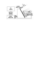
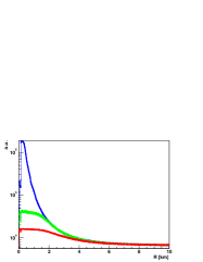
Fig. 1.: Schematic view of the lidar system (left). Example of the typical lidar signal in a.u. as a function of range $R=ct/2$ (right). Top curve: analog channel, bottom: photon counting channel (fitted to the analog channel within 5 and $10\,$km), and middle curve: fitted photon channel with dead-time correction.

3. Analysis

So called lidar equation [1,2,3], describing returned photon flux, in fact represents an under-determined system of nonlinear equations. Therefore, explicit solution of the equation does not exist. In order to obtain some useful results, certain assumptions on optical properties have to be made. One way is to postulate simple potential expression relating the backscatter coefficient $\beta$ to the attenuation (extinction) $\alpha$, as used by the Klett method [1]. In the case of the Fernald method [2], both optical properties are separated into molecular and aerosol part. Molecular part, i.e. Rayleigh scattering, is approximated with the assumed atmospheric model, and the lidar equation is solved for the aerosol part.

In Fig. 2, Fernald method is applied on the representative measurement taken with the Los Leones lidar station of the Pierre Auger observatory. Integration of the attenuation $\alpha(h)$ results in vertical optical depth (VOD) $\tau$ that directly enters estimation of the amount of fluorescence light [5], as measured by the FD. Due to the aerosol layer near the ground (in Fig. 2–left reaching up to 1.5 km) the resulting VOD clearly differs from the predictions of the (clean) atmosphere model (solid line). Judging from Fig. 2–right, the difference $\Delta\tau$ between the atmospheric model prediction and the result of the Fernald method can be as high as several tenths of the unit. Neglecting such differences produces a systematic underestimation of the shower energy (and correspondingly the energy of primary particle), since in the first order $\Delta E\propto\Delta\tau$.

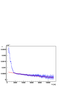
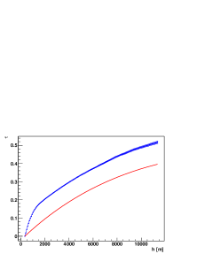
Fig. 2.: Total (molecular and aerosol) attenuation coefficient $\alpha(h)$ obtained with Fernald inversion of a vertical shot of the Los Leones lidar (left). Corresponding vertical optical depth $\tau(h)$, (right). For comparison, attenuation and optical depth as predicted by the US Standard Atmosphere (1976) model are drawn in solid line.

Due to the fairly calm and stratified atmosphere above the huge plane (Pampa Amarilla) where the Pierre Auger observatory is placed, adequate assumption of the horizontal invariance can be made. Under such an assumption the lidar equation is solved in a unique way with the two- or multi-angle method [3] for both quantities, the backscatter coefficient and the VOD measured relative to some reference height ($h_{0}$, common in all lidar signals taken at different angles). In Fig. 3, multi-angle reconstructions of simultaneous lidar signals from two telescopes in the case of relatively clear atmosphere is compared to the predictions of the atmospheric model. Note, that the relative backscatter coefficient is proportional to the relative atmospheric density, so that lidar system can also serve as a monitoring tool for the atmospheric grammage, important for the description of lateral shower development.

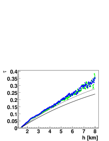
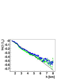
Fig. 3.: Vertical optical depth $\tau(h)$ (left) and relative backscatter coefficient $\ln\beta(h)/\beta_{0}$ (right) obtained with multi-angle analysis of lidar scans. Points are reconstructions of simultaneous signals from two telescopes, solid line represents prediction of the US Standard Atmosphere (1976) model, dashed: the same model with depolarization effects included.

4. Conclusion

Aerosol layers near ground, occurrence of haze/clouds, and in a lesser way seasonal fluctuations greatly influence shower energy estimation as obtained by the FD measurements. Periodic monitoring of this sensitive properties is thus unavoidable for any type of detection of the fluorescence light originating from air showers in large atmospheric volumes. Steerable lidar system can be successfully used for such a demanding task. Nevertheless, careful selection, optimization, and calibration of the corresponding lidar analysis methods is strongly adverted.

References

1. Klett J.D. 1981, Appl. Opt. 20, 211

2. Fernald F.G. 1984, Appl. Opt. 23, 652

3. Filipčič A. et al. 2003, Astropart. Phys. 18, 501

4. Yamamoto T. et al. 2002, Nucl. Instr. and Meth. A 488, 191

5. Argirò S. 2003, this Proceeding