Halo model predictions of the cosmic magnification statistics: the full non-linear contribution

Abstract

The lensing magnification effect due to large-scale structure is statistically measurable by correlation of size fluctuations in distant galaxy images as well as by cross-correlation between foreground galaxies and background sources such as the QSO-galaxy cross-correlation. We use the halo model formulation of Takada & Jain (2003) to compute these magnification-induced correlations without employing the weak lensing approximation, $\mu\approx 1+2\kappa$. Our predictions thus include the full contribution from non-linear magnification, $\delta\mu\lower 2.15277pt\hbox{$\;\buildrel>\over{\sim}\;$}1$, that is due to lensing halos. We compare the model prediction with ray-tracing simulations and find excellent agreement over a range of angular scales we consider ($0.\!\!^{\prime}5\la\theta\la 30^{\prime}$). In addition, we derive the dependence of the correlation amplitude on the maximum magnification cutoff $\mu_{\rm max}$, which is necessary to introduce in order to avoid the contributions from strong lensing events. For a general correlation function parameterized as $\langle{\mu^{p}f}\rangle$ ($f$ is any cosmic field correlated with the magnification field), the amplitude remains finite for $p<1$ and diverges for $p\geq 1$ as $\mu_{\rm max}\rightarrow\infty$, independent of details of the lensing mass distribution and of the separation angle. This consequence is verified by the halo model as well as by the simulations. Thus the magnification correlation with $p\leq 1$ has a practical advantage in that it is insensitive to a selection effect of how strong lensing events with $\mu\gg 1$ are observationally excluded from the sample.

The non-linear magnification contribution enhances the amplitude of the magnification correlation relative to the weak lensing approximation, and the non-linear correction is more significant on smaller angular scales and for sources at higher redshifts. The enhancement amounts to $10-25\%$ on arcminite scales for the QSO-galaxy cross-correlation, even after inclusion of a realistic model of galaxy clustering within the host halo. Therefore, it is necessary to account for the non-linear contribution in theoretical models in order to make an unbiased, cosmological interpretation of the precise measurements expected from forthcoming massive surveys.

1 Introduction

Gravitational lensing caused by the large-scale structure is now recognized as a powerful cosmological tool (Mellier 1999; Bartelmann & Schneider 2001 for thorough reviews). The gravitational deflection of light causes an increase or decrease of the area of a given patch on the sky depending on which the light ray passes preferentially through the overdense or underdense region. Accordingly, this causes an observed image of source to be magnified or de-magnified relative to the unlensed image, since lensing conserves the surface brightness and the received luminosity is proportional to the solid angle of the image. Large magnifications are observed in a strong lensing system that accompanies multiple images or largely deformed images. It has been also proposed that mild or weak magnifications is measurable in a statistical sense. The magnification leads to an enhancement in the flux-limited number counts of background sources around foreground sample that traces the lensing mass distribution. Based on this idea, numerous works have investigated the QSO-galaxy cross correlation theoretically (e.g., Broadhurst, Taylor & Peacock 1995; Bartelmann 1995) as well as observationally (e.g., Benitez & Martínez-González 1997; Benitez et al. 2001; Gaztañaga 2003; also see Bartelmann & Schneider 2001 for a thorough review). Further, Jain (2002) recently proposed that the magnification effect can be extracted by statistically dealing with size fluctuations of distant galaxy images, though it is a great challenging for existing data yet. Forthcoming massive surveys such as SDSS, DLS, the CFHT Legacy survey as well as future precise imaging surveys such as SNAP, Pan-STARRS and LSST allow measurements of these magnification effects at high significance. Therefore, it is of great importance to explore how this type of method can be a useful cosmological tool and complementary to the established cosmic shear method, which measures correlation between lensing induced ellipticities of distant galaxy images (e.g., Hamana et al. 2002 and Jarvis et al. 2003 and references therein).

The magnification field $\mu(\mbox{{\it\boldmath$\theta$}})$ in a given direction $\theta$ on the sky is expressed (e.g, Schneider, Falco & Ehlers 1992) as

$$\mu(\mbox{{\it\boldmath$\theta$}})=\left|(1-\kappa(\mbox{{\it\boldmath$\theta$}}))^{2}-\gamma^{2}(\mbox{{\it\boldmath$\theta$}})\right|^{-1}.$$ (1)

Here $\kappa$ and $\gamma$ are the convergence and shear fields, which are fully determined by the mass distribution along the line of sight. This equation shows the nonlinear relation between the magnification and the convergence and shear, and indicates that the magnification increases with $\kappa$ and $\gamma$ very rapidly and becomes even formally infinite when the lensing fields $\kappa,\gamma\sim O(1)$. However, as long as we are concerned with the magnification related statistics due to the large-scale structure, strong lensing events ($\mu\gg 1$) should be removed from the sample to prevent the large statistical scatters. This will be straightforward to implement, if the strong lensing accompanies multiple images or largely deformed images. On the other hand, modest magnification events ($\delta\mu\lower 2.15277pt\hbox{$\;\buildrel>\over{\sim}\;$}1$) make it relatively difficult to identify and are likely included in the sample for the blind analysis, since the magnification is not a direct observable. Therefore, the magnification statistics rather requires a more careful study of the selection effect than the cosmic shear (e.g., Barber & Taylor 2003), which we will carefully address.

The simplest statistical quantity most widely used in cosmology is the two-point correlation function (2PCF). For our purpose, the magnification field is taken as either or both of the two fields entering into the correlation function. However, it is not straightforward to analytically compute the magnification 2PCF because of the non-linear relation between $\mu$ and $\kappa,\gamma$, where the latter fields are easier to compute in a statistical sense based on a model of the mass power spectrum. For this reason, the conventional method of the magnification statistics employs the weak lensing approximation $\mu\approx 1+2\kappa$ (e.g., Bartelmann 1995; Dolag & Bartelmann 1997; Sanz et al. 1997; Benitez & Martínez-González 1997; Moessner & Jain 1998; Benitez et al. 2001; Ménard & Bartelmann 2002; Gaztañaga 2003; Jain et al. 2003). However, it is obvious that this type of method is valid only in the limit $\kappa,\gamma\ll 1$ and likely degrades the model accuracy on non-linear small scales. In fact, using the ray-tracing simulations Ménard et al. (2003) clarified the importance of the non-linear magnification contribution to the magnification statistics (see also Barber & Taylor 2003). It was shown that the perturbative treatment breaks down over a range of angular scales of our interest. Although a promising method to resolve this issue is to employ ray-tracing simulations, to perform multiple evaluations in model parameter space requires sufficient number of simulation runs, which is relatively prohibitive.

Therefore, the main purpose of this paper is to develop an analytic method to compute the magnification induced correlation function without employing the weak lensing approximation. To do this, we use the halo model to describe gravitational clustering in the large-scale structure, following the method developed in Takada & Jain (2003a,b,c, hereafter TJ03a,b,c). The model prediction of the QSO-galaxy cross-correlation is also developed by incorporating a realistic model of galaxy clustering within the host halo into the halo model. Although the halo model rather relies on the simplified assumptions, the encouraging results revealed so far are that it has led to consistent predictions to interpret observational results of galaxy clustering as well as to reproduce simulation results (e.g., see Seljak 2000; Zehavi et al. 2003; Takada & Jain 2002, hereafter TJ02; TJ03a,b,c; also see Cooray & Sheth 2002 for a review).

Another purpose of this paper is to explore how the magnification related statistics can probe the halo structure. The non-linear magnifications arise when the light ray emitted from a source encounters an intervening mass concentration, i.e., dark matter halo such as galaxy or cluster of galaxies. It is known that strong lensing of $\mu\gg 1$ can be used to probe detailed mass distribution within a halo (e.g., Hattori et al. 1999). Similarly, modest non-linear magnifications of $\delta\mu\lower 2.15277pt\hbox{$\;\buildrel>\over{\sim}\;$}1$ could lead to a sensitivity of the magnification statistics to the halo structure in a statistical sense, as investigated in this paper. A fundamental result of cold dark matter (CDM) model simulations is that the density profiles of halos are universal across a wide range of mass scales (e.g., Navarro, Frenk & White 1997, hereafter NFW). On the other hand, some alternative models such as self-interacting dark matter scenario (Spergel & Steinhardt 2000) have been proposed in order to reconcile the possible conflicts between the simulation prediction and the observation. If dark matter particle has a non-negligible self-interaction between themselves, the effect is likely to yield a drastic change on the halo profile compared to the CDM model prediction (Yoshida et al. 2000). The halo structure thus reflects the dark matter nature as well as detailed history of non-linear gravitational clustering. Hence, exploring the halo profile properties with gravitational lensing can be a direct test of the CDM paradigm on scales $\;\buildrel<\over{\sim}\;$Mpc, which is not attainable with the cosmic microwave background measurement.

The plan of this paper is as follows. §2 presents the basic equations relevant for cosmological gravitational lensing and then briefly summarize two promising methods to statistically measure the magnification effect. In §3 we develop an analytic method to compute the magnification correlation functions based on the halo model. In §4, we derive an asymptotic behavior of the correlation amplitude for large magnifications. In §5 we qualitatively test the halo model prediction and the asymptotic behavior using ray-tracing simulations. The realistic model of the QSO-galaxy cross-correlations is also derived. §6 is devoted to a summary and discussion. Throughout this paper, without being explicitly stated, we consider the $\Lambda$CDM model with $\Omega_{m0}=0.3$, $\Omega_{\lambda 0}=0.7$, $\Omega_{\rm b0}$, $h=0.7$ and $\sigma_{8}=0.9$. Here $\Omega_{\rm m0}$, $\Omega_{b0}$ and $\Omega_{\lambda 0}$ are the present-day density parameters of matter, baryons and the cosmological constant, $h$ is the Hubble parameter, and $\sigma_{8}$ is the rms mass fluctuation in a sphere of radius $8h^{-1}$Mpc.

2 Preliminaries

2.1 Magnification of gravitational lens

The gravitational deflection of light ray induces a mapping between the two-dimensional source plane (S) and the image plane (I) (e.g., Schneider, Ehlers & Falco 1992):

$$\delta\!\theta_{i}^{\rm S}={\cal A}_{ij}\delta\!\theta_{J}^{\rm I},$$ (2)

where $\delta\theta_{i}$ is the separation vector between points on the respective planes. The lensing distortion of an image is described by the Jacobian matrix ${\cal A}_{ij}$ defined as

$${\cal A}=\left(\begin{array}[]{cc}1-\kappa-\gamma_{1}&-\gamma_{2}\\ -\gamma_{2}&1-\kappa+\gamma_{1}\end{array}\right),$$ (3)

where $\kappa$ is the lensing convergence and $\gamma_{1}$ and $\gamma_{2}$ denote the tidal shear fields, which correspond to elongation or compression along or at $45^{\circ}$ to $x$-axis, respectively, in the given Cartesian coordinate on the sky. The $\kappa$ and $\gamma_{i}$ depend on angular position, although we have omitted showing it in the argument for simplicity. Since the gravitational lensing conserves surface brightness from a source, the lensing magnification, the ratio of the flux observed from the image to that from the unlensed source, is given by determination of the deformation matrix, yielding equation (1). In the weak lensing limit $\kappa,\gamma\ll 1$, one can Taylor expand the magnification field as $\mu\approx 1+2\kappa$, as conventionally employed in the literature to compute the magnification statistics. The weak lensing approximation ceases to be accurate as $\kappa,\gamma\rightarrow O(1)$. For example, $\kappa=0.5$ (and simply $\gamma=0$) leads to factor 2 difference as $\mu=4$ and $1+2\kappa=2$.

In the context of cosmological gravitational lensing, the convergence field is expressed as a weighted projection of the three-dimensional density fluctuation field between source and observer:

$$\kappa(\mbox{{\it\boldmath$\theta$}})=\int_{0}^{\chi_{H}}\!\!d\chi W(\chi)\delta[\chi,d_{A}(\chi)\mbox{{\it\boldmath$\theta$}}],$$ (4)

where $\chi$ is the comoving distance, $d_{A}(\chi)$ is the comoving angular diameter distance to $\chi$, and $\chi_{H}$ is the distance to the Hubble horizon. Note that $\chi$ is related to redshift $z$ via the relation $d\chi=dz/H(z)$ ($H(z)$ is the Hubble parameter at epoch $z$). Following the pioneering work done by Blandford et al. (1991), Miralda-Escude (1991) and Kaiser (1992), we used the Born approximation, where the convergence field is computed along the unperturbed path, neglecting higher order terms that arise from coupling between two or more lenses at different redshifts. Using ray-tracing simulations of the lensing fields, Jain et al. (2000) proved that the Born approximation is a good approximation for lensing statistics (see also Van Waerbeke et al. 2001; Vale & White 2003). The lensing weight function $W$ is given by

$$W(\chi) = \frac{3}{2}\Omega_{m0}H_{0}^{2}a^{-1}(\chi)d_{A}(\chi)$$ (5)

$$\times\int^{\chi_{H}}_{\chi}\!\!d\chi_{s}~{}f_{s}(\chi_{s})\frac{d_{A}(\chi_{\rm s}-\chi)}{d_{A}(\chi_{s})},$$

where $f_{s}(\chi_{s})$ is the redshift selection function normalized as $\int^{\chi_{H}}_{0}\!\!d\chi f_{s}(\chi)=1$. In this paper we assume all sources are at a single redshift $z_{s}$ for simplicity; $f_{s}(\chi)=\delta_{D}(\chi-\chi_{s})$. $H_{0}$ is the Hubble constant ($H_{0}=100h{~{}\rm km~{}s}^{-1}{\rm Mpc}^{-1}$). Similarly, the shear fields are derivable from the density fluctuation fields, but the relation is non-local due to the nature of the gravitational tidal force. In Fourier space, we have the simple relation between $\kappa$ and $\gamma$:

$$\tilde{\gamma}_{1}(\mbox{{\it\boldmath$l$}})=\cos 2\varphi_{\mbox{{\it\boldmath$l$}}}\tilde{\kappa}(\mbox{{\it\boldmath$l$}}),\hskip 10.00002pt\tilde{\gamma}_{2}(\mbox{{\it\boldmath$l$}})=\sin 2\varphi_{\mbox{{\it\boldmath$l$}}}\tilde{\kappa}(\mbox{{\it\boldmath$l$}}),$$ (6)

where the Fourier-mode vector is $\mbox{{\it\boldmath$l$}}=l(\cos\varphi_{\mbox{{\it\boldmath$l$}}},\sin\varphi_{\mbox{{\it\boldmath$l$}}})$.

2.2 Methodology for measuring the magnification statistics

There are two promising ways for measuring the lensing magnification effect statistically, which are likely feasible for forthcoming and future surveys. Here we briefly summarize the methodology.

Gravitational magnification has two effects. First, it causes the area of a given patch on the sky to increase, thus tending to dilute the number density observed. Second, sources fainter than the limiting magnitude are brightened and may be included in the sample. The net effect, known as the magnification bias, depends on how the loss of sources due to dilution is balanced by the gain of sources due to flux magnification. Therefore, it depends on the slope $s$ of the unlensed number counts of sources $N_{0}(m)$ in a sample with limiting magnitude $m$, $s=d\log N_{0}(m)/dm$. Magnification by amount $\mu$ changes the number counts to (e.g., Broadhurst, Taylor & Peacock 1995; Bartelmann 1995);

$$N^{\prime}(m)=N_{0}(m)\mu^{2.5s-1}.$$ (7)

For the critical value $s=0.4$, magnification does not change the number density; it leads to an excess for $s>0.4$, and a deficit for $s<0.4$. Let $n_{1}(\mbox{{\it\boldmath$\theta$}})$ be the number density of foreground sample with mean redshift $\langle{z}\rangle_{1}$, observed in the direction $\theta$ on the sky, and $n_{2}(\mbox{{\it\boldmath$\theta$}})$ that of the source sample with a higher mean redshift $\langle{z}\rangle_{2}>\langle{z}\rangle_{1}$. Thus, even if there is no intrinsic correlation between the two populations, magnification induces the non-vanishing cross-correlation:

$$\xi(\theta) = \langle{\delta n_{1}(\mbox{{\it\boldmath$\theta$}}_{1})\delta n_{2}(\mbox{{\it\boldmath$\theta$}}_{2})}\rangle_{|\mbox{{\it\boldmath$\theta$}}_{1}-\mbox{{\it\boldmath$\theta$}}_{2}|=\theta}$$ (8)

$$= \langle{\delta n_{1}(\mbox{{\it\boldmath$\theta$}}_{1})\left[\mu(\mbox{{\it\boldmath$\theta$}}_{2})\right]^{2.5s-1}}\rangle_{|\mbox{{\it\boldmath$\theta$}}_{1}-\mbox{{\it\boldmath$\theta$}}_{2}|=\theta},$$

where $\delta n_{i}(\mbox{{\it\boldmath$\theta$}})=(n_{i}(\mbox{{\it\boldmath$\theta$}})-\bar{n}_{i}))/\bar{n}_{i}$, with $\bar{n}_{i}$ the average number density of the $i$th sample. Here $\langle{\cdots}\rangle$ denotes the ensemble average and observationally means the average over all pairs separated by $\theta$ on the sky. Based on this idea, numerous studies have confirmed the existence of the enhancement of the QSO number counts around foreground galaxies, i.e., the QSO-galaxy cross correlation (e.g., Benitez et al. 2001, Gaztañaga 2003 and references therein; also see Bartelmann & Schneider 2001 for a review). Although these results are in qualitatively agreement with the magnification bias, in most cases the amplitude of the correlation is much higher than that expected from gravitational lensing models. The excess might be due to the non-linear magnification contribution from massive halos (e.g., see the discussion around Figure 28 in Bartelmann & Schneider 2001). However, to make such a statement with confidence, it is necessary to further explore an obstacle in the theoretical model, the bias relation between the galaxy and mass distributions. This still remains uncertain observationally and theoretically. In particular, on small scales ($\;\buildrel<\over{\sim}\;$Mpc), it is crucial to model how to populate halos of given mass with galaxies, known as the halo occupation number (e.g., Seljak 2000; TJ03b). Recently, Jain, Scranton & Sheth (2003) carefully examined the effect of the halo occupation number on the magnification bias and showed that the parameters used in it yield a strong sensitivity to the predicted correlation. For example, possible modification for types of galaxies leads to a change of a factor of 2-10 in the expected signal on arcminute scales. Further, we will show that the non-linear magnification correction is also important to make the accurate prediction.

Second, Jain (2002) recently proposed a new method for measuring the magnification effect of the large-scale structure, based on the work of Bartelmann & Narayan (1995). The lensing effect is to increase or decrease an observed image of galaxy relative to the unlensed image, depending on which the light ray travels preferentially through overdense or underdense region that corresponds to $\mu>1$ or $\mu<1$. That is, the area $S$ and characteristic radius $R(\propto S^{1/2})$ are changed by the magnification field $\mu$ as

$$S\rightarrow S\mu,\hskip 20.00003ptR\rightarrow R\mu^{1/2}.$$ (9)

Although the unlensed image is not observable, this effect can be statistically extracted as follows. We can first estimate the mean size of source galaxies from the average over the sample available from a given survey area, under the assumption $\langle{\mu}\rangle=1$ or $\langle{\mu^{1/2}}\rangle=1$. Then, the two-point correlation function (2PCF) of the size fluctuations can be computed from the average over all pairs of galaxies separated by the angle considered, in analogy with the 2PCF of the cosmic shear fields (the variance method was considered in Jain 2002). The reason that this method is not yet feasible is that it requires a well controlled estimate of the unlensed size distribution as well as systematics (photometric calibration, resolution for sizes and PSF anisotropy). Hence, space based imaging surveys will make possible the measurement of galaxy sizes with a sufficient accuracy hard to achieve from the ground so far. This method can potentially be a precise cosmological probe as the cosmic shear measurement, because it is free from the galaxy bias uncertainty. Further, the non-linear nature of the magnification could lead to complementarity to the cosmic shear measurement, as we will discuss below.

3 Halo Approach to magnification statistics

3.1 Halo profile and mass function

We use the the halo model of gravitational clustering to compute the magnification statistics, following the method in TJ03a,b,c. Key model ingredients are the halo profile $\rho_{h}(r)$, the mass function $n(M)$, and the halo bias $b(M)$, each of which is well investigated in the literature.

As for the halo profile, we employ an NFW profile truncated at radius $r_{180}$, which is defined so that the mean density enclosed by sphere with $r_{180}$ is $180$ times the background density. Within a framework of the halo model, we need to express the NFW profile in terms of $M_{180}$ and redshift $z$. To do this, we first express the two parameters of the NFW profile, the central density parameter and the scale radius, in terms of the virial mass and redshift, based on the spherical top-hat collapse model and the halo concentration parameter of Bullock et al. (2001) (see TJ03b,c for more details). Then, following Hu & Kravtsov (2002), we employ a conversion method between the virial mass and $M_{180}$ in order to re-express the NFW profile in terms of $M_{180}$ and $z$. In what follows, we will often refer halo massed $M$ as $M_{180}$ for simplicity.

For the mass function, we employ the Sheth-Tormen mass function (Sheth & Tormen 1999):

$$n(M)dM = \frac{\bar{\rho}_{0}}{M}f(\nu)d\nu$$ (10)

$$= \frac{\bar{\rho}_{0}}{M}A[1+(a\nu)^{-p}]\sqrt{a\nu}\exp\left(-\frac{a\nu}{2}\right)\frac{d\nu}{\nu},$$

where $\nu$ is the peak height defined by

$$\nu=\left[\frac{\delta_{c}(z)}{D(z)\sigma(M)}\right]^{2}.$$ (11)

Here $\sigma(M)$ is the present-day rms fluctuation in the mass density, smoothed with a top-hat filter of radius $R_{M}\equiv(3M/4\pi\bar{\rho}_{0})^{1/3}$, $\delta_{c}$ is the threshold overdensity for the spherical collapse model and $D(z)$ is the linear growth factor (e.g., Peebles 1980). The numerical coefficients $a$ and $p$ are taken from the results of Table 2 in White (2002) as $a=0.67$ and $p=0.3$, which are different from the original values $a=0.707$ and $p=0.3$ in Sheth & Tormen (1999). Note that the normalization coefficient $A=0.129$. The main reason we employ the halo boundary $r_{180}$ is that the mass function measured in $N$-body simulations can be better fitted by the the universal form (10) when one employs the halo mass estimator of $M_{180}$, than using the virial mass estimator, as carefully examined in White (2002). To maintain the consistency, we also employ the halo biasing $b(M)$ given in Sheth & Tormen (1999) with the same $a$ and $p$ parameters, which is needed for the 2-halo term calculation. Note that $\int dM~{}b(M)n(M)M/\bar{\rho}_{0}\simeq 1$ for the halo bias model and the mass function we employ (e.g., Seljak 2000).

3.2 Lensing fields for an NFW profile

For an NFW profile, we can derive analytic expressions to give the radial profiles of convergence, shear and magnification.

For a given source at redshift $z_{s}$, the convergence profile for a halo of mass $M$ at $z$, denoted by $\kappa_{M}$, can be given as a function of the projected radius from the halo center:

$$\kappa_{M}(\theta)=4\pi Ga^{-1}\frac{d_{A}(\chi)d_{A}(\chi_{s}-\chi)}{d_{A}(\chi_{s})}\frac{Mf}{2\pi r_{s}^{2}}F(\theta/\theta_{s}),$$ (12)

where $r_{s}$ is the scale radius, $\theta_{s}$ its projected angular scale and $f=1/[\ln(1+c_{180})-c_{180}/(1+c_{180})]$ (see below for the definition of $c_{180}$). The explicit form of $F(x)$ is given by equation (27) in TJ03b. For an axially symmetric profile, the shear amplitude can be derived as

$$\gamma_{M}(\theta) = \bar{\kappa}(\theta)-\kappa(\theta)$$ (13)

$$= 4\pi Ga^{-1}\frac{d_{A}(\chi)d_{A}(\chi_{s}-\chi)}{d_{A}(\chi_{s})}\frac{Mf}{2\pi r_{s}^{2}}G(\theta/\theta_{s}),$$

where $G(x)$ is given by equation (16) in TJ03c. These expressions of $\kappa_{M}$ and $\gamma_{M}$ differ from those given in Bartelmann (1996), which are derived from an infinite line-of-size projection of the NFW profile under the implicit assumption that the profile is valid (even far) beyond the virial radius. TJ03b,c carefully verified that employing the expressions (12) and (13) in the real-space halo model is essential to achieve the model accuracy as well as the consistency with the Fourier-space halo model well investigated in the literature (e.g., Seljak 2000).

Throughout this paper we employ the halo boundary $r_{180}$, not the virial radius, as stated in §3.1. For this setting, we have to replace parameter $c$ used in $F(x)$ and $G(x)$ in TJ03b,c with the ratio of the scale radius to $r_{180}$, $c_{180}$. The relation between $c_{180}$ and $c$ is given by $c_{180}=cr_{180}/r_{\rm vir}$. Note that, even if we use the virial boundary, the results shown in this paper are almost unchanged.

Given the convergence and shear profiles for a halo of mass $M$, the magnification profile is given by $\mu_{M}(\theta)=|(1-\kappa_{M}(\theta))^{2}-\gamma_{M}^{2}(\theta)|^{-1}.$ This equation implies that $\mu_{M}$ becomes formally infinity at some critical radius when the denominator becomes zero. The radius in the lens plane is called the critical curve, while the corresponding curve in the source plane is the caustic curve.

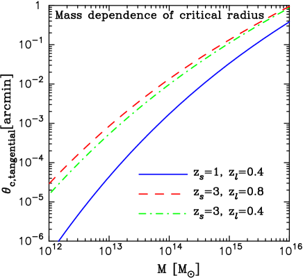
Figure 1: The tangential critical radius of NFW profile against halo masses. The solid and dashed curves are the results for lensing halos at redshifts of $z_{l}=0.4$ and $0.8$ for source redshifts of $z_{s}=1$ and $z_{s}=3$, respectively. Even if we consider a lower lens redshift, the result does not largely change, as shown by the dot-dashed curve.

Any lensing NFW halo inevitably provides finite critical radius, if we have an ideal angular resolution. This is because the convergence $\kappa_{M}$ varies from zero to infinity with changing radius from $\theta_{\rm 180}$ to $0$, while the shear remains finite over the range (see Figure 2 in TJ03c). Figure 1 plots the tangential critical radius for a lensing NFW halo against the mass. Note that an NFW profile produces two critical radii – an outer curve causes a tangentially deformed image around it, while the inner one causes a radially deformed image. The solid and dashed curves are the results for halos at redshifts $z_{l}=0.4$ and $0.8$ for source redshifts of $z_{s}=1.0$ and $3.0$, respectively. One can see that the critical radius has a strong dependence on halo masses and is larger for $z_{s}=3$ than for $z_{s}=1$ due to the greater lensing efficiency. These critical curves do not largely change even if we consider a lower lens redshift than the peak redshift, as shown by the dot-dashed curve. Even massive halos with $M\sim 10^{15}M_{\odot}$ provide the critical radii of $\lower 2.15277pt\hbox{$\;\buildrel<\over{\sim}\;$}0.\!\!^{\prime}1$. The scale is below relevant angular scales for the magnification statistics of our interest. However, this does not mean that the non-linear magnification correction to the correlation function appears only on scales $\lower 2.15277pt\hbox{$\;\buildrel<\over{\sim}\;$}1^{\prime}$. Rather, modest non-linear magnifications ($\mu\lower 2.15277pt\hbox{$\;\buildrel>\over{\sim}\;$}2$) lead to the strong impact, since such magnifications have larger cross section, as will be shown in detail.

3.3 Real-space halo model approach

In the following, we construct the halo model method to compute the magnification induced correlation function. First, we simply consider the 2PCF defined as

$$\xi_{\mu}(\theta)\equiv\left\langle{[\mu(\mbox{{\it\boldmath$\phi$}})-1][\mu(\mbox{{\it\boldmath$\phi$}}+\mbox{{\it\boldmath$\theta$}})-1]}\right\rangle,$$ (14)

where $\mu-1$ is the magnification fluctuation field. This 2PCF is observable from size fluctuations of distant galaxy images, as discussed in §2.2.

From a picture of the halo model, $\xi_{\mu}(\theta)$ can be expressed as a sum of correlations between the magnifications fields within a single halo (1-halo term) and between two different halos (2-halo term):

$$\xi_{\mu}(\theta)=\xi_{\mu}^{1h}(\theta)+\xi_{\mu}^{2h}(\theta).$$ (15)

It is straightforward to extend the real-space halo model developed in TJ03a,b,c to compute the 1-halo term contribution, which has dominant contribution on small non-linear scales (see equations (19) and (20) in TJ03c):

$$\xi_{\mu}^{1h}(\theta) = \int^{\chi_{H}}_{0}\!\!d\chi\frac{d^{2}V}{d\chi d\Omega}\int\!\!dM~{}n(M)$$ (16)

$$\times\int^{\infty}_{0}\!\!d\phi\int^{2\pi}_{0}\!\!d\varphi~{}\phi\left[\mu_{M}(\phi)-1\right]\left[\mu_{M}(|\mbox{{\it\boldmath$\phi$}}+\mbox{{\it\boldmath$\theta$}}|)-1\right],$$

where we have introduced the polar coordinate $d^{2}\mbox{{\it\boldmath$\phi$}}=\phi d\phi d\varphi$, $d^{2}V/d\chi d\Omega=d_{A}^{2}(\chi)$ for a flat universe and we can set the separation vector $\theta$ to be along the first axis from statistical symmetry, thereby $|\mbox{{\it\boldmath$\phi$}}+\mbox{{\it\boldmath$\theta$}}|=(\phi^{2}+\theta^{2}+2\phi\theta\cos\varphi)^{1/2}$. We have assumed a uniform distribution of sources on the sky and ignored a probability of multiple images and an increase or decrease in sampling of the images due to the lensing itself (which is a higher order correction and can be safely neglected as shown in Hamana 2001). The equation above implies that the 1-halo term contribution is given by summing lensing contributions due to halos along the line-of-sight weighted with the halo number density on the light cone. Note that the integration range of $d^{2}\mbox{{\it\boldmath$\phi$}}$ is taken as the infinite area, taking into account the non-local property of the shear field that is non-vanishing at radius outside the halo boundary. In practice, setting the upper bound of $\int\!\!d\phi$ to be three times the projected radius $\theta_{180}$ gives the same result, to within a few percents. The validity of the real-space halo model formulation was carefully investigated in TJ03b,c.

As discussed in §3.2 and shown in Figure 1, an NFW profile always provides finite critical curves, where the magnification formally becomes infinity. Therefore, to make the halo model prediction, we introduce a magnification cutoff $\mu_{\rm max}$ in the calculation – the integration range of $\int\!\!d^{2}\mbox{{\it\boldmath$\phi$}}$ is confined to the region satisfying the condition $\mu_{M}\leq\mu_{\rm max}$ for a given halo. This procedure is somehow similar to what is done in the measurement from ray-tracing simulations, where a masking of high magnification events is employed to avoid a significant statistical scatter (e.g., see Ménard et al. 2003; Barber & Taylor 2002). Thus the halo model allows for a fair comparison of the prediction with the simulation result. However, note that the procedure taken ignores the lensing projection effect for simplicity: exactly speaking, the magnification should be given by the lensing fields between source and observer, not by those of individual halo.

Similarly, based on the real-space halo model, the 2-halo term can be expressed as

$$\xi_{\mu}^{2h}(\theta) = \int_{0}^{\infty}\!\!d\chi~{}\frac{d^{2}V}{d\chi d\Omega}\int\!\!dM~{}n(M)\int\!\!dM^{\prime}~{}n(M^{\prime})$$

$$\times\int\!\!d^{2}\mbox{{\it\boldmath$\phi$}}\left[\mu_{M}(\phi)-1\right]\int\!\!d^{2}\mbox{{\it\boldmath$\phi^{\prime}$}}\left[\mu_{M^{\prime}}(\phi^{\prime})-1\right]$$

$$\times b(M)b(M^{\prime})\int\!\!\frac{ldl}{2\pi}P^{L}\!\left(k=\frac{l}{d_{A}};\chi\right)J_{0}(l|\mbox{{\it\boldmath$\theta$}}-\mbox{{\it\boldmath$\phi$}}-\mbox{{\it\boldmath$\phi$}}^{\prime}|),$$

where $J_{0}(x)$ is the zero-th order Bessel function and $P^{L}(k)$ is the linear mass power spectrum at epoch $\chi$ as given by $P^{L}(k;\chi)=D^{2}(\chi)P(k;t_{0})$. The term including $P^{L}(k)$ in the third line on the r.h.s denotes the angular two-point correlation function between different halos of masses $M$ and $M^{\prime}$, which is derived using Limber’s equation and the flat-sky approximation (e.g., Blandford et al. 1991; Miralda-Escude 1991; Kaiser 1992). We similarly introduce the maximum magnification cutoff in the 2-halo term calculation as in the 1-halo term. The equation above means that we have to perform an 8-dimensional integration to get the 2-halo term, which is computationally intractable. For this reason, we employ an approximated way to be valid when angular separation between the two halos taken is much greater than their angular virial radii. This leads to a simplified expression of the 2-halo term:

$$\xi_{\mu}^{2h}(\theta) \approx \int_{0}^{\infty}\!\!d\chi~{}\frac{d^{2}V}{d\chi d\Omega}$$ (18)

$$\times\left[\int\!\!dM~{}b(M)n(M)\int\!\!\phi d\phi~{}2\pi(\mu_{M}(\phi)-1)\right]^{2}$$

$$\times\int\!\!\frac{ldl}{2\pi}~{}P^{L}\!\left(k=\frac{l}{d_{A}(\chi)};\chi\right)J_{0}(l\theta).$$

This allows us to get the 2-halo term by a three-dimensional integration, because the integrations of the second and third lines on the r.h.s can be done separately before performing the $\chi$-integration. It is worth checking the consistency of the 2-halo term above with the limiting case $\xi_{\mu}\approx 4\xi_{\kappa}$, which is valid in the weak lensing limit $\mu\approx 1+2\kappa$ for $\kappa,\gamma\ll 1$. In this limit, the term contained in the second line on the r.h.s of equation (18) can be rewritten as

$$\int\!\!dM~{}b(M)n(M)\int\!\!d^{2}\mbox{{\it\boldmath$\phi$}}~{}(\mu_{M}(\phi)-1)$$ (19)

$$\approx\int\!\!dM~{}b(M)n(M)\int\!\!d^{2}\mbox{{\it\boldmath$\phi$}}~{}2\kappa_{M}(\phi)$$

$$=2W(\chi)d_{A}^{-2}(\chi)\int\!\!dM~{}b(M)n(M)\frac{M}{\bar{\rho}_{0}},$$

where the second equality is derived from equations (25) and (28) in TJ03b. Therefore, substituting this result into the 2-halo term (18) yields

$$\xi_{\mu}^{2h}(\theta) \approx 4\int_{0}^{\infty}\!\!d\chi~{}W^{2}(\chi)d_{A}^{-2}(\chi)$$ (20)

$$\times\left[\int\!\!dM~{}b(M)n(M)\frac{M}{\bar{\rho}_{0}}\right]^{2}$$

$$\times\int\!\!\frac{ldl}{2\pi}~{}P^{L}\!\left(k=\frac{l}{d_{A}(\chi)};\chi\right)J_{0}(l\theta)$$

$$= 4\xi_{\kappa}^{2h}(\theta).$$

The 2-halo term (18) is thus reduced to four times the 2-halo term of the convergence 2PCF in the weak lensing limit, as expected. However, the important point of the 2-halo term (18) is that it can correctly account for the contribution of non-linear magnifications ($\mu\lower 2.15277pt\hbox{$\;\buildrel>\over{\sim}\;$}2$) on large scales.

Replacing $P^{2h}(k)$ in equation (20) with a model of the non-linear mass power spectrum leads to the conventional method for predicting $4\xi_{\kappa}(\theta)$ as an estimator of $\xi_{\mu}(\theta)$, as employed in the literature (e.g., Dolag & Bartelmann 1997; Sanz et al. 1997; Jain et al. 2003).

4 Asymptotic behavior of magnification statistics for high magnifications

As stated in the preceding section, we need to introduce a maximum magnification cutoff in the model prediction to avoid the contribution from a formally emerged infinite magnification. In practice, strong lensing events of $\mu\gg 1$, which are identified by multiple images or largely deformed image, can be removed from the sample of the magnification statistics. However, without the clear signatures, it is hard to make the distinct selection and therefore modest magnification events ($\delta\mu\lower 2.15277pt\hbox{$\;\buildrel>\over{\sim}\;$}1$) are likely included in the sample for the blind analysis, because the magnification is not a direct observable. In the following, we clarify how the magnification statistics depend upon large magnification events ($\mu\gg 1$).

Meanwhile, we restrict our discussion to point-like sources for simplicity. High magnifications $(\mu\gg 1)$ arise from images in the vicinity of the critical curve that is caused by an intervening mass concentration, such as halos. For any finite lens mass distribution, the critical curve must form a closed non-self-intersecting loop. Based on the catastrophe theory, it was shown in Blandford & Narayan (1986; also see Chapter 6 in Schneider et al. 1992) that the magnification of an image at a perpendicular distance $\Delta\theta$ from the (fold) critical curve scales asymptotically as

$$\mu\propto\frac{1}{\Delta\theta}.$$ (21)

This argument holds independently of details of the lensing mass distribution, although the proportional coefficient does depend on the mass distribution.

To keep generality of our discussion, let us consider a correlation function between the magnification field and some cosmic fields expressed as

$$\xi(\theta;p)=\langle{[\mu(\mbox{{\it\boldmath$\theta$}}_{1})]^{p}f(\mbox{{\it\boldmath$\theta$}}_{2})}\rangle_{|\mbox{{\it\boldmath$\theta$}}_{1}-\mbox{{\it\boldmath$\theta$}}_{2}|=\theta},$$ (22)

where $p$ is an arbitrary number. The field $f$ is allowed to be constituted from any cosmic fields which are correlated with the magnification field. Therefore, the following argument holds for high-order moments beyond the two-point correlations if one takes products of the cosmic fields for $f$, e.g. $f=\delta(\mbox{{\it\boldmath$\theta$}}_{2})\delta(\mbox{{\it\boldmath$\theta$}}_{3})$.

Suppose that an intervening halo provides the critical curve in the lens plane for a given source redshift, as this is the case for an NFW halo (see Figure 1). Then, let us consider how high magnifications in the vicinity of this critical curve contribute to the magnification statistics. By introducing an upper bound on the magnification fields as $\mu\leq\mu_{\rm max}$, we can address how the magnification statistics depend on the cutoff $\mu_{\rm max}$ and what is the asymptotic behavior for the limiting case $\mu_{\rm max}\rightarrow\infty$. From equation (21), the cutoff $\mu_{\rm max}$ corresponds to a lower limit on the perpendicular distance from the critical curve, say $\Delta\theta\geq\epsilon$ ($\epsilon\rightarrow 0$ corresponds to $\mu_{\rm max}\rightarrow\infty$). As can be seen from equations (16) and (18), a picture of the halo model leads us to compute the high magnification contribution to the magnification-induced correlation like equation (22) by the integration

$$\xi(\theta;p,\mu_{\rm max})\sim\int_{\partial S_{c},\mu\leq\mu_{\rm max}}\!d^{2}\mbox{{\it\boldmath$s$}}~{}\frac{1}{|\Delta s|^{p}}f(|\mbox{{\it\boldmath$s$}}+\mbox{{\it\boldmath$\theta$}}|),$$ (23)

where $\Delta s$ is the perpendicular distance from the critical curve and the integration range is confined to the area $\partial S_{c}$ subject to the condition $\mu\leq\mu_{\rm max}$. The integration (23) results in one-dimensional integration for high magnifications around the critical curve, in analogy with equation (5.16) in Blandford & Narayan (1986) to derive the asymptotic, integral cross section for the strong lensing events that produce multiple images. Hence, the leading order contribution of $\mu_{\rm max}$ can be expressed as

$$\xi(\theta;p,\mu_{\rm max}) \sim \left\{\begin{array}[]{ll}1/\mu_{\rm max}^{1-p},&p<1\\ \ln(\mu_{\rm max}),&p=1\\ \mu_{\rm max}^{p-1},&p>1.\end{array}\right.$$ (27)

where we have assumed that variation in the field $f$ does not largely change for the relevant integration range. The equation above leads to an intriguing consequence: the amplitude of the magnification correlation is finite for $p<1$ for the limiting case $\mu_{\rm max}\rightarrow\infty$, while it diverges for $p\geq 1$. Thus, the statistics with $p<1$ is practically advantageous in that it is insensitive to the uncertainty of which magnification cutoff should be imposed for a given sample. Furthermore, the asymptotic behavior does not explicitly depend on the separation angle $\theta$ and therefore it holds even for large $\theta$. This means that the divergence $\xi\rightarrow\infty$ for $p\geq 1$ formally occurs even on degree scales, which is opposed to a naive expectation that the weak lensing approximation is safely valid on these scales. It is also worth stressing that this behavior is expected to hold for any lensing mass distribution once the critical curve appears, although the proportionality coefficient of $\xi$ should depend on details of the mass distribution. These will be quantitatively tested by the halo model prediction as well as by the ray-tracing simulation.

In reality, a finite source size imposes a maximum cutoff on the observed magnification and thus the infinite magnification does not happen, even if a source sits on the caustic curve in the source plane (see Chapters 6 and 7 in Schneider et al. 1992; Peacock 1982; Blandford & Narayan 1996). For example, if the source is a circular disk with radius $r_{S}$ and uniform surface brightness, the maximum magnification is given by $\mu_{\rm max}\propto 1/\sqrt{r_{S}}$. Therefore, to develop an accurate model prediction requires a knowledge of unlensed source properties such as the size and the surface brightness distribution in addition to modeling the lensing mass distribution. In particular, this could be crucial if one considers the magnification statistics (22) with $p\geq 1$, since it is sensitive to large magnification events.

5 Results

5.1 Ray-tracing simulations

To test the analytic method developed in §3, we employ the ray-tracing simulations. We will use the simulation for the current concordance $\Lambda$CDM model with $\Omega_{\rm m0}=0.3$, $\Omega_{\lambda 0}=0.7$, $\Omega_{\rm b0}=0.04$, $h=0.7$ and $\sigma_{8}=0.9$ (Ménard et al. 2003; Hamana et al. in preparation; TJ03c). The $N$-body simulations were carried out by the Virgo Consortium (see also Yoshida, Sheth & Diaferio 2001), and were run using the particle-particle/particle-mesh (P³M) code with a force softening length of $l_{\rm soft}\sim 30h^{-1}$kpc. The initial matter power spectrum was computed using CMBFAST (Seljak & Zaldarriaga 1996). For the analytic model, we approximate the initial condition to use the CDM transfer function given by Bardeen et al. (1986) with the shape parameter in Sugiyama (1995) for simplicity. The $N$-body simulation employs $512^{3}$ CDM particles in a cubic box of $479h^{-1}$Mpc on a side, and the particle mass of the simulation is $m_{\rm part}=6.8\times 10^{10}h^{-1}M_{\odot}$.

The multiple-lens plane algorithm to simulate the lensing maps from the $N$-body simulations is detailed in Jain et al. (2000) and Hamana & Mellier (2001). We will use the output data for source redshifts of $z_{s}=1$ and 3 for the following analysis. The simulated map is given on $1024^{2}$ grids of a size of $\theta_{\rm grid}=0.\!\!^{\prime}2$; the area is $\Omega_{s}=11.7$ degree². The angular resolution that is unlikely affected by the discreteness of the $N$-body simulation is around $1^{\prime}$ (Ménard et al. 2003; TJ03c).

5.2 Probability distribution function of the magnification: the angular resolution of the simulations

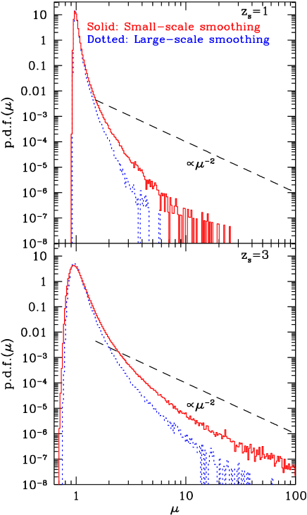
Figure 2: The probability density function (PDF) of the magnification measured from the ray-tracing simulations for $z_{s}=1$ and $3$. To clarify the angular resolution, we show the two results of using different smoothing scales, which were used to avoid the artificial discrete effect of the $N$-body simulations. The comparison manifests that high magnification events are sensitive to smaller structures that are relevant for the smoothing. The dashed line shows an asymptotic behavior of the PDF for high magnification events, ${\rm PDF}\propto\mu^{-2}$, as theoretically expected (see text in more detail).

Universal properties of the critical curve, as demonstrated in §4, lead to an asymptotic behavior of the probability distribution function (PDF) of large magnification events, irrespective of details of the lensing mass distribution: ${\rm PDF}(\mu)\propto\mu^{-2}$ (Peacock 1982; Vierti & Ostriker 1983; Blandford & Narayan 1986; Schneider 1987; Hamana, Martel & Futamase 2000, and also see Chapters 6, 11 and 12 of Schneider et al. 1992). Note that the PDF is defined in the image plane, while the PDF becomes $\mu^{-3}$ if one defines it from the sample of sources in the source plane. We use this property to investigate the angular resolution of the ray-tracing simulation.

Figures 2 shows the magnification PDF measured in the simulations for source redshifts of $z_{s}=1$ and $3$, respectively. To compute the PDF, we accumulate the counts in a given bin of $\mu$ from 36 realizations and then normalize the PDF amplitude to satisfy $\int\!\!d\mu~{}{\rm PDF}(\mu)=1$ over the range of $\mu$ measured. The PDF has a skewed distribution: most events lie in demagnification of $\mu<1$ and rare events have high magnifications with $\mu\gg 1$ having a long tail. These reflect an asymmetric mass distribution in the large-scale structure as expected from the CDM scenario – the underdense region can be seen preferentially in the void region with a typical size $\sim 10$Mpc, while the highly non-linear structures appear in dark matter halos on scales $\;\buildrel<\over{\sim}\;$Mpc. As can be seen, the simulation of $z_{s}=3$ displays more pronounced evidence of asymptotic dependence ${\rm PDF}(\mu)\propto\mu^{-2}$ for high magnifications ($\mu\lower 2.15277pt\hbox{$\;\buildrel>\over{\sim}\;$}10$) than the result for $z_{s}=1$.

To more explicitly clarify the resolution issue of the simulations, we show the two results of the different smoothing scales that were used in making the projected density field to suppress the discreteness effect of the $N$-body simulations (see Ménard et al. 2003 and Hamana et al. 2003 for more details). They are named as ‘small-scale smoothing’ (solid curve) and ‘large-scale smoothing’ (dotted curve), respectively. The former is expected to have the angular resolution around $1^{\prime}$ as discussed in Ménard et al. (2003) and in TJ03c, while the latter employs a smoothing scale two times larger than the former. The effect of the large-scale smoothing is that it more smoothes out smaller scale structures of the mass distribution that are resolved by the small-scale smoothing simulation. The comparison manifests that occurrence of high magnification events ($\mu>1$) is very sensitive to the small-scale structures. For this reason, we will employ the small-smoothing simulation in the following, since our interest is to clarify the non-linear magnification effect on the magnification statistics. This result also implies that simulations with higher resolution could further alter the PDF shape especially at high magnification tail.

5.3 The two-point correlation function of lensing magnification

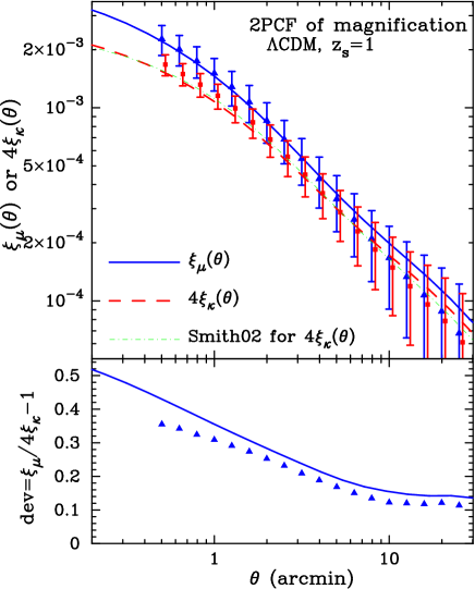
Figure 3: The two-point correlation function of the magnification field against the separation angle for the $\Lambda$CDM model and source redshift $z_{s}=1$. The solid curve shows the halo model prediction, while the triangle symbol is the simulation result. In most part of this paper, the maximum magnification cutoff $\mu_{\rm max}=8$ is employed (see text for the details). The error bar denotes the sample variance for a simulated area of $11.7$ degree². For comparison, the weak lensing predictions, leading to $\xi_{\mu}\approx 4\langle{\kappa\kappa}\rangle$, are shown by the halo model (dashed curve), the simulation (square symbol) and the fitting formula of Smith et al. (2003; dot-dashed curve). Note that the simulation result is slightly shifted in the horizontal direction for illustrative purpose. The lower panel explicitly plots the contribution of non-linear magnifications, $\xi_{\mu}/4\xi_{\kappa}-1$, for the halo model prediction and the simulation result.

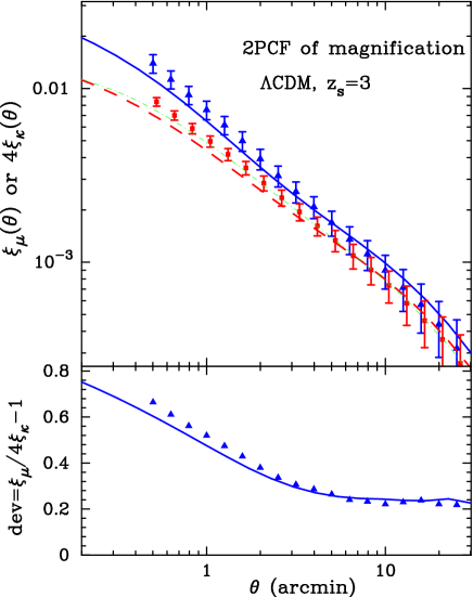
Figure 4: As in the previous figure, but for $z_{s}=3$. For higher source redshifts, the non-linear magnification effect becomes more significant as expected.

We now turn to investigation of the magnification 2PCF, $\xi_{\mu}\equiv\langle{\delta\mu\cdot\delta\mu}\rangle$, as it is possible to observe from size fluctuations on distant galaxy images (see §2.2). Figure 3 shows the comparison of the halo model prediction (solid curve) with the measurement from simulations (triangle symbol) for source redshift $z_{s}=1$. Note that the error bar in each bin denotes the sample variance for a simulated area of $11.7$ degree², which is computed from $36$ realizations, and the errors in neighboring bins are highly correlated. In this and following results, we mainly employ the maximum magnification cutoff $\mu_{\rm max}=8$ in the halo model prediction as well as in the simulation result. If we ignore the shear contribution to the magnification (1), this cutoff corresponds to $\mu\approx 1+2\kappa=2.3$ for the weak lensing approximation. The cutoff value is chosen so that strong lensing events are removed from the analysis, because such events likely have greater magnification $\mu\lower 2.15277pt\hbox{$\;\buildrel>\over{\sim}\;$}10$ (private communication with M. Oguri). Figure 2 shows that this cutoff leads us to exclude the events in a high magnification tail of the PDF.

Figure 3 shows that the halo model prediction well matches the simulation result. The 1-halo term provides dominant contribution to the total power on small scales $\lower 2.15277pt\hbox{$\;\buildrel<\over{\sim}\;$}3^{\prime}$, while the 2-halo term eventually captures the larger scale signal (see Figure A1 of TJ03c). It is worth noting that the shear field in $\mu$ (see equation (1)) contributes to the 2PCF amplitude by $\sim 10\%$ over the scales considered. To make clear the importance of the non-linear magnification contribution ($\delta\mu\lower 2.15277pt\hbox{$\;\buildrel>\over{\sim}\;$}1$), the dashed curve and the square symbol are the halo model prediction and the simulation result for the weak lensing approximation $\xi_{\mu}\approx 4\langle{\kappa\kappa}\rangle=4\xi_{\kappa}$. For this case, $4\xi_{\kappa}$ can be also computed from the fitting formula of the non-linear mass power spectrum recently proposed by Smith et al. (2003; hereafter Smith03), which demonstrates another test of the accuracy of the halo model as well as of the simulation.

The lower panel explicitly plots the relative difference, $\xi_{\mu}/4\xi_{\kappa}-1$. The simulation result is computed from the mean values of $\xi_{\mu}$ and $4\xi_{\kappa}$, and we do not plot the large error bar for illustrative purpose. The correction of the non-linear magnification amounts to $\lower 2.15277pt\hbox{$\;\buildrel>\over{\sim}\;$}30\%$ at $\theta\lower 2.15277pt\hbox{$\;\buildrel<\over{\sim}\;$}2^{\prime}$, and the non-negligible contribution of $\sim 10\%$ still remains even on large scales $\lower 2.15277pt\hbox{$\;\buildrel>\over{\sim}\;$}10^{\prime}$. Our model of the 2-halo term (18) correctly captures the non-linear effect seen in the simulation on the large scales. This large-scale correction is somewhat surprising, since it is naively expected that the weak lensing approximation is valid at these scales. Ménard et al. (2003) also showed that the non-linear correction on the large scales can be fairly explained taking into account the higher-order terms $O(\kappa^{2})$ in the Taylor expansion of $\mu$, though the method ceases to be accurate on small scales $\lower 2.15277pt\hbox{$\;\buildrel<\over{\sim}\;$}5^{\prime}$. One advantage of the halo model is that it allows us to explicitly introduce the maximum magnification cutoff in the calculation, which allows a fair comparison with the simulation and probably with the actual observation. In other words, the results shown depend upon the cutoff value employed. If we use the cutoff values of $\mu_{\rm max}=2$ and $100$, the deviation, $\xi_{\mu}/4\xi_{\kappa}-1$, becomes $\sim 20\%$ and $\sim 40\%$ at $\theta=1^{\prime}$, respectively (also see Figure 5).

Figure 4 shows the result for $z_{s}=3$, as in the previous figure. It is clear that the non-linear magnification contribution leads to significant enhancement in the amplitude of the magnification correlation relative to the weak lensing prediction. The enhancement is $\lower 2.15277pt\hbox{$\;\buildrel>\over{\sim}\;$}40\%$ at $\theta\lower 2.15277pt\hbox{$\;\buildrel<\over{\sim}\;$}2^{\prime}$. The comparison with the previous figure manifests that sources at higher redshifts are more affected by the non-linear magnification, as the sources have more chance to encounter intervening halos. It is worth noting that, if we do not apply any masking of high magnification events in the simulation, the statistical error in each bin becomes very large, which indicates the presence of events with $\mu\gg 1$ in some realizations as shown in Figure 2.

5.4 A quantitative test of the asymptotic behavior of the magnification statistics

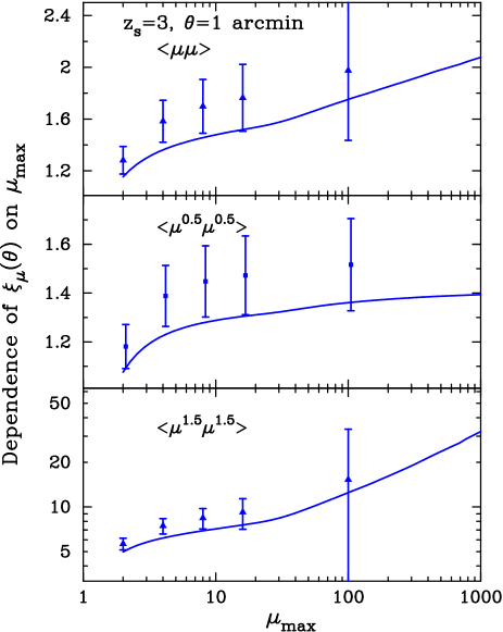
Figure 5: Dependences of the magnification 2PCF amplitude on the maximum magnification cutoff used in the evaluations. For the magnification correlation parameterized as $\langle{\delta\mu^{p}\cdot\delta\mu^{p}}\rangle$, the three panels show the results for $p=1$, $0.5$ and $1.5$, respectively. The source redshift $z_{s}=3$ and the separation angle $\theta=1^{\prime}$ are considered. All the curves are normalized by the predictions derived from the weak lensing approximation $(\mu\approx 1+2\kappa)$. As discussed in §4, it is expected that the 2PCF amplitude diverges for $p\geq 1$ for the limiting case $\mu_{\rm max}\rightarrow\infty$, while it remains finite for $p<1$ (see equation (27)). This is verified by the halo model as well as by the simulation.

In what follows we quantitatively test the asymptotic dependence of the magnification statistics on large magnifications ($\mu\gg 1$), as derived in §4. For this purpose, we consider three cases of $p=0.5$, $1$ and $1.5$ for the magnification 2PCF parameterized as $\xi=\langle{\delta\!\mu^{p}\cdot\delta\!\mu^{p}}\rangle$, with source redshift $z_{s}=3$. Figure 5 shows how the 2PCF amplitude depends on the magnification cutoff $\mu_{\rm max}$ used in the halo model predictions and the simulation result. The separation angle of $\theta=1^{\prime}$ is considered and the curves are normalized by the predictions from the weak lensing approximation. The scale $\theta=1^{\prime}$ is chosen based on the fact that the scale is in the non-linear regime and unlikely affected by the angular resolution of the simulation (TJ03c). First, one can see that even the most conservative choice of $\mu_{\rm max}=2$ leads to decent difference between the correct treatment and the weak lensing approximation. The consequence derived in §4 is that the 2PCF amplitudes for $p=0.5$, $1.0$ and $1.5$ have the dependences on $\mu_{\rm max}$ given as $\xi\propto\mu_{\rm max}^{-0.5}$, $\ln(\mu_{\rm max})$ and $\mu_{\rm max}^{0.5}$ for $\mu_{\rm max}\gg 1$, respectively. It is obvious that this consequence is verified by the halo model prediction as well as by the simulation result for $\mu_{\rm max}\lower 2.15277pt\hbox{$\;\buildrel>\over{\sim}\;$}10$. Although the halo model results for $\alpha=1.0$ and $1.5$ display a bend at $\mu_{\rm max}\approx 30$, we found that this is due to high magnifications between the radial and tangential critical curves in NFW halos. Most importantly, the 2PCF amplitude for $p=0.5$ has a well converged value for $\mu_{\rm max}\lower 2.15277pt\hbox{$\;\buildrel>\over{\sim}\;$}5$: the amplitude changes by less than $10\%$ over $\mu_{\rm max}=[10,1000]$. Therefore, the statistics with $p<1$ have a practically great advantage because it is little affected by the uncertainty in specifying the maximum magnification cutoff in the analysis.

Finally, we note that the results shown above are unchanged even if we consider the cross-correlation $\langle{\delta\!\mu^{p}\cdot\delta^{2D}}\rangle$, where $\delta^{2D}$ is the projected density fluctuation field (e.g., see equation (28)), because the asymptotic behavior is determined by the power of $\mu$ entering into the general correlation function $\langle{\mu^{p}f}\rangle$, as derived in §4.

5.5 Application to QSO-galaxy cross correlation

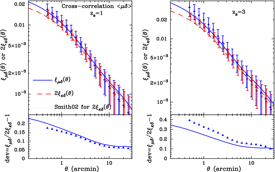
Figure 6: The cross correlation function between the magnification field and the projected density fluctuation field for $z_{s}=1$ (left panel) and 3 (right panel), as in Figure 3. To get the projected density field, we assume the redshift selection function given by equation (29).

In this subsection, we consider an application of the halo model to the QSO-galaxy cross correlation. The angular fluctuation field of galaxies on the sky is a projection of the 3D galaxy fluctuation field $\delta^{g}$ along the line-of-sight, weighted with the redshift selection function $f_{g}(z)$ of the galaxy sample:

$$\delta n^{g}(\bar{\theta})=\int^{\infty}_{0}\!\!dz~{}f_{g}(z)~{}\delta^{g}(d_{A}(z)\mbox{{\it\boldmath$\theta$}},z),$$ (28)

where $f_{g}(z)$ is normalized as $\int^{\infty}_{0}\!dzf_{g}(z)=1$. Throughout this paper, we employ

$$f_{g}(z)dz=\frac{\beta z^{2}}{z_{0}^{3}\Gamma(3/\beta)}\exp\left[-\left(\frac{z}{z_{0}}\right)^{\beta}\right]dz,$$ (29)

with $\beta=1.5$ and $z_{0}=0.3$. This model leads to the mean redshift as $z_{\rm mean}=\int\!\!dz~{}zf_{g}(z)=0.45$ and roughly reproduces the actual distribution of galaxies in the redshift galaxy catalog (e.g., Dodelson et al. 2002).

However, the galaxy fluctuation field $\delta^{g}$ is not straightforward to model, since the galaxy formation is affected by complex astrophysical processes in addition to the gravitational effect. Recently, Jain et al. (2003) developed a sophisticated description of the magnification correlations based on the halo model as well as the semi-analytic galaxy formation model. In particular, it was shown that it is crucial to account for a realistic model to describe how galaxies populate their parent halo, the so-called halo occupation number, to make the accurate model predictions on arcminute angular scales. The halo occupation number strongly depends on types of galaxies such red or blue galaxies. We here address how the non-linear magnification further modifies the model prediction.

Before going to this study, we consider the cross-correlation between the magnification field and the dark matter distribution, which corresponds to an unrealistic case that the galaxy distribution exactly traces the underlying mass distribution; $\delta_{\rm g}=\delta$. This investigation is aimed at clarifying how the non-linear magnification effect remains after inclusion of a realistic model of the galaxy clustering, from the comparison of the results with and without the galaxy bias model. In addition, in this case we can compare the model prediction with the simulation result that is computed from the same $N$-body simulation we have used. Extending the method presented in §3 leads to the 1-halo term contribution to the cross-correlation:

$$\xi^{1h}_{\mu\delta}(\theta) = \int^{\chi_{H}}_{0}\!\!d\chi\frac{d^{2}V}{d\chi d\Omega}f_{g}(z)\frac{dz}{d\chi}\int\!\!dM~{}n(M)\frac{M}{\bar{\rho}_{0}}$$ (30)

$$\times\int^{\infty}_{0}\!\!d\phi\int^{2\pi}_{0}\!\!d\varphi~{}\phi\left[\mu_{M}^{2.5s-1}(|\mbox{{\it\boldmath$\phi$}}+\mbox{{\it\boldmath$\theta$}}|)-1\right]\Sigma_{M}(\phi),$$

where $\Sigma_{M}(x)$ is the normalized projected density of the NFW profile given by equation (26) in TJ03b. Similarly, one can derive the 2-halo term of $\xi_{\mu\delta}$, as done by equation (18).

In Figure 6 we shows the results for source redshifts of $z_{s}=1$ (left panel) and $3$ (right panel), as in Figures 3 and 4. Note that both the results employ the same redshift selection function (29) to obtain the projected density field. We simply assumed a special case of $s=4/5$ for the magnitude slope for the unlensed QSO number count. From the comparison with Figures 3 and 4, it is clear that the non-linear magnification contribution is weakened, due to the single power of $\mu$ entering into the two-point correlation compared to the magnification 2PCF. Nevertheless, it should be stressed that the non-linear correction has significant contributions of $\lower 2.15277pt\hbox{$\;\buildrel>\over{\sim}\;$}15\%$ and $\lower 2.15277pt\hbox{$\;\buildrel>\over{\sim}\;$}25\%$ at $\theta\lower 2.15277pt\hbox{$\;\buildrel<\over{\sim}\;$}1^{\prime}$ for $z_{s}=1$ and 3, respectively.

Next, we consider a model of the QSO-galaxy correlation that takes into account both the galaxy bias and the non-linear magnification effect. To do this, we use the halo occupation number $\langle{N_{\rm g}(M)}\rangle$ to describe how many galaxies populate their parent halo of a given mass $M$, in an average sense (e.g., Seljak 2000; Guzik & Seljak 2002; Jain et al. 2003; TJ03b; Cooray & Sheth 2002). Simply replacing $M/\bar{\rho}_{0}$ in equation (30) with $\langle{N_{\rm g}(M)}\rangle/\bar{n}_{\rm gal}$ leads to the 1-halo term of the QSO-galaxy cross correlation:

$$\xi^{1h}_{\mu{\rm g}}(\theta) = \int^{\chi_{H}}_{0}\!\!d\chi\frac{d^{2}V}{d\chi d\Omega}f_{g}(z)\frac{dz}{d\chi}\int\!\!dM~{}n(M)\frac{\langle{N_{g}(M)}\rangle}{\bar{n}_{\rm gal}}$$ (31)

$$\times\int^{\infty}_{0}\!\!d\phi\int^{2\pi}_{0}\!\!d\varphi~{}\phi\left[\mu_{M}^{2.5s-1}(\phi)-1\right]\Sigma_{M}(|\mbox{{\it\boldmath$\phi$}}+\mbox{{\it\boldmath$\theta$}}|),$$

where $\bar{n}_{\rm gal}$ is the average number density at epoch $z$ defined as $\bar{n}_{\rm gal}=\int\!\!dM~{}n(M)\langle{N_{\rm g}(M)}\rangle$. The cross-correlation thus depends on the first moment of $\langle{N_{\rm g}(M)}\rangle$ . Note that, on the other hand, the two-point correlation of galaxies depends on the second moment, and it contains somehow uncertainty in modeling the sub-Poissonian process in the regime of $\langle{N_{\rm g}(M)}\rangle<1$.

As stressed in Guzik & Seljak (2002) and Jain et al. (2003), it is probably accurate to assume that one of the $\langle{N_{\rm g}}\rangle$ galaxies in a halo sits at the halo center and this has decent impact on the model predictions. On the other hand, we assume that the other $(\langle{N_{\rm g}}\rangle-1)$ galaxies follow the dark matter distribution within the halo. Following the method of Jain et al. (2003), the part of the integrand function in the 1-halo term (31) can be expressed as

$$\langle{N_{g}(M)}\rangle\int^{\infty}_{0}\!\!d\phi\int^{2\pi}_{0}\!\!d\varphi~{}\phi\left[\mu_{M}^{2.5s-1}(\phi)-1\right]\Sigma_{M}(|\mbox{{\it\boldmath$\phi$}}+\mbox{{\it\boldmath$\theta$}}|)$$ (32)

$$= \chi^{-2}\left[\mu_{M}^{2.5s-1}(\theta)-1\right]$$

$$+\int^{\infty}_{0}\!\!d\phi\int^{2\pi}_{0}\!\!d\varphi~{}\phi\left[\mu_{M}^{2.5s-1}(\phi)-1\right]\Sigma_{M}(|\mbox{{\it\boldmath$\phi$}}+\mbox{{\it\boldmath$\theta$}}|)$$

$$\times\left[\langle{N_{g}(M)}\rangle-1\right],$$

for $\langle{N_{g}(M)}\rangle\geq 1$ and

$$= \left[\mu_{M}^{2.5s-1}(\theta)-1\right]\langle{N_{g}(M)}\rangle,$$ (33)

for $\langle{N_{g}(M)}\rangle<1$. Substituting these equations into equation (31) leads to the halo model prediction for the QSO-galaxy cross-correlation.

To complete the model prediction, we need an adequately accurate model of the halo occupation number $\langle{N_{\rm g}(M)}\rangle$. We employed the model in Jain et al. (2003), which was derived from the GIF $N$-body simulations, coupled to a semi-analytic galaxy formation model (Kauffmann et al. 1999). The simulation result of $\langle{N_{\rm g}(M)}\rangle$ is well fitted by the functional form,

$$\langle{N_{g}(M)}\rangle=\left(\frac{M}{M_{0}}\right)^{\alpha}+A\exp\left[-A_{0}\left(\log_{10}(M)-M_{B}\right)^{2}\right].$$ (34)

The parameter values are taken from Table 1 labeled as ‘$z=0.06$’ in Jain et al. (2003), which reproduces the measurements for total (blue plus red) galaxies at $z=0.06$ in the GIF simulations. In the following, we employ a lower mass cutoff of $M\geq 10^{11}~{}h^{-1}M_{\odot}$ and ignore the redshift evolution of $\langle{N_{\rm g}(M)}\rangle$ for simplicity. This model leads to the galaxy bias parameter $\bar{b}_{\rm gal}=(1/\bar{n}_{\rm gal})\int\!dMn(M)b(M)\langle{N_{\rm g}(M)}\rangle=1.2$ at $z=0$ in the large-scale limit, thus reflecting the fact that the modeled galaxies are biased objects relative to the dark matter distribution.

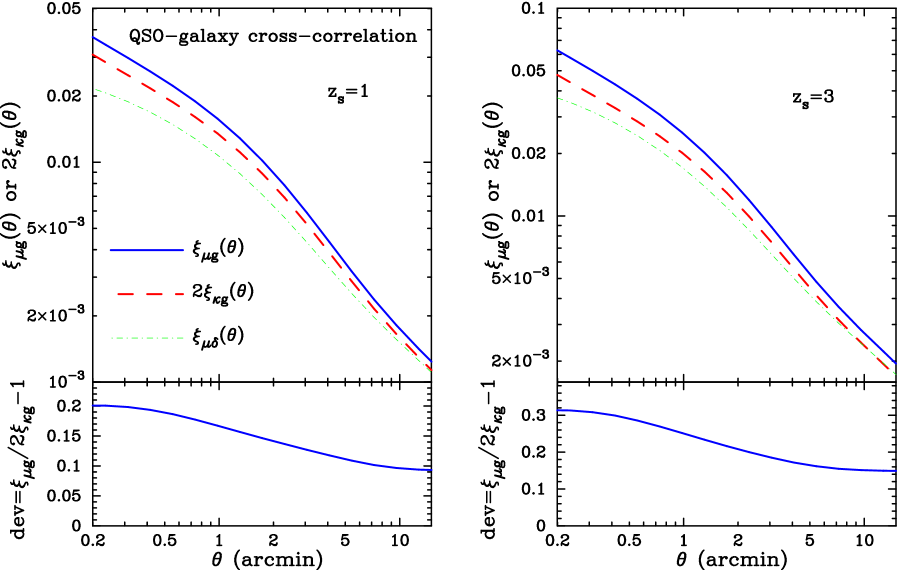
Figure 7: The halo model predictions for the angular cross-correlation between the magnification and the foreground galaxy distribution, where the galaxy clustering is modeled by the halo occupation number (34). For comparison, the dot-dashed curve is the result for the cross-correlation between the magnification and the projected dark matter distribution as shown in the previous figure. The non-linear magnification correction remains to enhance the cross-correlation amplitude relative to the weak lensing approximation, even if the realistic model of the galaxy clustering is included.

Figure 7 shows the model predictions for the QSO-galaxy cross-correlation, as in the previous figure. For comparison, the dot-dashed curve is the result for the cross-correlation between the magnification and the projected dark matter distribution in the previous figure. The comparison of the solid and dot-dashed curves manifests that the realistic model of galaxy bias largely modifies the cross-correlation, and the galaxy bias cannot be described by a simple linear bias on the small angular scales (Jain et al. 2003). It is also clear that the non-linear magnification correction is $10-25\%$ on arcminute scales. Therefore, this result implies that an inclusion of the non-linear effect will be necessary to make an unbiased interpretation of the precise measurement expected from forthcoming massive surveys such as the CFHT Legacy Survey and the SDSS.

5.6 Sensitivity of the magnification statistics to the halo profile properties

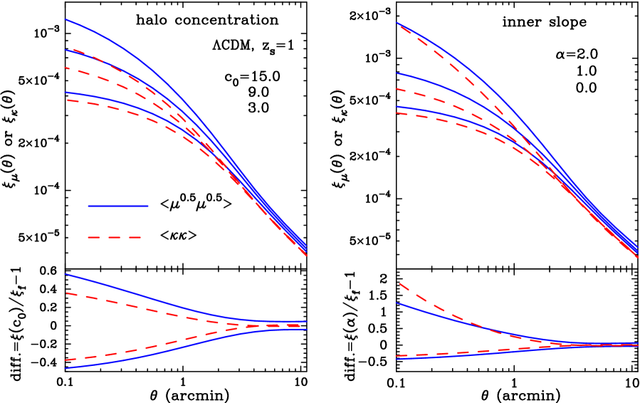
Figure 8: The dependences of the magnification 2PCF, $\langle{\delta\!\mu^{0.5}\cdot\delta\!\mu^{0.5}}\rangle$, on the halo profile parameters. The left panel shows the halo model predictions for the halo concentration parameter $c_{0}=3,9$ and $15$ (from bottom to top), while the right panel shows the results with $\alpha=0$, $1$ and $2$ for the inner slope parameter of the generalized NFW profile (see text for more details). For comparison, the dashed curves are the corresponding results for the convergence 2PCF. Note that the magnification 2PCF considered becomes equivalent to the convergence 2PCF in the weak lensing limit as $\delta\!\mu^{0.5}\approx\kappa$. The lower panel shows the difference relative to the result with our fiducial model of $\alpha=1$ and $c_{0}=9$.

As discussed above, one of the useful cosmological information extracted from the QSO-galaxy correlation measurement is information on the halo occupation number of galaxies, which in turn provides a clue to understanding of galaxy formation in connection to the dark matter halo properties (see Jain et al. 2003 for the details). We here demonstrate another possibility of the magnification statistics (especially measured via galaxy size fluctuations) to address questions: what can we learn from the measurements? How is this method complementary to the established cosmic shear that probes the correlations of the convergence or shear fields ($\kappa$ or $\gamma$)? To examine this, we focus on the non-linear relation between the magnification and the cosmic shear fields, as given by equation (1). The non-linear effect is more pronounced on smaller scales, as have so far been shown. Future massive surveys promise to measure the magnification statistics as well as the cosmic shear even on sub-arcminute scales (Jain 2002; TJ03c; Jain et al. 2003). Within a picture of the halo model, the sub-arcminute correlation function is quite sensitive to the halo profile properties (TJ03b,c) and the measurement can be potentially used to constrain the properties, if the systematics is well under control. Hence, we here investigate the dependence of the magnification 2PCF on the halo profile parameters, the halo concentration and the inner slope of the generalized NFW profile. These parameters are still uncertain observationally and theoretically and have information on the dark matter nature as well as properties of highly non-linear gravitational clustering on $\lower 2.15277pt\hbox{$\;\buildrel<\over{\sim}\;$}1$Mpc. Following TJ03c, we consider the parameterization given as $c(M,z)=r_{\rm vir}/r_{s}=c_{0}(M/M_{\ast})^{-0.13}$ and $\rho(r)\propto r^{-\alpha}(1+r/r_{s})^{-3+\alpha}$, respectively. Our fiducial model so far used is given by $(c_{0},\alpha)=(9.0,1.0)$. For cases $\alpha=0$, $1$ and $2$ we can derive analytic expressions for the convergence and shear profiles from which we can also compute the magnification profile (the expressions of the convergence fields are given in Appendix B in TJ03c). Note that in what follows we employ the virial boundary condition. The relevant angular scales are below the angular resolution of $N$-body simulations we have used.

The left panel of Figure 8 shows the halo model prediction for the magnification 2PCF with varying the halo concentration, while the right panel shows the results with varying $\alpha$. Here we consider $\langle{\delta\!\mu^{0.5}\cdot\delta\!\mu^{0.5}}\rangle$, because it is less sensitive to high magnification events ($\mu\gg 1$) and therefore observationally more robust (see Figure 5). In the weak lensing limit, the correlation can be approximated by the convergence 2PCF (dashed curves), which is measured by the cosmic shear measurement because $\delta\mu^{0.5}\approx\kappa$. Therefore, the difference between the solid and dashed curves reflects contribution from the non-linear magnifications $\delta\mu\lower 2.15277pt\hbox{$\;\buildrel>\over{\sim}\;$}1$. Halos with masses $M\geq 10^{13}M_{\odot}$ provide dominant contribution of $\lower 2.15277pt\hbox{$\;\buildrel>\over{\sim}\;$}80\%$ to the total power over a range of non-linear scales $0.\!\!^{\prime}1$-$3^{\prime}$ (e.g., see Figure 14 in TJ03c). One can see that the magnification 2PCF has stronger sensitivity to the halo concentration and depends on the inner slope in a different way from the convergence 2PCF. In TJ0c, it was pointed out that the cosmic shear measurement introduces a degeneracy in determining these halo profile parameters, even provided the accurate measurement (see Figures 16 and 17 in TJ03c). The results in Figure 8 thus indicate that a joint measurement of the magnification statistics and the cosmic shear can be used to improve the parameter determinations. Finally, one caution we make is that the magnification 2PCF for the profile with $\alpha=2$ is more amplified by an increase of the maximum magnification cutoff $\mu_{\rm max}$ than the other $\alpha$’s and thus is sensitive to the selection effect.

6 Discussions

In this paper, we have used the real-space halo approach to compute the magnification correlation function without employing the weak lensing approximation $\mu\approx 1+2\kappa+O(\kappa^{2})$. It has been shown that the correction due to the non-linear magnification ($\delta\mu\lower 2.15277pt\hbox{$\;\buildrel>\over{\sim}\;$}1$) leads to significant enhancement in the correlation amplitude relative to the weak lensing approximation (see Figures 3-7). The correction is more important as one considers the correlation function for sources at higher redshifts and on smaller angular scales, where the weak lensing approximation ceases to be accurate. Thus, accounting for the non-linear contribution in the theoretical model is needed to extract unbiased, cosmological information from the precise measurement expected from forthcoming and future surveys. The encouraging result shown is the halo model prediction remarkably well reproduces the simulation result over the angular scales we consider.

We also developed the model to predict the QSO-galaxy cross-correlation by incorporating the realistic model of the halo occupation number of galaxies into the halo model (see §5.5). The primary cosmological information provided from the measurement is constraints on the halo occupation number, as shown in Jain et al. (2003; also see Guzik & Seljak 2002). In particular, the QSO-galaxy correlation can be used to directly constrain the first moment of the halo occupation number, compared to the two-point correlation of galaxies that probes the second moment. Exploring the halo occupation is compelling in that it provides useful information on the galaxy formation and the merging history in connection with the dark matter halo properties. We showed that the non-linear magnification amplifies the cross-correlation amplitude by $10-25\%$ on arcminute scales. The method of this paper therefore provides the accurate model prediction that accounts for both the non-linear magnification correction and the realistic galaxy bias.

We found that the magnification statistics can be used to extract cosmological information complementary to that provided from the cosmic shear measurement. We have demonstrated that the joint measurement on angular scales $\lower 2.15277pt\hbox{$\;\buildrel<\over{\sim}\;$}3^{\prime}$ could be used to precisely constrain the halo profile properties (see Figure 8). This possibility would open a new direction in using the magnification statistics as a cosmological probe beyond determination of fundamental cosmological parameters (Bartelmann 1995; Bartelmann & Schneider 2001; Ménard & Bartelmann 2002; Ménard et al. 2003). Exploring the halo profile properties with gravitational lensing will be a direct test of the CDM scenario in the highly non-linear regime $\;\buildrel<\over{\sim}\;$Mpc, since alternative scenarios have been proposed in order to reconcile the possible conflicts between the CDM predictions and the observations on the small scales (e.g., Spergel & Steinhardt 2000).

In most results shown, we employed the maximum magnification cutoff $\mu_{\rm max}=8$ for the halo model predictions as well as for the simulation results, because the choice likely removes strong lensing events ($\mu\lower 2.15277pt\hbox{$\;\buildrel>\over{\sim}\;$}10$) from the analysis. Even if we employ the smaller value, the qualitative conclusions derived are not largely changed, as can be seen from Figure 5. Observationally, strong lensing event is easily removed from the sample of the magnification statistics, if it accompanies multiple images or largely deformed images. However, without the clear signature, it is relatively difficult to make a clear discrimination of the strong lensing, since the magnification is not a direct observable. One advantage of the halo model developed in this paper is that it allows a fair comparison with the measurement by employing the selection criteria in the measurement for the model prediction. Based on these considerations, we derived useful, general dependences of the magnification correlation amplitude on large magnifications $(\mu\gg 1)$, from the universal lensing properties in the vicinity of critical curves (see §4). The intriguing consequence is that, for a correlation function parameterized as $\langle{\mu^{p}f}\rangle$, the amplitude converges to be finite for $p<1$ and otherwise diverges $p\geq 1$ as the maximum magnification cutoff $\mu_{\rm max}\rightarrow\infty$, independent of details of the lensing mass distribution. This was quantitatively verified by the halo model prediction as well as by the simulations (see Figure 5). This result therefore implies that the magnification statistics with $p\leq 1$ are practically advantageous in that it is insensitive to the selection effect of the magnification cutoff $\mu_{\rm max}$. This is the case for the two-point correlation of size (not area) fluctuations of distant galaxy images and for the QSO-galaxy cross correlation, if the unlensed number counts of QSOs with a limiting magnitude have a slope of $s=d\ln N(m)/dm<4/5$.

One might imagine that the non-linear magnification contribution can be suppressed by clipping regions of cluster of galaxies from survey data in order to avoid the uncertainty in the model prediction and to apply the weak lensing approximation (e.g., see Barber & Taylor 2002). However, this likely adds an artificial selection effect in the analysis and causes a biased cosmological interpretation. In addition, the lensing projection makes it relatively difficult to correctly identify the cluster region from the reconstructed convergence map, unless accurate photo-$z$ information or follow-up observations are available (e.g., White et al. 2002). The approach of this paper allows us to treat data more objectively.

There are some effects we have so far ignored in the halo model calculation. Most important one is the asphericity of halo profile in a statistical sense. The aspherical effect could lead to substantial enhancement of the magnification correlation amplitude, since it is known that an area enclosed by the critical curve is largely increased by ellipticity of the lensing mass distribution, thus increasing the cross section of high magnifications to the correlation evaluation. For example, the number of strong lensing arcs due to clusters of galaxies is amplified by an order of magnitudes if one considers an elliptical lens model instead of an axially symmetric profile (e.g., Meneghetti et al. 2003; Oguri et al. 2003). For the same reason, substructures within a halo could have strong impact on the magnification correlation, as they naturally emerges in the CDM simulations. Hence, it is of great interest to investigate the effect on the magnification statistics with higher resolution simulations.

We are grateful to Bhuvnesh Jain for collaborative work, valuable discussions and a careful reading of the manuscript. T. H. would like to thank for his warm hospitality at University of Pennsylvania, where a part of this work was done. We also thank M. Bartelmann and M. Oguri for valuable discussions. T.H. also acknowledges supports from Japan Society for Promotion of Science (JSPS) Research Fellowships. Numerical computations presented in this paper were partly carried out at ADAC (the Astronomical Data Analysis Center) of the National Astronomical Observatory, Japan and at the computing centre of the Max-Planck Society in Garching. The $N$-body simulations used in this paper were carried out by the Virgo Supercomputing Consortium.

References

- [Barber & Taylor 2002] Barber, A. J., Taylor, A. N., 2002, astro-ph/0212378
- [Bardeen et al. 1986] Bardeen, J. M., Bond, J. R., Kaiser, N., Szalay, A. S., 1986, ApJ, 304, 15
- [Bartelmann 1995] Bartelmann, M., 1995, A&A, 298, 661
- [Bartelmann 1996] Bartelmann, M., 1996, A&A, 313, 697
- [Bartelmann & Narayan 1995] Bartelmann, M., Narayan, R., 1995, ApJ, 451, 60
- [Bartelmann & Schneider 2001] Bartelmann, M., Schneider, P., 2001, Phys. Rep. 340, 291
- [Benítez & Martínez-González 1997] Benítez, N., Martínez-González, E., 1997, ApJ, 477, 27
- [Benítez, Sanz & Martínez-González] Benítez, N., Sanz, J. L., Martínez-González, E., 2001, MNRAS, 320, 241
- [Blandford & Narayan 1986] Blandford, R. D., Narayan, R., 1986, ApJ, 310, 568
- [Blandford et al. 1991] Blandford, R. D., Saust, A. B., Brainerd, T. G., Villumsen, J. V., 1991, MNRAS, 251, 600
- [Broadhust, Taylor & Peacock 1995] Broadhurst, T. J., Taylor, A. N., Peacock, J. A., 1995, ApJ, 438, 49u
- [Bullock et al. 2001] Bullock, J. S., Kolatt, T. S., Sigad, Y., Somerville, R. S., Kravtsov, A. V., Klypin, A. A., Primack, J. R., Dekel, A., 2001, MNRAS, 321, 559
- [Cooray & Sheth 2002] Cooray, A., Sheth, R., 2002, Phys. Rep. , 372, 1
- [Dodelson et al. 2002] Dodelson, S., et al., 2002, ApJ, 572, 140
- [Dolag & Bartelmann 1997] Dolag, K., Bartelmann, M., 1997, MNRAS, 291, 446
- [Gaztañaga 2002] Gaztañaga, E., 2003, ApJ, 589, 82
- [Guzik] Guzik, J., Seljak, U., 2002, MNRAS, 335, 311
- [Hamana] Hamana, T., 2001, MNRAS, 326, 326
- [Hamana & Mellier 2001] Hamana, T., Mellier, Y., 2001, MNRAS, 327, 169
- [Hamana, Martel & Futamase 2000] Hamana, T., Martel, H., Futamase, T., 2000, ApJ, 529, 56
- [Hamana et al. 2002] Hamana, T., et al. 2002, astro-ph/0210450
- [Hattori et al. 1999] Hattori, M., Kneib, J.-P., Makino, N., 1999, Prog. Theor. Phys. Suppl., 133, 1
- [Hu & Kravtsov 2002] Hu, W., & Kravtsov, A., 2002, astro-ph/0203169
- [Jain 2002] Jain, B., 2002, ApJ, 580, L3
- [Jain, Scranton & Sheth 2003] Jain, B., Scranton, R., Sheth, R., 2003, astro-ph/0304203
- [Jain, Seljak & White 2000] Jain, B., Seljak, U., White, S. D. M., 2000, ApJ, 530, 547
- [] Jarvis, M., Bernstein, G., Jain, B., Fischer, P., Smith, D., Tyson, J. A., Wittman, D., 2003, AJ, 125, 1014
- [] Kauffmann, G., et al. 1999, MNRAS, 307, 529
- [Kaiser 1992] Kaiser, N., 1992, ApJ, 388, 272
- [Mao 1992] Mao, S., 1992, ApJ, 389, 63
- [Mellier 1999] Mellier, Y., 1999, ARAA, 37, 127
- [Ménard & Bartelmann 2002] Ménard, B., Bartelmann, M., 2002, A&A, 386, 784
- [Ménard et al. 2002] Ménard, B., Hamana, T., Bartelmann, M., Yoshida, N., 2003, A&A, 403, 817
- [] Meneghetti, M., Bartelmann, M., Moscardini, L., 2003, MNRAS, 340, 105
- [Miralda-Escude 1991] Miralda-Escude, J., 1991, ApJ, 380, 1
- [Moessner & Jain 1998] Moessner, R., Jain, B., 1998, MNRAS, 294, L18
- [Navarro, Frenk & White 1997] Navarro, J., Frenk, C., White, S. D. M., 1997, ApJ, 490, 493 (NFW)
- [Oguri] Oguri, M., Lee, J., Suto, Y., 2003, submitted to ApJ
- [Peacock 1982] Peacock, J. A., 1982, MNRAS, 199, 987
- [Sanz et al. 1997] Sanz, J. L., Martinez-González, E., & Benitez, N., 1997, MNRAS, 291, 418
- [Schneider 1987] Schneider, P., 1987, ApJ, 319, 9
- [Schnedier & Weiß1986] Schendier, P., Weiß, A., 1986, A&A, 164, 237
- [Schneider, Ehlers & Falco 1992] Schneider, P., Ehlers, J., Falco, E. E., 1992, Gravitaional Lenses (Heidelberg: Springer)
- [Scoccimarro & Couchman 2001] Scoccimarro, R., Couchman, H. M. P., 2001, MNRAS, 325, 1312
- [Seljak 2000] Seljak, U., 2000, MNRAS, 318, 203
- [Seljak & Zaldarriaga 1996] Seljak, U., Zaldarriaga, M., 1996, ApJ, 469, 437
- [Smith et al. 2003] Smith, R. E., Peacock, J. A., Jenkins, A., White, S. D. M., Frenk, C. S., Pearce, F. R., Thomas, P. A., Efstathiou, G., Couchman, H. M., P., 2003, MNRAS, 341, 1311
- [Sheth & Tormen 1999] Sheth, R. K., Tormen, G., 1999, MNRAS, 308, 119
- [Spergel & Steinhardt 2000] Spergel, D. N., Steinhardt, P. J., 2000, Phys. Rev. Lett., 84, 3760
- [Sugiyama 1995] Sugiyama, N., 1995, ApJ Suppl., 100, 281
- [Takada & Jain 2002] Takada, M., Jain, B., 2002, MNRAS, 337, 875, astro-ph/0205055 (TJ02)
- [Takada & Jain 2003a] Takada, M., Jain, B., 2003a, ApJ, 583, L49, astro-ph/0210261 (TJ03a)
- [Takada & Jain 2003b] Takada, M., Jain, B., 2003b, MNRAS, 340, 580, astro-ph/0209167 (TJ03b)
- [Takada & Jain 2003c] Takada, M., Jain, B., 2003c, MNRAS in press, astro-ph/0304034 (TJ03c)
- [Vietri & Ostriker 1983] Vietri, M., Ostriker, J., 1983, ApJ, 267, 15
- [Yoshida, Sheth & Diaferio 2001] Yoshida, N., Sheth, R., Diaferio, A., 2001, MNRAS, 328, 669
- [Yoshida et al. 2000] Yoshida, N., Springel, V., White, S. D. M., Tormen, G., 2000, ApJ, 544, L87
- [Vale & White 2003] Vale, C., White, M., 2003, astro-ph/0303555
- [Van Waerbeke et al. 2001] Van Waerbeke, L., Hamana, T., Scoccimarro, R., Colombi, S., Bernardeau, F., 2001, MNRAS, 322, 918
- [White 2002] White, M., 2002, ApJ Suppl., 143, 241
- [White, Van Waerbeke & Mackey 2002] White, M., Van Waerbeke, L., Mackey, J., 2002, ApJ, 575, 640
- [Zehavi et al. 2003] Zehavi, I., et al. 2003, submitted to ApJ, astro-ph/0301280