Cosmic Microwave Background and Supernova Constraints on Quintessence: Concordance Regions and Target Models

Abstract

We perform a detailed comparison of the Wilkinson Microwave Anisotropy Probe (WMAP) measurements of the cosmic microwave background (CMB) temperature and polarization anisotropy with the predictions of quintessence cosmological models of dark energy. We consider a wide range of quintessence models, including: a constant equation-of-state; a simply-parametrized, time-evolving equation-of-state; a class of models of early quintessence; scalar fields with an inverse-power law potential. We also provide a joint fit to the CBI and ACBAR CMB data, and the type 1a supernovae. Using these select constraints we identify viable, target models for further analysis.

The precision measurement of the cosmic microwave background (CMB) by the Wilkinson Microwave Anisotropy Probe (WMAP) satellite MAPmission ; MAPresults represents a milestone in experimental cosmology. Designed for precision measurement of the CMB anisotropy on angular scales from the full sky down to several arc minutes, this ongoing mission has already provided a sharp record of the conditions in the Universe from the epoch of last scattering to the present. In light of this powerful data Hinshaw:2003ex ; Kogut:2003et ; Page:2003fa ; Spergel:2003cb ; Verde:2003ey , we must consider anew our cosmological theories.

We aim to use the WMAP results to test cosmological theories of the accelerating Universe — to seek clues to the nature of the dark energy. Despite the absence of a direct dark-energy interaction with our baryonic world, the CMB photons provide a probe of the presence of the dark energy, complementary to the type 1a supernovae. Via the integrated Sachs-Wolfe effect on large angular scales, the geometric optics of the last-scattering sound horizon on degree scales, and the pattern of acoustic oscillations on smaller angular scales, we expect the CMB to reveal information about the dark energy density, equation-of-state, and behavior of fluctuations. These effects are illustrated in Figure 1.

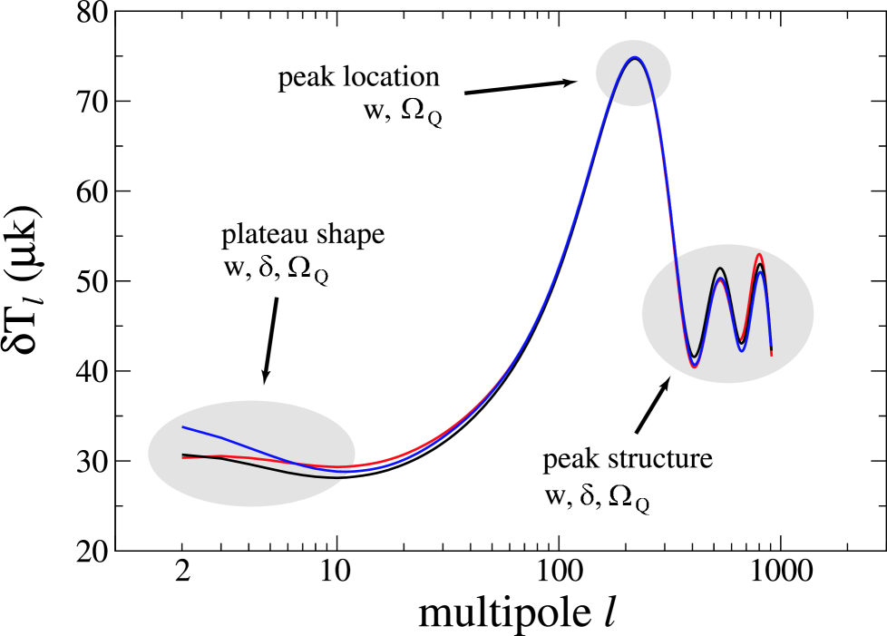
Figure 1: The pattern of CMB anisotropy can reveal information about the quintessence abundance ($\Omega_{Q}$), equation-of-state ($w$), and behavior of fluctuations ($\delta$). The three curves are examples of constant equation-of-state models which differ little by eye, but are distinguished by the data. The red ($w=-0.5$) and blue ($-1.2$) curves are both low-$\chi^{2}$ CMB-indistinguishable, but distinct with respect to SNe. The black curve ($-0.8$), although it is consistent with the SNe data and matches the location and height of the first acoustic peak determined by WMAP Page:2003fa , is rejected by the CMB at the $3\sigma$-level.

In this article we test the quintessence hypothesis, that a dynamical, time-evolving, negative pressure, inhomogeneous form of energy dominates the cosmic energy density and is responsible for the cosmic acceleration Ratra:1987rm ; Peebles:1987ek ; Wetterich:fm ; Wetterich:bg ; Coble:1996te ; Caldwell:1997ii ; Turner:1998ex . To be precise, we carry out an extensive analysis of the CMB anisotropy and mass fluctuation spectra for a wide range of quintessence models. These models are: (Q1) models with a constant equation-of-state, $w$, including $w<-1$; (Q2) models with a simply-parametrized, time-evolving $w$; (Q3) early quintessence models, with a non-negligible energy density during the recombination era; (Q4) trackers described by a scalar field evolving under an inverse-power law potential.

The suite of parameters describing the cosmological models are split into spacetime plus “matter sector” variables, $\theta_{M}$, and separate quintessence parameters, $\theta_{Q}$. The spacetime and “matter sector” of the quintessence models are specified by the parameter set $\theta_{M}=\{\Omega_{b}h^{2},\,\Omega_{cdm}h^{2},\,h,\,n_{s},\,A_{S},\,\tau_{r}\}$. In order, these are the baryon density, cold dark matter density, hubble parameter, scalar perturbation spectral index, scalar perturbation amplitude, and optical depth. In this investigation we restrict our attention to spatially-flat, cold dark matter models with a primordial spectrum of nearly scale-invariant density perturbations generated by inflation.

The quintessence parameters vary from model to model. For the simplest family of models, with a constant equation-of-state, we need only to specify $\theta_{Q}=\{w\}$. For models which feature more realistic time-evolution of the quintessence, which may include a non-negligible fraction of quintessence at early times, more parameters are required, e.g. $\theta_{Q}=\{w,\,dw/da,\,...\}$, to characterize the impact on the cosmology in general and the CMB in particular.

Our analysis method is as follows: (i) compute the CMB and fluctuation power spectra for a given cosmological model; (ii) compute the relative likelihood of the model with respect to the experimental data; (iii) assemble the likelihood function in parameter space to determine the range of viable quintessence models. For step (i) we use both a version of CMBfast CMBfast modified for quintessence, as well as the newly-available CMBEASY CMBEASY . For step (ii) we supplement the WMAP data with the complementary ACBAR ACBAR and CBI-MOSAIC data CBI_mosaic ; CBI_deep (using the same bins as Ref. Spergel:2003cb ; Verde:2003ey ), in addition to the current type 1a SNe data Schmidt:1998ys ; Riess:1998cb ; Garnavich:1998th ; Perlmutter:1998np . Certain other constraints, such as the HST Key Project measurement of $H_{0}$ Freedman:2000cf or the limit from Big Bang Nucleosynthesis on $\Omega_{b}h^{2}$ Burles:2000zk through the deuterium abundance measurement are satisfied as cross-checks. It is remarkable that such agreement can be found between such diverse phenomena. Our focus in the following investigation, however, is primarily on the CMB and SNe.

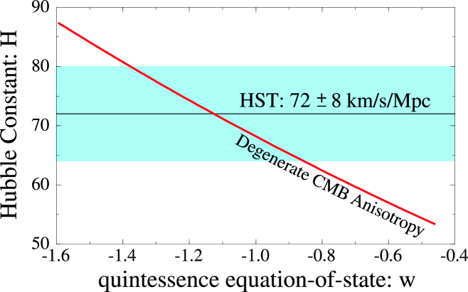
Figure 2: The one-parameter family of best-fit models, which exploit the geometric degeneracy of the CMB anisotropy pattern, is shown as the thick, red curve in the $w-h$ plane. We have explored models in a six-dimensional cylinder in the parameter space surrounding this “best-fit line.” The HST-Key Project $1\sigma$ measurement of the Hubble constant is shown by the shaded band.

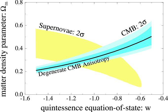
Figure 3: The constraints on constant equation-of-state models due to CMB (WMAP, ACBAR, CBI) and type 1a supernovae (Hi-Z, SCP) are shown. The starting point for our parameter-search, the family of CMB-degenerate models, is shown by the thick, black line.

Q1: We have analyzed the cosmological constraints on the simplest model of quintessence, characterized by a constant equation-of-state, $w$. We have used the equivalence between a scalar field $\varphi$ with potential $V(\varphi)$ and the equation-of-state $w$ in order to self-consistently evaluate the quintessence fluctuations. For the range $w<-1$ we employ a k essence model, keeping the sound speed (actually, this is $d\omega^{2}/dk^{2}$) fixed at $c_{s}^{2}=1$. Since this model introduces only one additional parameter beyond the basic set of spacetime plus matter sector variables, we adopt a simplistic grid-based search for viable models. The acceptance criteria for the Q1 models is based on a $\Delta\chi^{2}$-test. The results of our survey of Q1 models are shown in Figures 2, 3. We have exploited the degeneracy of the CMB anisotropy pattern among models with the same apparent angular size of the last scattering horizon Huey:1998se . Hence, there is a family of models with $\Omega_{b}h^{2}=0.023$, $\Omega_{cdm}h^{2}=0.126$, $n_{s}=0.97$, and characterized by pairs $\{w,\ h\}$ having (nearly) indistinguishable CMB anisotropy patterns. The pairs $\{w,\ h\}$ are shown in Figure 2, and all represent quintessence models with $\chi^{2}=1429$ for the WMAP temperature-temperature and temperature-polarization data — a one-parameter family of best-fit models. From this starting point, we explored over $6\times 10^{4}$ models distributed on a grid filling a 6-cylinder around the best-fit line, varying $\{\Omega_{b}h^{2},\,\Omega_{cdm}h^{2},\,h,\,n_{s},\,\tau_{r}\}$ at intervals in $w$. For each model we evaluate the likelihood relative to WMAP, as well as the complementary ACBAR and CBI-MOSAIC data. The $2\sigma$ boundary, based on a $\Delta\chi^{2}$ test for six degrees of freedom is shown in Figure 3. We have also evaluated the constraint in the $w-\Omega_{m}$ plane for the combined Hi-Z/SCP type 1a supernova data set, showing the $2\sigma$ region based on a $\Delta\chi^{2}$ test for two degrees of freedom. Our basic conclusion from the overlapping constraint regions is that there exist concordant models with $-1.25\lesssim w\lesssim-0.8$ and $0.25\lesssim\Omega_{m}\lesssim 0.4$. We have identified four sample models in Table 1 for further analysis.

model	$w$	$h$	$\sigma_{8}$
Q1.1	-0.82	0.630	0.84
Q1.2	-1.00	0.682	0.89
Q1.3	-1.18	0.737	0.96
Q1.4	-1.25	0.759	0.97

Table 1: Sample best-fit models with a constant equation-of-state (Q1). All models have $\Omega_{b}h^{2}=0.023$, $\Omega_{cdm}h^{2}=0.126$, $n_{s}=0.97$, and $\tau_{r}=0.11$.

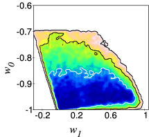
(a) Q2: monotonic evolution $w(a)$

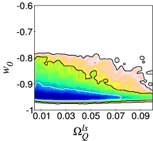
(b) Q3: leaping kinetic quintessence

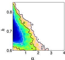
(c) Q4: inverse-power law

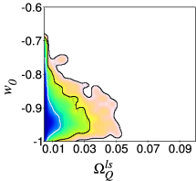
(d) Q2: monotonic evolution $w(a)$

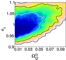
(e) Q3: leaping kinetic quintessence

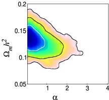
(f) Q4: inverse-power law

Figure 4: The results of our MCMC search of the multi-dimensional parameter search, for models Q2-4, are illustrated in the figures above. In all cases, we have marginalized over the suppressed parameters. The solid lines indicate the $1,\,2,\,3\sigma$ contours based on comparison with the CMB (WMAP, ACBAR, CBI) and type 1a supernovae (Hi-Z, SCP).

Our search of the parameter space for the remaining models is based on a Bayesian approach, using a Monte-Carlo Markov-Chain (MCMC) search algorithm to identify the best cosmological models. The end product is a realization of the posterior probability distribution function on the parameter space Christensen:2001gj . Our approach is similar to the procedure described in Verde:2003ey , whereby the MCMC makes a “smart” walk through the parameter space, accepting or rejecting sampled points based on a running criteria. For each of Q2-4, after some experimentation we found it practical to use four independent chains in order to monitor convergence and mixing according to the criteria of Ref. Gelman::1992 . Each such chain explored $\sim 3\times 10^{4}$ models. We found it advantageous to use a dynamical stepsize factor $r\in[0.1,10]$. In each step, all parameters are varied according to a Gaussian with width $r\sigma_{i}$, where $\sigma_{i}$ is an initial stepsize for the random walk in the direction of the $i$-th parameter. The stepsize factor $r$ is adjusted such that the chain neither rejects nor accepts too frequently. Certain parameters, such as $w_{0}$ and $\Omega_{Q}^{ls}$ in the early quintessence models, have physical boundaries and it is therefore important that our MCMC does not lead to a bias in the sampled distribution close to the boundaries. As the likelihood in the MCMC approach is given by the frequency with which the chain passes through a given region of parameter space, we would be in danger of depleting the region close to the boundary if we were to simply discard any steps which cross the boundary. That is, the likelihood in the parameter region close to the boundary would be artificially suppressed. If such a (virtual) jump in a parameter direction $i$ occurs, we use the following strategy. We try making a gaussian-weighted step but only towards the boundary. If this fails after ten attempts, then we start over again by making a gaussian step in any direction. By trying ten times, however, it is very likely that we do make the step successfully, if we are at least one $\sigma_{i}$ away from the boundary. If, however, we are very close to the boundary already and our step would have carried us deep into the unphysical region, then it is sensible to make the step away from the current point, for the chain didn’t intend to stay close to the boundary anyhow. To give us confidence in the reliability of this algorithm, we have checked by synthetic distributions that this strategy is very well suited for sampling the likelihood, even in cases where a physical boundary cuts off the parameter space.

Q2: We have examined quintessence models with an equation-of-state that evolves monotonically with the scale factor, as $w(a)=w_{0}+(1-a)w_{1}$. For this case, the parameters are simply $\theta_{Q}=\{w_{0},\,w_{1}\}$. This parametrization has been shown to be versatile in describing the late-time quintessence evolution for a wide class of scalar field models Linder:2002et . Based on the degeneracy of models found for Q1, we expect to find a two-dimensional family of equivalent best-fit models with the same apparent angular size of the last scattering horizon, occupying a plane in the $\{w_{0},\,w_{1},\,h\}$ space. There are three ways in which this plane is pared down: Firstly we confine $w\geq-1$ at all times. Secondly, the transition from $w_{0}$ to $w_{0}+w_{1}$ takes place at low redshift, $z\lesssim 1$, so that high redshift supernovae restrict $w_{0},\ w_{1}$ for these models. Thirdly, this parametrization allows for models in which the dark energy is non-negligible at early times, which influences the small-scale fluctuation spectrum. The first two considerations yield $w_{0}<-0.75$ at the $2\sigma$ level, marginalizing over the suppressed five dimensional parameter space, as illustrated in Figure 4(a). There, the shapes of the contours indicate that current data can only distinguish between fast ($dw/da\gtrsim 0.5$) and slow evolution of $w(a)$, and offer only a weak bound on $w_{1}$. However, in terms of $\Omega_{Q}^{ls}$, our third consideration gives a tight upper bound on the quintessence density during recombination. As shown in Figure 4(d), $\Omega_{Q}^{ls}<0.03$ at the $2\sigma$ level. Three target models, with significantly different equation-of-state evolution $dw/da$, are given in Table 2 for future investigations.

model	$w_{0}$	$w_{1}$	$h$	$\Omega_{Q}^{ls}$	$\sigma_{8}$
Q2.1	-0.93	0.43	0.66	$4\times 10^{-6}$	0.77
Q2.2	-0.99	0.68	0.64	$1\times 10^{-4}$	0.78
Q2.3	-0.92	0.62	0.62	$1\times 10^{-4}$	0.73

Table 2: Sample best-fit models with a monotonically-evolving equation-of-state (Q2). Although a range of parameters give equivalently good fits to the observational data, we have selected this sample with $\{\Omega_{b}h^{2},\ \Omega_{cdm}h^{2},\ n_{s},\ \tau_{r}\}$ = $\{0.023,\ 0.11,\ 0.98,\ 0.16\}$ (Q2.1), $\{0.023,\ 0.11,\ 0.98,\ 0.15\}$ (Q2.2), $\{0.023,\ 0.12,\ 0.98,\ 0.08\}$ (Q2.3), Entries for $\Omega_{Q}^{ls}$ and $\sigma_{8}$ are the resulting values based on the other parameters.

Q3: We have examined models of leaping kinetic quintessence, a scalar field evolving under an exponential potential with a non-canonical kinetic term that undergoes a sharp transition at late times, leading to the current accelerated expansion Hebecker:2000zb . At early times the field closely tracks the cosmological background with $w=0$ during matter domination, appearing as early quintessence Caldwell:2003vp before undergoing a steep transition towards a strongly negative equation-of-state by the present day. The steepness of the transition in $w$ for a leaping kinetic model is directly connected to the equation-of-state $w_{0}$ today. Such models can therefore be characterized by the parameters $\theta_{Q}=\{\Omega_{Q}^{ls},w_{0}\}$, where $\Omega_{Q}^{ls}$ is the quintessence density during recombination. (A more general parameterization, allowing for independent $w_{0}$ and steepness of transition can be found in Corasaniti:2002vg .) Since $\Omega_{Q}^{ls}$ is not tied as closely to the expansion rate sampled by the supernovae, compared to case Q2, the result is the weaker constraint $\Omega_{Q}^{ls}\lesssim 0.1$, as shown in Figure 4(b). Although the limit of a cosmological constant can be approached in this model, the presence of early quintessence will then require a sharp transition in the equation-of-state in order to reach $w\to-1$. In addition to the fact that such models lose the early tracking behavior and instead require some degree of fine-tuning, there is the practical consideration that the sharp transition leads to some numerical instability in our code. To avoid this problem, we restrict $w>-0.97$ as can be seen in Figure 4(b). We believe that we have succeeded at implementing an MCMC algorithm that does not artificially distort the probability distribution near the parameter-space boundaries, based on our experimentation with synthetic distributions with boundaries. Next, because early quintessence suppresses the growth of fluctuations on small scales compared to large scales, we find that comparable fluctuation spectra can be achieved by making a trade-off between $n_{s}$ and $\Omega_{Q}^{ls}$. As shown in Figure 4(e), slight suppression of small-scale power can be accomplished either by a tilt towards the red, $n_{s}<1$, or a rise in $\Omega_{Q}^{ls}$. Since the effect of early quintessence on the small-scale fluctuation power spectrum closely mimics a running spectral index, we have not introduced ${\rm d}n_{s}/{\rm d}\ln k$ as an additional parameter, which would be highly degenerate with $\Omega_{Q}^{ls}$ Caldwell:2003vp . We expect that improved measurements of the second and third acoustic peaks will tighten the constraint on $\Omega_{Q}^{ls}$ and sharpen the degeneracy in the $n_{s}-\Omega_{Q}^{ls}$ plane. Target models, with significantly different values of early quintessence abundance, are given in Table 3.

model	$w_{0}$	$\Omega_{Q}^{ls}$	$h$	$A$	$\bar{w}_{ls}$	$\sigma_{8}$
Q3.1	-0.94	0.006	0.69	0.0026	-0.27	0.89
Q3.2	-0.91	0.024	0.70	-0.0028	-0.21	0.81
Q3.3	-0.93	0.043	0.71	-0.0070	-0.19	0.85

Table 3: Sample best-fit leaping-kinetic quintessence models (Q3). The parameters A is an equivalent description of $\Omega_{Q}^{ls}$, which along with the averaged $w$ at last scattering, $\bar{w}_{ls}$, can be used more easily with equations 2-4 of Ref. Caldwell:2003vp to generate the time-evolution of these models. The non-quintessence parameters are $\{\Omega_{b}h^{2},\ \Omega_{cdm}h^{2},\ n_{s},\ \tau_{r}\}$ = $\{0.022,\ 0.112,\ 0.96,\ 0.12\}$ (Q3.1), $\{0.023,\ 0.116,\ 1.0,\ 0.16\}$ (Q3.2), $\{0.024,\ 0.119,\ 1.04,\ 0.26\}$ (Q3.3).

Q4: Finally, we have examined tracker models of quintessence. Inverse-power law (IPL) models are the archetype quintessence models with tracking property and acceleration Ratra:1987rm ; Zlatev:1998tr ; Steinhardt:nw . The potential is given by $V\propto\varphi^{-\alpha}$, where the constant of proportionality is determined by $\Omega_{Q}$. In certain supersymmetric QCD realizations of the IPL Masiero:1999sq , $\alpha$ is related to the numbers of color and flavors, and can take on a continuous range of values $\alpha>0$. For $\alpha\to 0$, however, inverse-power law models behave more and more like a cosmological constant. Using earlier data, $\alpha$ has been constrained to $\alpha<1.4$ Balbi:2000kj ; Baccigalupi:2001aa , although $h=0.65$ has been fixed in those analyses. Keeping $h$ free, a more conservative value of $\alpha<2$ Doran:2001ty was inferred. From our analysis, we see that the $2\sigma$ bound has not changed dramatically. The $2\sigma$-bound with $\alpha\lesssim 1-2$ is consistent with values of $h$ within the range determined by the HST, as seen in Figure 4(c). In Figure 4(f) we plot the likelihood contours in the $\Omega_{m}h^{2}-\alpha$ plane: our results agree with the best fit at $\Omega_{m}h^{2}=0.149$ for $\alpha=0$ or $w=-1$, but show a tolerance for a wider range for $0\leq\alpha\leq 2$. That is, the additional degree of freedom in $\alpha$ means that the matter density for the IPL model is not as well-determined from the peak position Page:2003fa as compared to the $\Lambda$ model. However, to maintain the peak at $\ell=220$, we observe that $\Omega_{m}h^{2}$ decreases slightly as $\alpha$ increases. We might have inferred the results for the IPL based on the constant equation-of-state models: pairs of $\{\alpha,\ h\}$ can equivalently determine a family of models with degenerate CMB anisotropy patterns, since the differences in the late-ISW for this model compared to Q1 make only a small contribution to the overall $\chi^{2}$. Furthermore, since IPL quintessence can be modeled by the appropriate choice of the Q2 parameters, then improved sensitivity to $dw/da$ is required to tighten the constraints here. While $\alpha$ is tightly constrained, our take-away is that IPL models with $0.25\lesssim\Omega_{m}\lesssim 0.4$ remain viable. Target models are given in Table 4.

model	$\alpha$	$h$	$\sigma_{8}$
Q4.1	0.1	0.68	0.90
Q4.2	0.2	0.68	0.85
Q4.3	0.8	0.68	0.82

Table 4: Sample best-fit IPL quintessence models (Q4). The non-quintessence parameters are $\{\Omega_{b}h^{2},\ \Omega_{cdm}h^{2},\ n_{s},\ \tau_{r}\}$ = $\{0.023,\ 0.122,\ 0.97,\ 0.13\}$ (Q4.1), $\{0.023,\ 0.116,\ 0.97,\ 0.14\}$ (Q4.2), $\{0.024,\ 0.102,\ 1.0,\ 0.23\}$ (Q4.3).

This work provides a capsule summary of the viable quintessence dark energy models, based on two of the tightest constraint methods, using the CMB and SNe. Our study advances beyond past investigations Baccigalupi:2001aa ; Brax:2000yb ; Corasaniti:2001mf ; Bean:2001xy ; Hannestad:2002ur ; Bassett:2002fe ; Jimenez:2003iv ; Barreiro:2003ua by treating a wide class of quintessence models with the powerful weight of the WMAP data. We have considered four classes of models which cover the most basic quintessence scenarios, including a versatile parametrization, as well as the best motivated and most realistic scenarios based on our current understanding of particle physics. Absent from our survey are k essence models, and dark energy models with a coupling to other matter fields or gravity. In the former case, since the sound speed of fluctuations varies with time in these models, however, we can make a simple distinction with quintessence models with an underlying scalar field, wherein the propagation speed is equal to the speed of light. (See Refs. Erickson:2001bq ; DeDeo:2003te for analysis of these models with respect to CMB anisotropy.) For the latter case we refer to Ref. Amendola:2003eq for specific coupled models. We also note that the mass fluctuation power spectrum is an important cosmological constraint which we have omitted at this stage, primarily because it constrains energy density rather than pressure (although there are exceptions), a chief feature distinguishing dark energy from dark matter. (The constraint curves obtained in Ref. Schuecker:2002yj , e.g. Figure 3, are consistent with, but do not decisively pare down the parameter regions of our current results.) Furthermore, the analysis of mass power spectrum observations will have to take into account possible influences of a time-dependent $w$ and early quintessence, which we put off for later investigation. Overall, we have simulated in detail more than 400,000 individual cosmological models. The stored spectra and parameter-space likelihood functions will be used to evaluate additional constraints that can offer clues to the behavior of the dark energy. The set of thirteen target models, listed in Tables 1-4, which includes a revised concordance $\Lambda$ model Wang:1999fa , should be of use by researchers to further test the quintessence hypothesis.

Acknowledgments  This work was supported by NSF grant PHY-0099543 at Dartmouth. We thank Pier Stefano Corasaniti for useful conversations, and Dartmouth colleagues Barrett Rogers and Brian Chaboyer for use of computing resources.

References

- (1) C. L. Bennett et al., Astrophys. J. 583, 1 (2003) [arXiv:astro-ph/0301158].
- (2) C. L. Bennett et al., arXiv:astro-ph/0302207.
- (3) G. Hinshaw et al., arXiv:astro-ph/0302217.
- (4) A. Kogut et al., arXiv:astro-ph/0302213.
- (5) L. Page et al., arXiv:astro-ph/0302220.
- (6) D. N. Spergel et al., arXiv:astro-ph/0302209.
- (7) L. Verde et al., arXiv:astro-ph/0302218.
- (8) B. Ratra and P. J. Peebles, Phys. Rev. D 37, 3406 (1988).
- (9) P. J. Peebles and B. Ratra, Astrophys. J. 325, L17 (1988).
- (10) C. Wetterich, Nucl. Phys. B 302, 668 (1988).
- (11) C. Wetterich, Astron. Astrophys. 301, 321 (1995).
- (12) K. Coble, S. Dodelson and J. A. Frieman, Phys. Rev. D 55, 1851 (1997).
- (13) R. R. Caldwell, R. Dave and P. J. Steinhardt, Phys. Rev. Lett. 80, 1582 (1998).
- (14) M. S. Turner and M. J. White, Phys. Rev. D 56, 4439 (1997).
- (15) U. Seljak and M. Zaldarriaga, Astrophys. J. 469, 437 (1996).
- (16) Doran, M., “CMBEASY :: an Object Oriented Code for the Cosmic Microwave Background,” [arXiv: astro-ph/0302138]; software available at www.cmbeasy.org.
- (17) C. L. Kuo et al., arXiv:astro-ph/0212289.
- (18) T. J. Pearson et al., arXiv:astro-ph/0205388.
- (19) B. S. Mason et al., arXiv:astro-ph/0205384.
- (20) B. P. Schmidt et al., Astrophys. J. 507, 46 (1998).
- (21) A. G. Riess et al., Astron. J. 116, 1009 (1998).
- (22) P. M. Garnavich et al., Astrophys. J. 509, 74 (1998).
- (23) S. Perlmutter et al., Astrophys. J. 517, 565 (1999).
- (24) W. L. Freedman et al., Astrophys. J. 553, 47 (2001).
- (25) S. Burles, K. M. Nollett and M. S. Turner, Astrophys. J. 552, L1 (2001).
- (26) G. Huey, L. M. Wang, R. Dave, R. R. Caldwell and P. J. Steinhardt, Phys. Rev. D 59, 063005 (1999).
- (27) N. Christensen, R. Meyer, L. Knox and B. Luey, arXiv:astro-ph/0103134.
- (28) A. Gelman and D. Rubin, Statistical Science, 7, 457 (1992).
- (29) E. V. Linder, Phys. Rev. Lett. 90, 091301 (2003).
- (30) A. Hebecker and C. Wetterich, Phys. Lett. B 497, 281 (2001).
- (31) R. R. Caldwell, M. Doran, C. M. Mueller, G. Schaefer and C. Wetterich, [arXiv:astro-ph/0302505].
- (32) P. S. Corasaniti and E. J. Copeland, Phys. Rev. D 67, 063521 (2003).
- (33) I. Zlatev, L. M. Wang and P. J. Steinhardt, Phys. Rev. Lett. 82, 896 (1999).
- (34) P. J. Steinhardt, L. M. Wang and I. Zlatev, Phys. Rev. D 59, 123504 (1999).
- (35) A. Masiero, M. Pietroni and F. Rosati, Phys. Rev. D 61, 023504 (2000).
- (36) A. Balbi, C. Baccigalupi, S. Matarrese, F. Perrotta and N. Vittorio, Astrophys. J. 547, L89 (2001).
- (37) C. Baccigalupi, A. Balbi, S. Matarrese, F. Perrotta and N. Vittorio, Phys. Rev. D 65, 063520 (2002).
- (38) M. Doran, M. Lilley and C. Wetterich, Phys. Lett. B 528, 175 (2002).
- (39) P. Brax, J. Martin and A. Riazuelo, Phys. Rev. D 62, 103505 (2000).
- (40) P. S. Corasaniti and E. J. Copeland, Phys. Rev. D 65, 043004 (2002).
- (41) R. Bean and A. Melchiorri, Phys. Rev. D 65, 041302 (2002).
- (42) S. Hannestad and E. Mortsell, Phys. Rev. D 66, 063508 (2002).
- (43) B. A. Bassett, M. Kunz, D. Parkinson and C. Ungarelli, arXiv:astro-ph/0211303.
- (44) R. Jimenez, L. Verde, T. Treu and D. Stern, arXiv:astro-ph/0302560.
- (45) T. Barreiro, M. C. Bento, N. M. Santos and A. A. Sen, arXiv:astro-ph/0303298.
- (46) J. K. Erickson, R. R. Caldwell, P. J. Steinhardt, C. Armendariz-Picon and V. Mukhanov, Phys. Rev. Lett. 88, 121301 (2002).
- (47) S. DeDeo, R. R. Caldwell and P. J. Steinhardt, arXiv:astro-ph/0301284.
- (48) L. Amendola and C. Quercellini, arXiv:astro-ph/0303228.
- (49) P. Schuecker, R. R. Caldwell, H. Bohringer, C. A. Collins and L. Guzzo, Type-Ia Supernovae,” arXiv:astro-ph/0211480.
- (50) L. M. Wang, R. R. Caldwell, J. P. Ostriker and P. J. Steinhardt, Astrophys. J. 530, 17 (2000).